Computer Methods for Ordinary Differential Equations and Differential Algebraic Equations
Bạn đang xem bản rút gọn của tài liệu. Xem và tải ngay bản đầy đủ của tài liệu tại đây (3.09 MB, 330 trang )
Computer Methods for Ordinary Di erential
Equations and Di erential-Algebraic
Equations
Uri M. Ascher and Linda R. Petzold
December 2, 1997
Preface
This book has been developed from course notes that we wrote, having
repeatedly taught courses on the numerical solution of ordinary di erential
equations (ODEs) and related problems. We have taught such courses at a
senior undergraduate level as well as at the level of a rst graduate course on
numerical methods for di erential equations. The audience typically consists
of students from Mathematics, Computer Science and a variety of disciplines
in engineering and sciences such as Mechanical, Electrical and Chemical Engineering, Physics, Earth Sciences, etc.
The material that this book covers can be viewed as a rst course on the
numerical solution of di erential equations. It is designed for people who
want to gain a practical knowledge of the techniques used today. The course
aims to achieve a thorough understanding of the issues and methods involved
and of the reasons for the successes and failures of existing software. On one
hand, we avoid an extensive, thorough, theorem-proof type exposition: we
try to get to current methods, issues and software as quickly as possible.
On the other hand, this is not a quick recipe book, as we feel that a deeper
understanding than can usually be gained by a recipe course is required to
enable the student or the researcher to use their knowledge to design their
own solution approach for any nonstandard problems they may encounter in
future work. The book covers initial-value and boundary-value problems, as
well as di erential-algebraic equations (DAEs). In a one-semester course we
have been typically covering over 75% of the material it contains.
We wrote this book partially as a result of frustration at not being able
to assign a textbook adequate for the material that we have found ourselves
covering. There is certainly excellent, in-depth literature around. In fact, we
are making repeated references to exhaustive texts which, combined, cover
almost all the material in this book. Those books contain the proofs and
references which we omit. They span thousands of pages, though, and the
time commitment required to study them in adequate depth may be more
than many students and researchers can a ord to invest. We have tried to
stay below a 350-page limit and to address all three ODE-related areas menii
iii
tioned above. A signi cant amount of additional material is covered in the
Exercises. Other additional important topics are referred to in brief sections
of Notes and References. Software is an important and well-developed part
of this subject. We have attempted to cover the most fundamental software
issues in the text. Much of the excellent and publicly-available software is
described in the Software sections at the end of the relevant chapters, and
available codes are cross-referenced in the index. Review material is highlighted and presented in the text when needed, and it is also cross-referenced
in the index.
Traditionally, numerical ODE texts have spent a great deal of time developing families of higher order methods, e.g. Runge-Kutta and linear multistep methods, applied rst to nonsti problems and then to sti problems.
Initial value problems and boundary value problems have been treated in
separate texts, although there is much in common. There have been fundamental di erences in approach, notation, and even in basic de nitions,
between ODE initial value problems, ODE boundary value problems, and
partial di erential equations (PDEs).
We have chosen instead to focus on the classes of problems to be solved,
mentioning wherever possible applications which can lend insight into the
requirements and the potential sources of di culty for numerical solution.
We begin by outlining the relevant mathematical properties of each problem
class, then carefully develop the lower-order numerical methods and fundamental concepts for the numerical analysis. Next we introduce the appropriate families of higher-order methods, and nally we describe in some detail
how these methods are implemented in modern adaptive software. An important feature of this book is that it gives an integrated treatment of ODE
initial value problems, ODE boundary value problems, and DAEs, emphasizing not only the di erences between these types of problems but also the
fundamental concepts, numerical methods and analysis which they have in
common. This approach is also closer to the typical presentation for PDEs,
leading, we hope, to a more natural introduction to that important subject.
Knowledge of signi cant portions of the material in this book is essential
for the rapidly emerging eld of numerical dynamical systems. These are numerical methods employed in the study of the long term, qualitative behavior
of various nonlinear ODE systems. We have emphasized and developed in
this work relevant problems, approaches and solutions. But we avoided developing further methods which require deeper, or more speci c, knowledge
of dynamical systems, which we did not want to assume as a prerequisite.
The plan of the book is as follows. Chapter 1 is an introduction to the
di erent types of mathematical models which are addressed in the book.
We use simple examples to introduce and illustrate initial- and boundaryvalue problems for ODEs and DAEs. We then introduce some important
applications where such problems arise in practice.
iv
Each of the three parts of the book which follow starts with a chapter
which summarizes essential theoretical, or analytical issues (i.e. before applying any numerical method). This is followed by chapters which develop
and analyze numerical techniques. For initial value ODEs, which comprise
roughly half this book, Chapter 2 summarizes the theory most relevant for
computer methods, Chapter 3 introduces all the basic concepts and simple
methods (relevant also for boundary value problems and for DAEs), Chapter
4 is devoted to one-step (Runge-Kutta) methods and Chapter 5 discusses
multistep methods.
Chapters 6-8 are devoted to boundary value problems for ODEs. Chapter
6 discusses the theory which is essential to understand and to make e ective
use of the numerical methods for these problems. Chapter 7 brie y considers shooting-type methods and Chapter 8 is devoted to nite di erence
approximations and related techniques.
The remaining two chapters consider DAEs. This subject has been researched and solidi ed only very recently (in the past 15 years). Chapter 9
is concerned with background material and theory. It is much longer than
Chapters 2 and 6 because understanding the relationship between ODEs and
DAEs, and the questions regarding reformulation of DAEs, is essential and
already suggests a lot regarding computer approaches. Chapter 10 discusses
numerical methods for DAEs.
Various courses can be taught using this book. A 10-week course can be
based on the rst 5 chapters, with an addition from either one of the remaining two parts. In a 13-week course (or shorter in a more advanced graduate
class) it is possible to cover comfortably Chapters 1-5 and either Chapters 6-8
or Chapters 9-10, with a more super cial coverage of the remaining material.
The exercises vary in scope and level of di culty. We have provided some
hints, or at least warnings, for those exercises that we (or our students) have
found more demanding.
Many people helped us with the tasks of shaping up, correcting, ltering
and re ning the material in this book. First and foremost there are our
students in the various classes we taught on this subject. They made us
acutely aware of the di erence between writing with the desire to explain
and writing with the desire to impress. We note, in particular, G. Lakatos,
D. Aruliah, P. Ziegler, H. Chin, R. Spiteri, P. Lin, P. Castillo, E. Johnson,
D. Clancey and D. Rasmussen. We have bene ted particularly from our
earlier collaborations on other, related books with K. Brenan, S. Campbell,
R. Mattheij and R. Russell. Colleagues who have o ered much insight, advice
and criticism include E. Biscaia, G. Bock, C. W. Gear, W. Hayes, C. Lubich,
V. Murata, D. Pai, J. B. Rosen, L. Shampine and A. Stuart. Larry Shampine,
in particular, did an incredibly extensive refereeing job and o ered many
comments which have helped us to signi cantly improve this text. We have
v
PREFACE
also bene ted from comments of numerous anonymous referees.
December 2, 1997
U. M. Ascher
L. R. Petzold
vi
PREFACE
Contents
1 Ordinary Di erential Equations
1.1
1.2
1.3
1.4
1.5
1.6
Initial Value Problems . . . . . .
Boundary Value Problems . . . .
Di erential-Algebraic Equations .
Families of Application Problems
Dynamical Systems . . . . . . . .
Notation . . . . . . . . . . . . . .
.
.
.
.
.
.
.
.
.
.
.
.
.
.
.
.
.
.
2 On Problem Stability
2.1
2.2
2.3
2.4
2.5
2.6
2.7
Test Equation and General De nitions
Linear, Constant Coe cient Systems .
Linear, Variable Coe cient Systems . .
Nonlinear Problems . . . . . . . . . . .
Hamiltonian Systems . . . . . . . . . .
Notes and References . . . . . . . . . .
Exercises . . . . . . . . . . . . . . . . .
3 Basic Methods, Basic Concepts
3.1
3.2
3.3
3.4
3.5
3.6
3.7
3.8
.
.
.
.
.
.
.
.
.
.
.
.
.
.
.
.
.
.
.
.
.
.
.
.
.
.
.
.
.
.
.
.
.
.
.
.
.
.
.
.
.
.
.
.
.
.
.
.
.
.
.
.
.
.
.
.
.
.
.
.
.
.
.
.
.
.
.
.
.
.
.
.
.
.
.
.
.
.
.
.
.
.
.
.
.
.
.
.
.
.
.
A Simple Method: Forward Euler . . . . . . . . . .
Convergence, Accuracy, Consistency and 0-Stability
Absolute Stability . . . . . . . . . . . . . . . . . . .
Sti ness: Backward Euler . . . . . . . . . . . . . .
A-Stability, Sti Decay . . . . . . . . . . . . . . . .
Symmetry: Trapezoidal Method . . . . . . . . . . .
Rough Problems . . . . . . . . . . . . . . . . . . .
Software, Notes and References . . . . . . . . . . .
3.8.1 Notes . . . . . . . . . . . . . . . . . . . . .
3.8.2 Software . . . . . . . . . . . . . . . . . . . .
3.9 Exercises . . . . . . . . . . . . . . . . . . . . . . . .
4 One Step Methods
.
.
.
.
.
.
.
.
.
.
.
.
.
.
.
.
.
.
.
.
.
.
.
.
.
.
.
.
.
.
.
.
.
.
.
.
.
.
.
.
.
.
.
.
.
.
.
.
.
.
.
.
.
.
.
.
.
.
.
.
.
.
.
.
.
.
.
.
.
.
.
.
.
.
.
.
.
.
.
.
.
.
.
.
.
.
.
.
.
.
.
.
.
.
.
.
.
.
.
.
.
.
.
.
.
.
.
.
.
.
.
.
.
.
.
.
.
.
.
.
.
.
.
.
.
.
.
.
.
.
.
.
.
.
.
.
.
.
.
.
.
.
.
.
1
3
8
9
11
15
16
19
21
22
26
28
29
31
31
35
35
38
42
47
56
58
61
64
64
65
67
73
4.1 The First Runge-Kutta Methods . . . . . . . . . . . . . . . . 75
4.2 General Formulation of Runge-Kutta Methods . . . . . . . . . 81
vii
viii
CONTENTS
4.3
4.4
4.5
4.6
4.7
Convergence, 0-Stability and Order for Runge-Kutta Methods 83
Regions of Absolute Stability for Explicit Runge-Kutta Methods 89
Error Estimation and Control . . . . . . . . . . . . . . . . . . 91
Sensitivity to Data Perturbations . . . . . . . . . . . . . . . . 96
Implicit Runge-Kutta and Collocation Methods . . . . . . . . 101
4.7.1 Implicit Runge-Kutta Methods Based on Collocation . 102
4.7.2 Implementation and Diagonally Implicit Methods . . . 105
4.7.3 Order Reduction . . . . . . . . . . . . . . . . . . . . . 108
4.7.4 More on Implementation and SIRK Methods . . . . . . 109
4.8 Software, Notes and References . . . . . . . . . . . . . . . . . 110
4.8.1 Notes . . . . . . . . . . . . . . . . . . . . . . . . . . . 110
4.8.2 Software . . . . . . . . . . . . . . . . . . . . . . . . . . 112
4.9 Exercises . . . . . . . . . . . . . . . . . . . . . . . . . . . . . . 113
5 Linear Multistep Methods
125
6 More BVP Theory and Applications
163
5.1 The Most Popular Methods . . . . . . . . . . . . . . . . . . . 127
5.1.1 Adams Methods . . . . . . . . . . . . . . . . . . . . . . 128
5.1.2 Backward Di erentiation Formulae . . . . . . . . . . . 131
5.1.3 Initial Values for Multistep Methods . . . . . . . . . . 132
5.2 Order, 0-Stability and Convergence . . . . . . . . . . . . . . . 134
5.2.1 Order . . . . . . . . . . . . . . . . . . . . . . . . . . . 134
5.2.2 Stability: Di erence Equations and the Root Condition 137
5.2.3 0-Stability and Convergence . . . . . . . . . . . . . . . 139
5.3 Absolute Stability . . . . . . . . . . . . . . . . . . . . . . . . . 143
5.4 Implementation of Implicit Linear Multistep Methods . . . . . 146
5.4.1 Functional Iteration . . . . . . . . . . . . . . . . . . . . 146
5.4.2 Predictor-Corrector Methods . . . . . . . . . . . . . . . 146
5.4.3 Modi ed Newton Iteration . . . . . . . . . . . . . . . . 148
5.5 Designing Multistep General-Purpose Software . . . . . . . . . 149
5.5.1 Variable Step-Size Formulae . . . . . . . . . . . . . . . 150
5.5.2 Estimating and Controlling the Local Error . . . . . . 152
5.5.3 Approximating the Solution at O -Step Points . . . . . 155
5.6 Software, Notes and References . . . . . . . . . . . . . . . . . 155
5.6.1 Notes . . . . . . . . . . . . . . . . . . . . . . . . . . . 155
5.6.2 Software . . . . . . . . . . . . . . . . . . . . . . . . . . 156
5.7 Exercises . . . . . . . . . . . . . . . . . . . . . . . . . . . . . . 157
6.1
6.2
6.3
6.4
6.5
Linear Boundary Value Problems and Green's Function
Stability of Boundary Value Problems . . . . . . . . . .
BVP Sti ness . . . . . . . . . . . . . . . . . . . . . . .
Some Reformulation Tricks . . . . . . . . . . . . . . . .
Notes and References . . . . . . . . . . . . . . . . . . .
.
.
.
.
.
.
.
.
.
.
.
.
.
.
.
. 166
. 168
. 171
. 172
. 174
CONTENTS
ix
6.6 Exercises . . . . . . . . . . . . . . . . . . . . . . . . . . . . . . 175
7 Shooting
7.1 Shooting: a Simple Method and its Limitations
7.1.1 Di culties . . . . . . . . . . . . . . . . .
7.2 Multiple Shooting . . . . . . . . . . . . . . . . .
7.3 Software, Notes and References . . . . . . . . .
7.3.1 Notes . . . . . . . . . . . . . . . . . . .
7.3.2 Software . . . . . . . . . . . . . . . . . .
7.4 Exercises . . . . . . . . . . . . . . . . . . . . . .
8 Finite Di erence Methods for BVPs
.
.
.
.
.
.
.
.
.
.
.
.
.
.
.
.
.
.
.
.
.
.
.
.
.
.
.
.
8.1 Midpoint and Trapezoidal Methods . . . . . . . . . . .
8.1.1 Solving Nonlinear Problems: Quasilinearization
8.1.2 Consistency, 0-stability and Convergence . . . .
8.2 Solving the Linear Equations . . . . . . . . . . . . . . .
8.3 Higher Order Methods . . . . . . . . . . . . . . . . . .
8.3.1 Collocation . . . . . . . . . . . . . . . . . . . .
8.3.2 Acceleration Techniques . . . . . . . . . . . . .
8.4 More on Solving Nonlinear Problems . . . . . . . . . .
8.4.1 Damped Newton . . . . . . . . . . . . . . . . .
8.4.2 Shooting for Initial Guesses . . . . . . . . . . .
8.4.3 Continuation . . . . . . . . . . . . . . . . . . .
8.5 Error Estimation and Mesh Selection . . . . . . . . . .
8.6 Very Sti Problems . . . . . . . . . . . . . . . . . . . .
8.7 Decoupling . . . . . . . . . . . . . . . . . . . . . . . .
8.8 Software, Notes and References . . . . . . . . . . . . .
8.8.1 Notes . . . . . . . . . . . . . . . . . . . . . . .
8.8.2 Software . . . . . . . . . . . . . . . . . . . . . .
8.9 Exercises . . . . . . . . . . . . . . . . . . . . . . . . . .
9 More on Di erential-Algebraic Equations
.
.
.
.
.
.
.
.
.
.
.
.
.
.
.
.
.
.
.
.
.
.
.
.
.
9.1 Index and Mathematical Structure . . . . . . . . . . . .
9.1.1 Special DAE Forms . . . . . . . . . . . . . . . . .
9.1.2 DAE Stability . . . . . . . . . . . . . . . . . . . .
9.2 Index Reduction and Stabilization: ODE with Invariant .
9.2.1 Reformulation of Higher-Index DAEs . . . . . . .
9.2.2 ODEs with Invariants . . . . . . . . . . . . . . .
9.2.3 State Space Formulation . . . . . . . . . . . . . .
9.3 Modeling with DAEs . . . . . . . . . . . . . . . . . . . .
9.4 Notes and References . . . . . . . . . . . . . . . . . . . .
9.5 Exercises . . . . . . . . . . . . . . . . . . . . . . . . . . .
.
.
.
.
.
.
.
.
.
.
.
.
.
.
.
.
.
.
.
.
.
.
.
.
.
.
.
.
.
.
.
.
.
.
.
.
.
.
.
.
.
.
.
.
.
.
.
.
.
.
.
.
.
.
.
.
.
.
.
.
.
.
.
.
.
.
.
.
.
.
177
. 177
. 180
. 183
. 186
. 186
. 187
. 187
193
. 194
. 197
. 201
. 204
. 206
. 206
. 208
. 210
. 210
. 211
. 211
. 213
. 215
. 220
. 222
. 222
. 223
. 223
231
. 232
. 238
. 245
. 247
. 248
. 250
. 253
. 254
. 256
. 257
x
CONTENTS
10 Numerical Methods for Di erential-Algebraic Equations 263
10.1 Direct Discretization Methods . . . . . . . . . . . . . . . . . . 264
10.1.1 A Simple Method: Backward Euler . . . . . . . . . . . 265
10.1.2 BDF and General Multistep Methods . . . . . . . . . . 268
10.1.3 Radau Collocation and Implicit Runge-Kutta Methods 270
10.1.4 Practical Di culties . . . . . . . . . . . . . . . . . . . 276
10.1.5 Specialized Runge-Kutta Methods for Hessenberg Index2 DAEs . . . . . . . . . . . . . . . . . . . . . . . . . . 280
10.2 Methods for ODEs on Manifolds . . . . . . . . . . . . . . . . . 282
10.2.1 Stabilization of the Discrete Dynamical System . . . . 283
10.2.2 Choosing the Stabilization Matrix F . . . . . . . . . . 287
10.3 Software, Notes and References . . . . . . . . . . . . . . . . . 290
10.3.1 Notes . . . . . . . . . . . . . . . . . . . . . . . . . . . 290
10.3.2 Software . . . . . . . . . . . . . . . . . . . . . . . . . . 292
10.4 Exercises . . . . . . . . . . . . . . . . . . . . . . . . . . . . . . 293
Bibliography
Index
300
307
List of Tables
3.1 Maximum errors for Example 3.1. . . . . . . . . . . . . . . . 60
3.2 Maximum errors for long interval integration of y = (cos t)y . 71
4.1 Errors and calculated convergence rates for the forward Euler,
the explicit midpoint (RK2) and the classical Runge-Kutta
(RK4) methods . . . . . . . . . . . . . . . . . . . . . . . . . . 80
5.1 Coe cients of Adams-Bashforth methods up to order 6 . . . 130
5.2 Coe cients of Adams-Moulton methods up to order 6 . . . . 131
5.3 Coe cients of BDF methods up to order 6 . . . . . . . . . . 132
5.4 Example 5.3: Errors and calculated convergence rates for AdamsBashforth methods. . . . . . . . . . . . . . . . . . . . . . . . 133
5.5 Example 5.3: Errors and calculated convergence rates for AdamsMoulton methods. . . . . . . . . . . . . . . . . . . . . . . . . 134
5.6 Example 5.3: Errors and calculated convergence rates for BDF
methods. . . . . . . . . . . . . . . . . . . . . . . . . . . . . . 135
8.1 Maximum errors for Example 8.1 using the midpoint method:
uniform meshes. . . . . . . . . . . . . . . . . . . . . . . . . . 195
8.2 Maximum errors for Example 8.1 using the midpoint method:
nonuniform meshes. . . . . . . . . . . . . . . . . . . . . . . . 195
8.3 Maximum errors for Example 8.1 using collocation at 3 Gaussian points: uniform meshes. . . . . . . . . . . . . . . . . . . 207
8.4 Maximum errors for Example 8.1 using collocation at 3 Gaussian points: nonuniform meshes. . . . . . . . . . . . . . . . . 207
10.1 Errors for Kepler's problem using various 2nd order methods. 285
10.2 Maximum drifts for the robot arm denotes an error over ow. 291
0
xi
xii
LIST OF TABLES
List of Figures
1.1
1.2
1.3
1.4
u vs t for u(0) = 1 and various values of u (0). . . . . . . . .
Simple pendulum. . . . . . . . . . . . . . . . . . . . . . . . .
Periodic solution forming a cycle in the y1 y2 plane. . . . .
Method of lines. The shaded strip is the domain on which
the di usion PDE is de ned. The approximations yi(t) are
de ned along the dashed lines. . . . . . . . . . . . . . . . . .
0
2
3
5
7
2.1 Errors due to perturbations for stable and unstable test equations. The original, unperturbed trajectories are in solid curves,
the perturbed in dashed. Note that the y-scales in Figures (a)
and (b) are not the same. . . . . . . . . . . . . . . . . . . . . 23
3.1 The forward Euler method. The exact solution is the curved
solid line. The numerical values are circled. The broken line
interpolating them is tangential at the beginning of each step
to the ODE trajectory passing through that point (dashed
lines). . . . . . . . . . . . . . . . . . . . . . . . . . . . . . . .
3.2 Absolute stability region for the forward Euler method. . . .
3.3 Approximate solutions for Example 3.1 using the forward Euler method, with h = :19 and h = :21 . The oscillatory pro le
corresponds to h = :21 for h = :19 the qualitative behavior
of the exact solution is obtained. . . . . . . . . . . . . . . . .
3.4 Approximate solution and plausible mesh, Example 3.2. . . .
3.5 Absolute stability region for the backward Euler method. . .
3.6 Approximate solution on a coarse uniform mesh for Example
3.2, using backward Euler (the smoother curve) and trapezoidal methods. . . . . . . . . . . . . . . . . . . . . . . . . .
3.7 Sawtooth function for = 0:2. . . . . . . . . . . . . . . . . .
37
43
44
48
50
58
62
4.1 Classes of higher order methods. . . . . . . . . . . . . . . . . 74
4.2 Approximate area under curve . . . . . . . . . . . . . . . . . 77
4.3 Midpoint quadrature. . . . . . . . . . . . . . . . . . . . . . . 77
xiii
xiv
LIST OF FIGURES
4.4 Stability regions for p-stage explicit Runge-Kutta methods of
order p, p = 1 2 3 4. The inner circle corresponds to forward
Euler, p = 1. The larger p is, the larger the stability region.
Note the \ear lobes" of the 4th order method protruding into
the right half plane. . . . . . . . . . . . . . . . . . . . . . . . . 90
4.5 Schematic of a mobile robot . . . . . . . . . . . . . . . . . . . 98
4.6 Toy car routes under constant steering: unperturbed (solid
line), steering perturbed by
(dash-dot lines), and corresponding trajectories computed by the linear sensitivity analysis (dashed lines). . . . . . . . . . . . . . . . . . . . . . . . . 100
4.7 Energy error for the Morse potential using leapfrog with h =
2:3684. . . . . . . . . . . . . . . . . . . . . . . . . . . . . . . 117
4.8 Astronomical orbit using the Runge-Kutta Fehlberg method. 118
4.9 Modi ed Kepler problem: approximate and exact solutions . . 124
5.1 Adams-Bashforth methods . . . . . . . . . . . . . . . . . . . 128
5.2 Adams-Moulton methods . . . . . . . . . . . . . . . . . . . . 130
5.3 Zeros of ( ) for a 0-stable method. . . . . . . . . . . . . . . 141
5.4 Zeros of ( ) for a strongly stable method. It is possible to
draw a circle contained in the unit circle about each extraneous
root. . . . . . . . . . . . . . . . . . . . . . . . . . . . . . . . 142
5.5 Absolute stability regions of Adams methods . . . . . . . . . 144
5.6 BDF absolute stability regions. The stability regions are outside the shaded area for each method. . . . . . . . . . . . . . 145
5.7 Lorenz \butter y" in the y1 y3 plane. . . . . . . . . . . . . 159
6.1 Two solutions u(t) for the BVP of Example 6.2. . . . . . . . 165
6.2 The function y1(t) and its mirror image y2(t) = y1(b ; t), for
= ;2 b = 10. . . . . . . . . . . . . . . . . . . . . . . . . . 168
7.1 Exact (solid line) and shooting (dashed line) solutions for Example 7.2. . . . . . . . . . . . . . . . . . . . . . . . . . . . . 181
7.2 Exact (solid line) and shooting (dashed line) solutions for Example 7.2. . . . . . . . . . . . . . . . . . . . . . . . . . . . . 182
7.3 Multiple shooting . . . . . . . . . . . . . . . . . . . . . . . . 183
8.1 Example 8.1: Exact and approximate solutions (indistinguishable) for = 50, using the indicated mesh. . . . . . . . . . . 196
8.2 Zero-structure of the matrix A, m = 3 N = 10. The matrix
size is m(N + 1) = 33. . . . . . . . . . . . . . . . . . . . . . . 204
8.3 Zero-structure of the permuted matrix A with separated boundary conditions, m = 3 k = 2 N = 10. . . . . . . . . . . . . . 205
8.4 Classes of higher order methods. . . . . . . . . . . . . . . . . 206
8.5 Bifurcation diagram for Example 8.5 : kuk2 vs . . . . . . . . 214
LIST OF FIGURES
xv
8.6 Solution for Example 8.6 with = ;1000 using an upwind
discretization with a uniform step size h = 0:1 (solid line).
The \exact" solution is also displayed (dashed line). . . . . . 219
9.1 A function and its less smooth derivative. . . . . . . . . . . . 232
9.2 Sti spring pendulum, " = 10 3 , initial conditions q(0) =
(1 ; "1=4 0)T v(0) = 0. . . . . . . . . . . . . . . . . . . . . . . 244
9.3 Perturbed (dashed lines) and unperturbed (solid line) solutions for Example 9.9. . . . . . . . . . . . . . . . . . . . . . . 252
9.4 A matrix in Hessenberg form. . . . . . . . . . . . . . . . . . . 258
10.1 Methods for the direct discretization of DAEs in general form. 265
10.2 Maximum errors for the rst 3 BDF methods for Example
10.2. . . . . . . . . . . . . . . . . . . . . . . . . . . . . . . . . 270
10.3 A simple electric circuit. . . . . . . . . . . . . . . . . . . . . . 274
10.4 Results for a simple electric circuit: U2(t) (solid line) and the
input Ue (t) (dashed line). . . . . . . . . . . . . . . . . . . . . 276
10.5 Two-link planar robotic system . . . . . . . . . . . . . . . . . 289
10.6 Constraint path for (x2 y2). . . . . . . . . . . . . . . . . . . . 290
;
Chapter 1
Ordinary Di erential Equations
Ordinary di erential equations (ODEs) arise in many instances when using mathematical modeling techniques for describing phenomena in science,
engineering, economics, etc. In most cases the model is too complex to allow nding an exact solution or even an approximate solution by hand: an
e cient, reliable computer simulation is required.
Mathematically, and computationally, a rst cut at classifying ODE problems is with respect to the additional or side conditions associated with them.
To see why, let us look at a simple example. Consider
u (t) + u(t) = 0
0 t b
where t is the independent variable (it is often, but not always, convenient
to think of t as \time"), and u = u(t) is the unknown, dependent variable.
Throughout this book we use the notation
d2u
u = du
u
=
dt
dt2
etc. We shall often omit explicitly writing the dependence of u on t.
The general solution of the ODE for u depends on two parameters and
,
u(t) = sin(t + ):
We can therefore impose two side conditions:
Initial value problem: Given values u(0) = c1 and u (0) = c2, the pair
of equations
sin = u(0) = c1
cos = u (0) = c2
can always be solved uniquely for = tan 1 cc21 and = sinc1 (or =
c2
cos { at least one of these is well-de ned). The initial value problem
00
0
00
0
0
;
1
2
Chapter 1: Ordinary Di erential Equations
ODE trajectories
3
2.5
2
1.5
u
1
0.5
0
−0.5
−1
−1.5
−2
0
0.5
1
1.5
2
2.5
3
3.5
t
Figure 1.1: u vs t for u(0) = 1 and various values of u (0).
0
has a unique solution for any initial data c = (c1 c2)T . Such solution
curves are plotted for c1 = 1 and di erent values of c2 in Fig. 1.1.
Boundary value problem: Given values u(0) = c1 and u(b) = c2, it
appears from Fig. 1.1 that for b = 2, say, if c1 and c2 are chosen carefully
then there is a unique solution curve that passes through them, just
like in the initial value case. However, consider the case where b = :
Now di erent values of u (0) yield the same value u( ) = ;u(0) (see
again Fig. 1.1). So, if the given value of u(b) = c2 = ;c1 then we have
in nitely many solutions, whereas if c2 6= ;c1 then no solution exists.
0
This simple illustration already indicates some important general issues.
For initial value problems, one starts at the initial point with all the solution information and marches with it (in \time") { the process is local. For
boundary value problems the entire solution information (for a second order
problem this consists of u and u ) is not locally known anywhere, and the
process of constructing a solution is global in t. Thus we may expect many
more (and di erent) di culties with the latter, and this is re ected in the
numerical procedures discussed in this book.
0
Chapter 1: Ordinary Di erential Equations
3
1.1 Initial Value Problems
The general form of an initial value problem (IVP) that we shall discuss is
y = f (t y ) 0 t b
(1.1)
y(0) = c (given):
Here y and f are vectors with m components, y = y(t), and f is in general
a nonlinear function of t and y. When f does not depend explicitly on t, we
0
speak of the autonomous case. When describing general numerical methods
we shall often assume the autonomous case simply in order to carry less
notation around. The simple example from the beginning of this chapter is
in the form (1.1) with m = 2, y = (u u )T , f = (u ;u)T .
In (1.1) we assume, for simplicity of notation, that the starting point for
t is 0. An extension to an arbitrary interval of integration a b] of everything
which follows is obtained without di culty.
Before proceeding further, we give three examples which are famous for
being very simple on one hand and for representing important classes of
applications on the other hand.
0
0
Example 1.1 (Simple pendulum) Consider a tiny ball of mass 1 attached
to the end of a rigid, massless rod of length 1. At its other end the rod's
position is xed at the origin of a planar coordinate system (see Fig. 1.2).
Θ
Figure 1.2: Simple pendulum.
Denoting by the angle between the pendulum and the y -axis, the frictionfree motion is governed by the ODE (cf. Example 1.5 below)
00
= ;g sin
(1.2)
where g is the (scaled) constant of gravity. This is a simple, nonlinear ODE
for . The initial position and velocity con guration translates into values
4
Chapter 1: Ordinary Di erential Equations
for (0) and (0). The linear, trivial example from the beginning of this
chapter can be obtained from an approximation of (a rescaled) (1.2) for small
displacements .
2
0
The pendulum problem is posed as a second order scalar ODE. Much of
the software for initial value problems is written for rst order systems in the
form (1.1). A scalar ODE of order m,
u(m) = g(t u u : : : u(m 1))
can be rewritten as a rst-order system by introducing a new variable for
each derivative, with y1 = u:
y1 = y2
y2 = y3
...
ym 1 = ym
ym = g(t y1 y2 : : : ym):
0
;
0
0
0
;
0
Example 1.2 (Predator-prey model) Following is a basic, simple model
from population biology which involves di erential equations. Consider an
ecological system consisting of one prey species and one predator species. The
prey population would grow unboundedly if the predator were not present, and
the predator population would perish without the presence of the prey. Denote
y1(t)| the prey population at time t
y2(t)| the predator population at time t
| (prey's birthrate){(prey's natural death rate) ( > 0)
| probability of a prey and a predator to come together
| predator's natural growth rate (without prey < 0)
| increase factor of growth of predator if prey and predator meet.
Typical values for these constants are = :25, = :01, = ;1:00, = :01.
Writing
0 1
y
y = @ 1A
y2
0
1
y ; yy
f = @ 1 1 2A
y2 + y1 y2
(1.3)
Chapter 1: Ordinary Di erential Equations
5
40
35
30
25
20
15
70
80
90
100
110
120
130
Figure 1.3: Periodic solution forming a cycle in the y1 y2 plane.
we obtain an ODE in the form (1.1) with m = 2 components, describing the
time evolution of these populations.
The qualitative question here is, starting from some initial values y(0)
out of a set of reasonable possibilities, will these two populations survive
or perish in the long run? As it turns out, this model possesses periodic
solutions: starting, say, from y(0) = (80 30)T , the solution reaches the same
pair of values again after some time period T , i.e. y(T ) = y(0). Continuing
to integrate past T yields a repetition of the same values, y(T + t) = y(t).
Thus, the solution forms a cycle in the phase plane (y1 y2 ) (see Fig. 1.3).
Starting from any point on this cycle the solution stays on the cycle for all
time. Other initial values not on this cycle yield other periodic solutions with
a generally di erent period. So, under these circumstances the populations of
the predator and prey neither explode nor vanish for all future times, although
their number never becomes constant. 1
2
In other examples, such as the Van der Pol equation (7.13), the solution forms an
attracting limit cycle: starting from any point on the cycle the solution stays on it for all
time, and starting from points nearby the solution tends in time towards the limit cycle.
The neutral stability of the cycle in our simple example, in contrast, is one reason why
this predator-prey model is discounted among mathematical biologists as being too simple.
1
6
Chapter 1: Ordinary Di erential Equations
Example 1.3 (A di usion problem) A typical di usion problem in one
space variable x and time t leads to the partial di erential equation (PDE)
@u = @ p @u + g(x u)
@t @x @x
for an unknown function u(t x) of two independent variables de ned on a
strip 0 x 1 t 0. For simplicity, assume that p = 1 and g is a known
function. Typical side conditions which make this problem well-posed are
u(0 x) = q(x) 0 x 1
u(t 0) = (t) u(t 1) = (t) t 0
Initial conditions
Boundary conditions
To solve this problem numerically, consider discretizing in the space variable rst. For simplicity assume a uniform mesh with spacing x = 1=(m +
1), and let yi(t) 2approximate u(xi t), where xi = i x i = 0 1 : : : m + 1.
@ u by a second-order central di erence we obtain
Then replacing @x
2
dyi = yi+1 ; 2yi + yi 1 + g(x y )
i = 1 ::: m
i i
dt
x2
with y0(t) = (t) and ym+1 (t) = (t) given. We have obtained an initial
value ODE problem of the form (1.1) with the initial data ci = q (xi).
This technique of replacing spatial derivatives by nite di erence approximations and solving an ODE problem in time is referred to as the method
of lines. Fig. 1.4 illustrates the origin of the name. Its more general form is
discussed further in Example 1.7 below.
2
We now return to the general initial value problem for (1.1). Our intention in this book is to keep the number of theorems down to a minimum:
the references which we quote have them all in much detail. But we will
nonetheless write down those which are of fundamental importance, and the
one just below captures the essence of the (relative) simplicity and locality
of initial value ODEs. For the notation that is used in this theorem and
throughout the book, we refer to x1.6.
Theorem 1.1 Let f (t y) be continuous for all (t y) in a region D = f0
t b ;1 < jyj < 1g . Moreover, assume Lipschitz continuity in y: there
exists a constant L such that for all (t y) and (t y^ ) in D,
^ )j Ljy ; y^ j:
jf (t y) ; f (t y
(1.4)
Then
1. For any c 2 Rm there exists a unique solution y(t) throughout the
interval 0 b] for the initial value problem (1.1). This solution is differentiable.
;
Chapter 1: Ordinary Di erential Equations
7
t
0
1
x
Figure 1.4: Method of lines. The shaded strip is the domain on which the
di usion PDE is de ned. The approximations yi(t) are de ned along the
dashed lines.
2. The solution y depends continuously on the initial data: if y^ also satis es the ODE (but not the same initial values) then
^ (t)j eLtjy(0) ; y^ (0)j:
jy(t) ; y
(1.5)
3. If y^ satis es, more generally, a perturbed ODE
y^ = f (t y^ ) + r(t y^ )
where r is bounded on D, krk M , then
0
y(t) ; y^ (t)j eLtjy(0) ; y^ (0)j + ML (eLt ; 1):
j
(1.6)
Thus we have solution existence, uniqueness and continuous dependence
on the data, in other words a well-posed problem, provided that the conditions of the theorem hold. Let us check these conditions: If f is di erentiable
in y (we shall automatically assume this throughout) then the L can be taken
as a bound on the rst derivatives of f with respect to y. Denote by fy the
Jacobian matrix,
@fi
(fy )ij = @y
1 i j m:
j
8
Chapter 1: Ordinary Di erential Equations
We can write
f (t y) ; f (t y^ ) =
=
Z1d
Z
0
0
ds f (t y^ + s(y ; y^ )) ds
1
fy (t y^ + s(y ; y^ )) (y ; y^ ) ds:
Therefore, we can choose L = sup(t y) kfy (t y)k.
In many cases we must restrict D in order to be assured of the existence
of such a ( nite) bound L. For instance, if we restrict D to include bounded
y such that jy ; cj , and on this D both the Lipschitz bound (1.4) holds
and jf (t y)j M , then a unique existence of the solution is guaranteed for
0 t min(b =M ), giving the basic existence result a more local avor.
For further theory and proofs see, for instance, Mattheij & Molnaar 67].
2D
#
"
Reader's advice: Before continuing our introduction, let us re-
mark that a reader who is interested in getting to the numerics
of initial value problems as soon as possible may skip the rest of
this chapter and the next, at least on rst reading.
!
1.2 Boundary Value Problems
The general form of a boundary value problem (BVP) which we consider is a
nonlinear rst order system of m ODEs subject to m independent (generally
nonlinear) boundary conditions,
y = f (t y)
(1.7a)
g(y(0) y(b)) = 0:
(1.7b)
We have already seen in the beginning of the chapter that in those cases
where solution information is given at both ends of the integration interval
(or, more generally, at more than one point in time), nothing general like
Theorem 1.1 can be expected to hold. Methods for nding a solution, both
analytically and numerically, must be global and the task promises to be
generally harder than for initial value problems. This basic di erence is
manifested in the current status of software for boundary value problems,
which is much less advanced or robust than that for initial value problems.
Of course, well-posed boundary value problems do arise on many occasions.
0
Chapter 1: Ordinary Di erential Equations
9
Example 1.4 (Vibrating spring) The small displacement u of a vibrating
spring obeys a linear di erential equation
;(p(t)u ) + q (t)u = r(t)
where p(t) > 0 and q (t) 0 for all 0 t b. (Such an equation describes
also many other physical phenomena in one space variable t.) If the spring
is xed at one end and is left to oscillate freely at the other end then we get
the boundary conditions
u(0) = 0
u (b) = 0:
We can write this0problem
0 for1 y1= (u u 0)T . Better
1 still,
1 in the form (1.7)
p y2 A
y (0)
u
, g = @ 1 A. This
we can use y = @ A, obtaining f = @
qy1 ; r
y2(b)
pu
boundary value problem has a unique solution (which gives the minimum for
the energy in the spring), as shown and discussed in many books on nite
element methods, e.g. Strang & Fix 90].
2
Another example of a boundary value problem is provided by the predatorprey system of Example 1.2, if we wish to nd the periodic solution (whose
existence is evident from Fig. 1.3). We can specify y(0) = y(b). However,
note that b is unknown, so the situation is more complex. Further treatment
is deferred to Chapter 6 and Exercise 7.5. A complete treatment of nding
periodic solutions for ODE systems falls outside the scope of this book.
What can be generally said about existence and uniqueness of solutions
to a general boundary value problem (1.7)? We may consider the associated
initial value problem (1.1) with the initial values c as a parameter vector to
be found. Denoting the solution for such an IVP y(t c), we wish to nd the
solution(s) for the nonlinear algebraic system of m equations
g(c y(b c)) = 0:
(1.8)
However, in general there may be one, many or no solutions for a system like
(1.8). We delay further discussion to Chapter 6.
0
0
0
0
;
0
1.3 Di erential-Algebraic Equations
Both the prototype IVP (1.1) and the prototype BVP (1.7) refer to an explicit
ODE system
y = f (t y):
(1.9)
0
10
Chapter 1: Ordinary Di erential Equations
A more general form is an implicit ODE
F(t y y ) = 0
0
(1.10)
where the Jacobian matrix @F(@tvu v) is assumed nonsingular for all argument
values in an appropriate domain. In principle it is then often possible to solve
for y in terms of t and y, obtaining the explicit ODE form (1.9). However,
this transformation may not always be numerically easy or cheap to realize
(see Example 1.6 below). Also, in general there may be additional questions
of existence and uniqueness we postpone further treatment until Chapter 9.
Consider next another extension of the explicit ODE, that of an ODE
with constraints:
0
x = f (t x z)
(1.11a)
0 = g(t x z):
(1.11b)
Here the ODE (1.11a) for x(t) depends on additional algebraic variables
z(t), and the solution is forced in addition to satisfy the algebraic constraints
0
(1.11b). The system (1.11) is a semi-explicit system of di erential-algebraic
equation (DAE). Obviously, we can cast
0 (1.11)
1 in the form of an implicit ODE
xA however, the obtained Jacobian
z
(1.10) for the unknown vector y = @
matrix
0 1
@ F(t u v) = @I 0A
@v
0 0
is no longer nonsingular.
Example 1.5 (Simple pendulum revisited) The motion of the simple
pendulum of Fig. 1.2 can be expressed in terms of the Cartesian coordinates (x1 x2) of the tiny ball at the end of the rod. With z (t) a Lagrange
multiplier, Newton's equations of motion give
x1 =
x2 =
00
00
;zx1
;zx2 ; g
and the fact that the rod has a xed length 1 gives the additional constraint
x21 + x22 = 1: