Exchange Rate And Trade An Analysis Of The Relationship For Ukraine
Bạn đang xem bản rút gọn của tài liệu. Xem và tải ngay bản đầy đủ của tài liệu tại đây (316.09 KB, 76 trang )
EXCHANGE RATE AND TRADE: AN
ANALYSIS OF THE RELATIONSHIP
FOR UKRAINE
by
Iuliia Tarasova
A thesis submitted in partial fulfillment of
the requirements for the degree of
MA in Economics
Kyiv School of Economics
2009
Approved by _______________________________________________
Tom Coupé, KSE Program Director
Date _____________________________________________________
Kyiv School of Economics
Abstract
EXCHANGE RATE AND TRADE:
AN ANALYSIS OF THE
RELATIONSHIP FOR UKRAINE
by Iuliia Tarasova
KSE Program Director
Tom Coupé
The paper presents the estimation of the influence of exchange
rate on the trade balance in Ukraine. A specification propose by Ross
and Yellen (1989) and different modelling techniques were used, in
particular, linear reparation analysis, simultaneous equation model
and co-integration analysis. The results suggest that during the sample
period 2002 (1) – 2008 (2) there were no significant relationship
between exchange rate and trade balance in Ukraine. The paper also
discusses the possible reasons for the results and policy applications.
TABLE OF CONTENTS
Chapter 1. Introduction……………………………………………………1
Chapter 2. Discussion of the theoretical ground for connection between
exchange rate and trade balance……………………………………………4
2
2.1 The logic of the connection between trade balance and exchange rate......4
2.2 Review of previous studies in the field............................................................7
2.3 Theoretical model of trade flows formulation..............................................13
2.4 Analysis of the impact of trade balance on exchange rate .........................18
3.1 Construction of real effective exchange rate.................................................21
3.2 Analysis of the current tendencies .................................................................24
3.3 Linear regression model...................................................................................29
3.4 Simultaneous equation model.........................................................................31
3.5 Co-integration analysis.....................................................................................34
3.6 Summary of the results.....................................................................................36
3.7 Discussion of the results..................................................................................37
3.8 Policy recommendations..................................................................................40
Detail summary statistics on variables use in the work...............................................5
LIST OF FIGURES
Number
Page
Figure 1. J-curve
6
Figure 2. Ukrainian export, import and trade balance, ths USD, 2002-2008
24
Figure 3. Ukrainian and foreign GDP, mln USD 2002-2008
26
Figure 4. Nominal and real exchange rates, hryvnas/100 USD 2002-2008
28
ii
LIST OF TABLES
Number
Page
Table 1. Foreign trade by countries
21
Table 2. Export by group of goods
22
Table 3. Import by group of goods
22
Table 4. Means and standard deviations of the export, import, and trade
balance
25
Table 5. Means and standard deviations of domestic and foreign GDP
26
Table 6. Means and standard deviations of domestic and foreign interest rate 27
Table 7. Linear regression model results
29
Table 8. The results of the tests on linear regression model
29
Table 9. Results of the tests on endogeneity
30
Table 10. Simultaneous equation model estimation results
31
Table 11. KPSS test for levels
33
Table 12. KPSS test results for first differences
33
Table 13. Test for number of co-integration relationships
34
iii
ACKNOWLEDGMENTS
The author wishes to Iryna Lukyanenko, her adviser, for the help with problem
formulation and estimations, useful comments and suggestions, as well as general
support and guidance during the thesis writing
She also thanks to all the professors who read the early drafts of the work and left
their invaluable comments, namely, to Tom Coupe, Serguei Maliar, Olena
Nizalova, Pavlo Prokopovych and Volodymyr Vakhitov.
The author wishes to thank to Hanna Vakhitova for support and help.
She is especially thankful to her colleagues, Iaroslava Suchok and Julia
Gerasymenko, for support and help general help and kind during the work and to
Vasylyi Zhuk for help with data collection.
iv
Chapter 1
INTRODUCTION
Exchange rate policy is considered as one of the powerful tools
of economic regulation and the regulation of the external sector in
particular. One of the aims of the exchange rate policy could be to
affect the trade balance in a certain direction. However, after a
century of research in the field we still do not have a sharp theory
about the effect of exchange rate depreciation and appreciation on
the trade balance (Qiao (2005). The empirical findings in this
direction are also mixed (Koray and McMillin (1998).
External trade can be stimulated by a through several channels. In
particular, preferences, subsidies, quotas, taxes and other limitation
could be used to push the trade balance in the desired direction.
However, these tools are almost unavailable after Ukraine joined the
World Trade Organization as WTO limits the possibility of usage of
such a policy in order to maintain the fare competition in the
international markets. That is why the exchange rate policy stays
almost only possible tool. But the question is can the policy really be
used to influence trade flows? Whether we really can say what effect
on trade balance a depreciation or appreciation will have? Is the
connection between exchange rate and trade balance is strong enough
for us to be able to base a policy on it?
To answer all the questions asked in case of Ukraine we have to
know the exact relationship of exchange rate and trade balance in
Ukraine. Unfortunately, we have limited knowledge about it.
However, the knowledge is highly demanded by the monetary
authority of the country. National Bank of Ukraine recently has
announced implementing of inflation targeting. A well developed
model of the economy, in particular, of external sector of the country
is necessary for starting this policy. The estimation of the
relationships between exchange rate and trade balance will provide
information about external sector behaviour and create a basis for the
further developing of the economy model. That is why the main gaol
the research has is to analyze the relationship and make
recommendation based on the results of the work.
We built our analysis according following logic. First, we discuss
the previous theoretical and empirical results in the field. We present
basic approaches to understanding of trade balance and exchange rate
interrelationship and literature review in the field. Then we proceed
with a theoretical background of chosen model specification. After
we move to construction of real effective exchange rate and export
and import deflators, as these measures will necessary for our
analysis. In the next part we present results of our estimations. And
finally, we discuss the results and make policy recommendations.
We conduct our research for Ukrainian data from 2002 (1) to
2008(2), quarterly. We use data on trade flows, inflation, exchange
rate and other variables for Ukraine and main trade partners that is all
2
publicly available in official statistics of National bank of Ukraine,
Government Statistical Committee of Ukraine and International
Monetary Fund.
The uniqueness of the work is that it is the first analysis of impact
of real exchange rate on trade balance for Ukraine that employs
complicated modelling techniques. Moreover, we construct the real
effective rate base on 10 main trade partners and adjust the domestic
inflation on the structure of trade every year.
3
Chapter 2
DISCUSSION OF THE THEORETICAL GROUND FOR
CONNECTION BETWEEN EXCHANGE RATE AND TRADE
BALANCE
2.1 The logic of the connection between trade balance and exchange rate
Before we move to discussion of previous studies in the field
we are going to provide some intuition of the impact of exchange
rate on trade balance.
The macroeconomic theory suggests that exchange rate will
affect trade balance but it is not clear on the issue of the channels
and direction of the influence. Moreover, exchange rate may the
variable that bring innovation into the economy, that is the source
of the shock, as well as the variable that transmits the influence of
other policies on the trade balance. In order to narrow our analysis
we will look at the case when exchange rate as the variable that
brings innovations.
Various effects may be observed as a result of exchange rate
changes. Let us analyze the case of depreciation. The depreciation
will reduce the foreign currency price for the exported good.
However, the domestic currency price may rise as a result of
increase in demand for exported. So, the devaluation will have two
opposite effects on price of export. On the one hand, the price is
going done due to devaluation; and, on the other, the price is going
4
up due to increase in demand. So, likely the exported volumes will
increase but less then we expect due to pure fall in foreign currency
price.
The depreciation will also influence import. In particular, it
will make the import more expensive in domestic currency. This
will stimulate domestic consumers to substitute for domestically
produced good. So, the price again will experience two different
effects: decrease due to fall in demand and increase due to
devaluation.
Combining together the effect of devaluation on export and
import we cannot make a clear prediction for overall effect as the
trade flows will experience opposite effects. In fact the final result
will depend in the magnitudes of the effects. And it is exactly that
Marshall-Lerner condition suggest. It tells that ‘the condition for
depreciation (appreciation) to improve (deteriorate) the foreign
currency value of trade balance’ is that the absolute sum of price
elasticities of export and import is greater then one (Allen, 2006).
The logic presented above discuses classical approach to the
relationship between exchange rate and trade balance. It assumes that
all agents can adjust immediately to the innovation in exchange rate.
However, further development of the theory suggested that we
should differentiate between short and long run effects because in
sort run some prices and volumes and production capacities are fixed
which can result in different effect in short run. The theory that
5
allows us to include timing into the effect analysis suggests J-curve
behavior of trade balance. J-curve assumption suggests that due to
price rigidities in the sort-run the appreciation (depreciation) of the
domestic currency improves (deteriorates) the trade balance but
worsen (improves) it in long-run (Koray and McMillin (1998). In
order to explain the J-curve in more ditties we will assume that a
country start with negative trade balance and experience devaluation
at moment A (figure 1). According to J-curve the short rune response
should be negative (B) but then the trade balance should improve
until new level which can be even positive.
Figure 1. J-curve
The existence of J-curve is very individual across countries
(Stucka (2003), but it is crucial to country's policy maker. Moreover,
as it was shown by Mahmud (2004), the response of trade balance to
exchange rate changers also depends on whether a fixed or floating
exchange rate regime is adopted in the country (Gomez and AlvarezUde (2006). The reason for that may be that changes in exchange rate
under floating regime are fully endogenous, and so, some of the
effect of the movements, that we may expect due to changes,
6
happened before the observed period and was a cause for the
movements not the effect. That is why we would expect a clearer Jcurve pattern under fixed rather under floating exchange rate regime.
Also as we will discuss further the economic situation and the speed
of development matter. On average the less developed and faster
developing countries are less likely to follow J-curve.
Concluding, the section presents basic approaches to understanding
of influence of exchange rate and trade balance. The discussion above
tells that the direction of the influence depends on various channels
of the effect transmission, different elasticities of those channels and
the timing of the effect. That is why in our research we are going to
use different approaches to the relationship. The next section is
dedicated to the review of work done on the field.
2.2 Review of previous studies in the field
In this section existing researches developed in the field are
overviewed. The fist part of the overview is concerned to theoretical
models. In the second part empirical results are analyzed.
The issue of exchange rate impact on trade balance has been
explored for little less then a century. The literature starts a wide
discussion in the 30s of the twentieth century with the analysis of the
importance of the international trade of the economy and its
connection to exchange rate. One of the most popular models in this
direction is Mundell-Fleming model that incorporate trade balance
7
(net export) into ISLM model and allows analyzing the impact of the
exchange rate on the economy.
An another popular model in the field is Marshall-Lerner
condition that represents so-called "elasticity" approach as it analyzes
export and import elasticities and compares them. The condition
suggests that if sum of price elasticities of export and import with
respect to exchange rate in absolute values is grater then 1 then
devaluation improves trade balance.
The further theoretical model developed by Nagy and Stahl
(1967) deals with more detail examination of the reasons for demand
for export and import. The main idea of the Nagy and Stahl (1967)
study is to define "irritation between optimal volume of the foreign
trade and the marginal exchange rate" (Nagy and Stahl (1967)
minimizing the domestic expenditures. According to the research the
devaluation of the exchange rate improves the trade balance and
decreases the domestic expenditure. So, the findings of the model
coincide with the Murshall-Lerner condition.
Later researches are more likely to connect the external sector
behaviour to the monetary sector movements. The advantage of the
class of models is that they describe monetary policy effect on the
external sector. For example, Stockman (1980) analyzes the
relationship of exchange rate and trade balance using modelling the
connection between exchange rate and term of trades that in tern
affect exports and imports. The model presents "an alternative
equilibrium interpretation of elasticity approach" (Stockman (1980)
8
and concludes that export, import and exchange rate are determined
simultaneously by the market as the response to real supply and
demand shocks. However, the work does not indicate any of the
variables of interest as the impulse for another. That means that it is
necessary to model the relationship with a system of simultaneous
equations.
Another wide class of theoretical literature includes models that
describe the behaviour of trade flows between the countries. One of
the central issues of the models is currency internalization or, in other
words, the determination of the exchange rate of the countries based
on the price levels and trade flows between the countries. The
problem was examined by a big group of the researches: Krugman
(1984), Zhou (1997), McKinnon (1997), Hartmann(1998) and others
(Rey (2001).
So, there is a wide range of the theoretical literature studying the
connection between exchange rate and trade balance. Most of the
works are dedicated to the general equilibrium models and stresses
the importance of the monetary sector in the external sector
functioning. The most limitation of the models is that they are hardly
testable as the data needed for the empirical estimation is poor. That
is why works that test the relationship try to apply less general models
in order to estimate the effect. Further we are going to overview the
empirical studying in the field.
The empirical studies can be grouped using several criteria. First
we shall divide the researches by the type of the countries studied. We
9
are going to look at the estimation of the relationship for 1)
developed countries; 2) less developed countries; 3) CIS countries.
The examination of the developed countries' external sector,
especially the USA, is the widest group of the researches. The most
popular issue to test is the J-curve assumption; however, the finding
does not give a clear support of it. For example, Bahmani-Oskoee
and Brook (1999) used USA versus rest of the world (RoW) model
taking the six major USA trade partners as a proxy to the RoW. They
find a support of J-curve and Marshall-Lerner condition. In contrast,
Rose and Yellen (1989) did not find any evidence of J-curve for the
USA and Pesaran and Shin (1997) supported only long-run part of
the curve. So, there is no clear conclusion about J-curve effect in the
USA international trade.
The studies for the developing countries, such as middle-east and
north-Africa countries, find even less evidence of J-curve behaviour.
Bahmani-Oskoee (2001) found only a few evidences of sort-run
effects and Upadhyaya and Dhakal (1997) out of 7 explored countries
supported the J-curve only for Mexico. Moreover, Kale (2001)
observed a negative impact of domestic exchange rate rise in long-run
and was able to support with data only sort-run J-curve behaviour for
Turkey.
The last group of studies deals with CEEC countries. The
findings for the group are just opposite for different countries. For
example, Hacker and Hatemi (2002) estimated the trade pattern
between Poland, Hungary and Czech Republic and Germany and did
10
not find J-curve only for Hungary. Stucka (2001) estimated the effect
of exchange rate on the trade balance of Croatia and was not able to
find a clear J-curve behaviour.
All in all, in every group of studies we may both find or not the
evidence of negative sort-run and positive long-run effects of
devaluation on trade balance. It is more likely to find J-curve for
developed countries. The explanation may be that in developed
economies the market mechanism is better developed and the quality
of the collected information is higher.
The second criterion to group researches is the approach used.
There three biggest options are 1) analysis of a country versus RoW;
2) analysis of bilateral model (country to country trade); and 3) a
panel data analysis.
Models of a county versus RoW describes the behaviour of trade
flows between a country and several its main trade partners that are
aggregated according to the size of trade and represent the RoW. One
of the papers that use the approach discusses the trade flows
behaviour of Croatia (Stucka 2001). The analysis of 8 years of Croatia
trade (1994-2002) trade with 6 major trade partners showed that
Marshall-Lerner condition hold for the country; however, there is no
strong evidence of sort and long run effect associated with J-curve
behaviour. In contrast, Noland (1989) was able to find evidence of Jcurve foe Japan in 70s and first half of 80s.
The second approach is bilateral trade estimation. It allows
analyzing of the trade flows between the countries and the role of
11
exchange rate in it. Most of the estimated models with this approach
deal with USA versus another country. David Backus (1986) find Jcurve pattern in Canada-USA trade in 70s. Rey (2001) examines USAGrate Britain trade and finds a significant role of money and financial
markets in the process of trade adjustments.
The third approach is modelling of trade patterns of several
countries simultaneously. This approach was applied by IMF analytics
(Allen 2006). The analysis includes 46 countries divided into 3 groups.
It results into support of Marhall-Lerner condition for "most of the
countries" (p 26) and general corroborate J-curve behavior of trade
balance. However, Miles (1979) pooling 16 countries did not find any
evidence of improving of trade balance in response of currency
devaluation.
Summarizing, usage of different approach also does not either
show a clear evidence of positive effect of devaluation on trade flows
no supports J-curve. Moreover, the analysis of the same country in
different time periods may did or did not result in J-curve.
The last grouping factor we are going to present is methodology
used. We may divide all use methodologies into 3 groups: 1) multiple
regression estimation; 2) VAR and VEC estimation of external sector;
and 3) simultaneous modelling of external and monetary sectors. We
also may name a general equilibrium models as a forth group, but the
method is used only by large international institutions, in particular,
IMF.
12
Multiple regression models were those starting the literature.
They were based on one equation reflecting correlation between trade
balance and explanatory variables such as exchange rate, domestic
and foreign income, price indexes and others. However, the major
problem of those models was the endogeneity bias and exchange rata
and trade balance influence each other.
With the developing of econometric methods VAR and VEC
model became popular in the field (Shirvani and Wilbratte (1997),
Marwah and Klein (1996), Baharumshah (2001), Kale (2001) and
others (Stucka(2003). The further analysis showed a tight connection
between external sector and monetary variables changers (Backus
(1994), Rey (2001), Mussa (1982), Moon (1982) and others).
However, the evidence of strength and the direction of the
relationship between exchange rate and trade balance is very time and
country dependent.
So, in our research we shall look for the connection between
exchange rate and trade balance using several approaches presented
above in order to use advantages of all of them.
2.3 Theoretical model of trade flows formulation
We are going to model two-country case. In our work we will
look of Ukrainian foreign trade as trade between two countries:
Ukraine and The rest of the world. For the purpose of our analysis
we will use a model developed by Goldstein and Kahn (1985) and
Rose and Yellen (1989).
13
The basic assumption of this model is that exported and
imported commodities have finite price elasticities. It means that
they are not perfect substitutes for those produced domestically.
Let’s assume that domestic demand for import, ImD, and
foreign demand for import (that is demand for domestic export)
ExD, are given by (1) and (2).
Im D = f1 (Y , P Im , P)
(1)
Ex D = f 2 (Y *e, P Ex , P* )
(2)
Where Y and Y* are domestic and foreign incomes, PIm and PEx
are import and export deflators, P and P * are domestic and foreign
price levels, e is nominal exchange rate (in American notation). In
equations (1) and (2) import and export deflators represent the
price that domestic and foreign consumers respectively will pay for
imported or exported goods. So, we assume the demand for import
for both domestic and foreign markets depend on income in the
region, prices for imported goods and the price for domestic goods.
The last variable represents the price for the region’s own
production, so the price of substitutes. Moreover, we include
exchange rate in the equation for demand for export because we
assume that all variables except indexes are calculated in domestic
currency.
We need another assumption in our model. We will assume
that there are no inferior goods and the imported good do not have
14
domestic complements. This allows us to conclude that domestic
and foreign income elasticities are positive. Furthermore, crossprice demand elasticities are also positive, while price elasticities
are negative.
∂ Im D
∂ Im D
∂ Im D
> 0,
< 0,
> 0,
Im
∂Y
∂P
∂P
∂Ex D
∂Ex D
∂Ex D
> 0,
<0,
> 0,
Ex
*
∂Y *
∂P
∂P
The demand function is usually assumed to be homogeneous of
degree 0. So, if we increase all independent variable by the same
factor, the demand will not change. So, we can use this property to
divide both equations by respective price level. As a result all
variables will be represented in real terms. We can rewrite (1) and
(2) as
D
Im r
Y
P Im
Im
= f1′(Yr , P ) , where Yr = and Pr =
P
P
Im
r
(3)
Exr
D
Y*
P Ex
Ex
= f 2′(Yr , Pr ) , where Yr = * and Pr = *
P
P
*
Ex
*
(4)
Note:
∂ Im r D
∂ Im r D
∂Exr D
∂Exr D
<0
> 0,
<0,
> 0,
Ex
Im
*
∂
P
∂Pr
∂Yr
∂Yr
r
15
Now we know that real price of domestic income is the same as
relative price of foreign export adjusted to exchange rate. So we
may state that
Im
r
P
PEx*
P Im eP* PEx*
*
(5)
=
=
= RER * = RERpEx
*
P
P P
P
where p*Ex is price of export in foreign currency, RER is real
exchange rate based on purchasing power parity (6). Further, we
will discuss in more details the construction of real exchange rate
for the purpose of the work.
P*
RER = e
P
(6)
Note, for (5) and (6) we use standard American notation of
exchange rate. That is number of units of foreign currency per a
unit of domestic currency. However, in our work we will stick to
European notation that is exchange rate is number of units of
domestic currency per a unit of foreign one. It is easy to show that
such a change of notion will not influence the model final result
except for the derivative of the trade balance by exchange rate will
have the opposite sign.
In order, to complete the model we have to introduce supply of
export and import. Let’s assume that the supplies are given by (7)
and (8).
Im S = f 3 ( P Im* , P* )
16
(7)
Ex S = f3 ( P Ex , P )
(8)
where ImS and ExS are supplies of import and export
respectively (supply of export is in foreign currency),and PIm* is
foreign price deflator of export. The equilibrium conditions at the
export and import markets are
Im D = Im S e = Im
(9)
Ex D = Ex S = Ex
(10)
Finally, trade balance is defined as (11).
*
TB = ExP ex − Im pEx
RER
(11)
Now we substitute in (11) equations (3) and (4) and adjust the
supply function to price levels. As a result we get that
TBr = f5 (Yr , Yr* , RER ) ,
where
(12)
∂TB∂r
∂TBr
∂TBr
> 0,
< 0,
>0
*
∂Yr
∂Yr
∂RER
where TBr stays for real trade balance.
Concluding, we get that real trade balance depends positively
of foreign income, negatively on domestic income and real
exchange rate. Note, in this derivation we use standard American
notation of exchange rate to stick to usual theory. Further we will
work with European nation that is why in our analysis we expect
trade balance to depend positively on real exchange rate.
17
2.4 Analysis of the impact of trade balance on exchange rate
Before we were discussing influence of exchange rate on export
and import and now we go into issue of exchange rate determination.
We will need the conclusions when we will have a separate equation
for exchange rate.
There are a number of models that can be used to explain the
process of exchange rate determination. The two major classes of
them are Balance of Payments (BoP) models and monetary models.
BoP models suggests that the main driver to exchange rate
innovations is the gap between foreign exchange demand and supply
flows. However, the imbalance between inflows of currency (export)
and outflow of currency (import) can exits only in sort term. The
main reason for that is that one side of the trade will be financing the
increasing consumption of the other, and with time the other will
have to repay the debt. So, the flows will be balanced. That is why the
main determinants of the exchange rate are those determing BoP:
domestic and foreign income and domestic and foreign interest rates.
Naturally, this theory models real exchange rate that accounts for the
price levels in both countries.
The second class of models contains several groups of models.
But all of them use capital flows to explain the exchange rate
behaviour. That is why these models recognize that the factors that
influence exchange rate are those determining capital movements.
Here, we shall discuss in more details model developed by Rudy
Dornbush (1976). It was the fist so-called "dynamic" models and it
18
explains simultaneous time path of nominal exchange rate, price level,
interest rate and money supply. The central idea of the framework is
that exchange rate overshooting. For example, an permanent increase
in money supply in sort run results in decrease in interest rate, this, in
tern, causes capital outflow and, through that, depreciation (as the
supply of domestic currency rises). However, in with time the price
level adjust and interest rate returns to its pre-shock level. And
exchange rate fall but less then initial rise. The long run result of the
shock is increase in price level and exchange rate without any change
in interest rate. But, during the process of adjustment the exchange
rate goes higher then equilibrium level that is overshoots. That allows
us to conclude that we can catch the impact of such a process on
exchange rate by changes in domestic and foreign interest rates.
In our research we take Dornbush model as the basis. However,
due to reasons discussed in previous section we are going to use real
exchange rate. Similar approach was used by Jeffrey Frankel (1979).
He developed a real interest differential model that explains the
behaviour of real exchange with, real interest rate, price level and
income.
Finally, we will assume that real exchange rate depends on trade
balance as it creates pressure for rate movements, as it is done in the
first class of the models, and domestic and foreign interest rate as
second class of models suggest. Furthermore, for the analysis we will
use an assumption that price levels influence exchange rate through
19