introduction to probability and statistics Sheldon ross

INTRODUCTION TO
PROBABILITY AND STATISTICS
FOR ENGINEERS AND SCIENTISTS
Third Edition


LIMITED WARRANTY AND DISCLAIMER OF LIABILITY
Academic Press, (“AP”) and anyone else who has been involved in the creation or production of the accompanying code (“the product”) cannot and do not warrant the performance
or results that may be obtained by using the product. The product is sold “as is” without
warranty of merchantability or fitness for any particular purpose. AP warrants only that
the magnetic diskette(s) on which the code is recorded is free from defects in material and
faulty workmanship under the normal use and service for a period of ninety (90) days
from the date the product is delivered. The purchaser’s sole and exclusive remedy in the
event of a defect is expressly limited to either replacement of the diskette(s) or refund of
the purchase price, at AP’s sole discretion.
In no event, whether as a result of breach of contract, warranty, or tort (including
negligence), will AP or anyone who has been involved in the creation or production of
the product be liable to purchaser for any damages, including any lost profits, lost savings,
or other incidental or consequential damages arising out of the use or inability to use the
product or any modifications thereof, or due to the contents of the code, even if AP has
been advised on the possibility of such damages, or for any claim by any other party.
Any request for replacement of a defective diskette must be postage prepaid and must
be accompanied by the original defective diskette, your mailing address and telephone
number, and proof of date of purchase and purchase price. Send such requests, stating
the nature of the problem, to Academic Press Customer Service, 6277 Sea Harbor Drive,
Orlando, FL 32887, 1-800-321-5068. AP shall have no obligation to refund the purchase
price or to replace a diskette based on claims of defects in the nature or operation of the
product.
Some states do not allow limitation on how long an implied warranty lasts, nor exclusions or limitations of incidental or consequential damage, so the above limitations and
exclusions may not apply to you. This warranty gives you specific legal rights, and you

may also have other rights, which vary from jurisdiction to jurisdiction.
The re-export of United States original software is subject to the United States laws
under the Export Administration Act of 1969 as amended. Any further sale of the product
shall be in compliance with the United States Department of Commerce Administration regulations. Compliance with such regulations is your responsibility and not the
responsibility of AP.


INTRODUCTION TO
PROBABILITY AND STATISTICS
FOR ENGINEERS AND SCIENTISTS
■

Third Edition

■

Sheldon M. Ross
Department of Industrial Engineering and Operations Research
University of California, Berkeley

Amsterdam Boston Heidelberg London New York Oxford
Paris San Diego San Francisco Singapore Sydney Tokyo


Elsevier Academic Press
200 Wheeler Road, 6th Floor, Burlington, MA 01803, USA
525 B Street, Suite 1900, San Diego, California 92101-4495, USA
84 Theobald’s Road, London WC1X 8RR, UK
This book is printed on acid-free paper.
Copyright © 2004, Elsevier Inc. All rights reserved.

No part of this publication may be reproduced or transmitted in any form or by any
means, electronic or mechanical, including photocopy, recording, or any information
storage and retrieval system, without permission in writing from the publisher.
Permissions may be sought directly from Elsevier’s Science & Technology Rights Department in
Oxford, UK: phone: (+44) 1865 843830, fax: (+44) 1865 853333, e-mail:
You may also complete your request on-line via the Elsevier homepage (), by selecting
“Customer Support” and then “Obtaining Permissions.”
Library of Congress Cataloging-in-Publication Data
Application submitted
British Library Cataloguing in Publication Data
A catalogue record for this book is available from the British Library
ISBN: 0-12-598057-4 (Text)
ISBN: 0-12-598059-0 (CD-ROM)
For all information on all Academic Press publications
visit our Web site at www.academicpress.com
Printed in the United States of America
04 05 06 07 08 09
9 8 7

6

5

4

3

2

1

For
Elise


This Page Intentionally Left Blank


CONTENTS
Preface . . . . . . . . . . . . . . . . . . . . . . . . . . . . . . . . . . . . . . . . . . . . . . . . . . . . . . . . . . . . . . . . . . . xiii
Chapter 1 Introduction to Statistics . . . . . . . . . . . . . . . . . . . . . . . . . . . . . . . . . . . . .
1.1
1.2
1.3
1.4
1.5

Introduction . . . . . . . . . . . . . . . . . . . . . . . . . . . . . . . . . . . . . . . . . . . . . . . . . . . . . .
Data Collection and Descriptive Statistics . . . . . . . . . . . . . . . . . . . . . . . . . . .
Inferential Statistics and Probability Models . . . . . . . . . . . . . . . . . . . . . . . . .
Populations and Samples . . . . . . . . . . . . . . . . . . . . . . . . . . . . . . . . . . . . . . . . . . .
A Brief History of Statistics . . . . . . . . . . . . . . . . . . . . . . . . . . . . . . . . . . . . . . . .
Problems . . . . . . . . . . . . . . . . . . . . . . . . . . . . . . . . . . . . . . . . . . . . . . . . . . . . . . . . . .

Chapter 2 Descriptive Statistics . . . . . . . . . . . . . . . . . . . . . . . . . . . . . . . . . . . . . . . . .
2.1 Introduction . . . . . . . . . . . . . . . . . . . . . . . . . . . . . . . . . . . . . . . . . . . . . . . . . . . . . .
2.2 Describing Data Sets . . . . . . . . . . . . . . . . . . . . . . . . . . . . . . . . . . . . . . . . . . . . . .
2.2.1 Frequency Tables and Graphs . . . . . . . . . . . . . . . . . . . . . . . . . . . . . . . . . . . . .
2.2.2 Relative Frequency Tables and Graphs . . . . . . . . . . . . . . . . . . . . . . . . . . . . . .

2.2.3 Grouped Data, Histograms, Ogives, and Stem and Leaf Plots . . . . . . . . . . .
2.3 Summarizing Data Sets . . . . . . . . . . . . . . . . . . . . . . . . . . . . . . . . . . . . . . . . . . . .
2.3.1 Sample Mean, Sample Median, and Sample Mode . . . . . . . . . . . . . . . . . . . .
2.3.2 Sample Variance and Sample Standard Deviation . . . . . . . . . . . . . . . . . . . . .
2.3.3 Sample Percentiles and Box Plots . . . . . . . . . . . . . . . . . . . . . . . . . . . . . . . . . .
2.4 Chebyshev’s Inequality . . . . . . . . . . . . . . . . . . . . . . . . . . . . . . . . . . . . . . . . . . . .
2.5 Normal Data Sets . . . . . . . . . . . . . . . . . . . . . . . . . . . . . . . . . . . . . . . . . . . . . . . . .
2.6 Paired Data Sets and the Sample Correlation Coefficient . . . . . . . . . . . . . .
Problems . . . . . . . . . . . . . . . . . . . . . . . . . . . . . . . . . . . . . . . . . . . . . . . . . . . . . . . . . .

Chapter 3 Elements of Probability . . . . . . . . . . . . . . . . . . . . . . . . . . . . . . . . . . . . . .
3.1
3.2
3.3
3.4
3.5
3.6
3.7

Introduction . . . . . . . . . . . . . . . . . . . . . . . . . . . . . . . . . . . . . . . . . . . . . . . . . . . . . .
Sample Space and Events . . . . . . . . . . . . . . . . . . . . . . . . . . . . . . . . . . . . . . . . . .
Venn Diagrams and the Algebra of Events . . . . . . . . . . . . . . . . . . . . . . . . . . .
Axioms of Probability . . . . . . . . . . . . . . . . . . . . . . . . . . . . . . . . . . . . . . . . . . . . .
Sample Spaces Having Equally Likely Outcomes . . . . . . . . . . . . . . . . . . . . .
Conditional Probability . . . . . . . . . . . . . . . . . . . . . . . . . . . . . . . . . . . . . . . . . . . .
Bayes’ Formula . . . . . . . . . . . . . . . . . . . . . . . . . . . . . . . . . . . . . . . . . . . . . . . . . . .
vii

1
1

1
2
3
3
7
9
9
9
10
10
14
17
17
22
24
27
31
33
41
55
55
56
58
59
61
67
70


viii

Contents

3.8 Independent Events . . . . . . . . . . . . . . . . . . . . . . . . . . . . . . . . . . . . . . . . . . . . . . .
Problems . . . . . . . . . . . . . . . . . . . . . . . . . . . . . . . . . . . . . . . . . . . . . . . . . . . . . . . . . .

76
80

Chapter 4 Random Variables and Expectation . . . . . . . . . . . . . . . . . . . . . . . . . .

89
89
92
95
101
105
107
111
115
118
121
126
127
130

4.1 Random Variables . . . . . . . . . . . . . . . . . . . . . . . . . . . . . . . . . . . . . . . . . . . . . . . . .
4.2 Types of Random Variables . . . . . . . . . . . . . . . . . . . . . . . . . . . . . . . . . . . . . . . .
4.3 Jointly Distributed Random Variables . . . . . . . . . . . . . . . . . . . . . . . . . . . . . . .
4.3.1 Independent Random Variables . . . . . . . . . . . . . . . . . . . . . . . . . . . . . . . . . . .

*4.3.2 Conditional Distributions . . . . . . . . . . . . . . . . . . . . . . . . . . . . . . . . . . . . . . . .
4.4 Expectation . . . . . . . . . . . . . . . . . . . . . . . . . . . . . . . . . . . . . . . . . . . . . . . . . . . . . . .
4.5 Properties of the Expected Value . . . . . . . . . . . . . . . . . . . . . . . . . . . . . . . . . . .
4.5.1 Expected Value of Sums of Random Variables . . . . . . . . . . . . . . . . . . . . . . .
4.6 Variance . . . . . . . . . . . . . . . . . . . . . . . . . . . . . . . . . . . . . . . . . . . . . . . . . . . . . . . . . .
4.7 Covariance and Variance of Sums of Random Variables . . . . . . . . . . . . . .
4.8 Moment Generating Functions . . . . . . . . . . . . . . . . . . . . . . . . . . . . . . . . . . . . .
4.9 Chebyshev’s Inequality and the Weak Law of Large Numbers . . . . . . . . .
Problems . . . . . . . . . . . . . . . . . . . . . . . . . . . . . . . . . . . . . . . . . . . . . . . . . . . . . . . . . .

Chapter 5 Special Random Variables . . . . . . . . . . . . . . . . . . . . . . . . . . . . . . . . . . . . 141
5.1 The Bernoulli and Binomial Random Variables . . . . . . . . . . . . . . . . . . . . . .
5.1.1 Computing the Binomial Distribution Function . . . . . . . . . . . . . . . . . . . . .
5.2 The Poisson Random Variable . . . . . . . . . . . . . . . . . . . . . . . . . . . . . . . . . . . . .
5.2.1 Computing the Poisson Distribution Function . . . . . . . . . . . . . . . . . . . . . . .
5.3 The Hypergeometric Random Variable . . . . . . . . . . . . . . . . . . . . . . . . . . . . .
5.4 The Uniform Random Variable . . . . . . . . . . . . . . . . . . . . . . . . . . . . . . . . . . . .
5.5 Normal Random Variables . . . . . . . . . . . . . . . . . . . . . . . . . . . . . . . . . . . . . . . . .
5.6 Exponential Random Variables . . . . . . . . . . . . . . . . . . . . . . . . . . . . . . . . . . . . .
*5.6.1 The Poisson Process . . . . . . . . . . . . . . . . . . . . . . . . . . . . . . . . . . . . . . . . . . . . .
*5.7 The Gamma Distribution . . . . . . . . . . . . . . . . . . . . . . . . . . . . . . . . . . . . . . . . . .
5.8 Distributions Arising from the Normal . . . . . . . . . . . . . . . . . . . . . . . . . . . . . .
5.8.1 The Chi-Square Distribution . . . . . . . . . . . . . . . . . . . . . . . . . . . . . . . . . . . . .

141
147
148
155
156
160

168
175
179
182
185
185

*5.8.1.1 The Relation Between Chi-Square and Gamma Random
Variables . . . . . . . . . . . . . . . . . . . . . . . . . . . . . . . . . . . . . . . . . . . . . . . . . 187
5.8.2 The t-Distribution . . . . . . . . . . . . . . . . . . . . . . . . . . . . . . . . . . . . . . . . . . . . . . 189
5.8.3 The F-Distribution . . . . . . . . . . . . . . . . . . . . . . . . . . . . . . . . . . . . . . . . . . . . . . 191

*5.9 The Logistics Distribution . . . . . . . . . . . . . . . . . . . . . . . . . . . . . . . . . . . . . . . . . 192
Problems . . . . . . . . . . . . . . . . . . . . . . . . . . . . . . . . . . . . . . . . . . . . . . . . . . . . . . . . . . 194

Chapter 6 Distributions of Sampling Statistics . . . . . . . . . . . . . . . . . . . . . . . . . . 201
6.1 Introduction . . . . . . . . . . . . . . . . . . . . . . . . . . . . . . . . . . . . . . . . . . . . . . . . . . . . . . 201
6.2 The Sample Mean . . . . . . . . . . . . . . . . . . . . . . . . . . . . . . . . . . . . . . . . . . . . . . . . . 202
6.3 The Central Limit Theorem . . . . . . . . . . . . . . . . . . . . . . . . . . . . . . . . . . . . . . . . 204


Contents

ix

6.3.1 Approximate Distribution of the Sample Mean . . . . . . . . . . . . . . . . . . . . . . 210
6.3.2 How Large a Sample is Needed? . . . . . . . . . . . . . . . . . . . . . . . . . . . . . . . . . . . 212

6.4 The Sample Variance . . . . . . . . . . . . . . . . . . . . . . . . . . . . . . . . . . . . . . . . . . . . . .
6.5 Sampling Distributions from a Normal Population . . . . . . . . . . . . . . . . . . .

6.5.1 Distribution of the Sample Mean . . . . . . . . . . . . . . . . . . . . . . . . . . . . . . . . . .
6.5.2 Joint Distribution of X and S 2 . . . . . . . . . . . . . . . . . . . . . . . . . . . . . . . . . . . .
6.6 Sampling from a Finite Population . . . . . . . . . . . . . . . . . . . . . . . . . . . . . . . . .
Problems . . . . . . . . . . . . . . . . . . . . . . . . . . . . . . . . . . . . . . . . . . . . . . . . . . . . . . . . . .

213
214
215
215
217
221

Chapter 7 Parameter Estimation . . . . . . . . . . . . . . . . . . . . . . . . . . . . . . . . . . . . . . . . 229
7.1 Introduction . . . . . . . . . . . . . . . . . . . . . . . . . . . . . . . . . . . . . . . . . . . . . . . . . . . . . .
7.2 Maximum Likelihood Estimators . . . . . . . . . . . . . . . . . . . . . . . . . . . . . . . . . . .
*7.2.1 Estimating Life Distributions . . . . . . . . . . . . . . . . . . . . . . . . . . . . . . . . . . . . .
7.3 Interval Estimates . . . . . . . . . . . . . . . . . . . . . . . . . . . . . . . . . . . . . . . . . . . . . . . . .

229
230
238
240

7.3.1 Confidence Interval for a Normal Mean When the Variance is
Unknown . . . . . . . . . . . . . . . . . . . . . . . . . . . . . . . . . . . . . . . . . . . . . . . . . . . . . 246
7.3.2 Confidence Intervals for the Variances of a Normal Distribution . . . . . . . . 251

7.4 Estimating the Difference in Means of Two Normal Populations . . . . . .
7.5 Approximate Confidence Interval for the Mean of a Bernoulli
Random Variable . . . . . . . . . . . . . . . . . . . . . . . . . . . . . . . . . . . . . . . . . . . . . . . . .

*7.6 Confidence Interval of the Mean of the Exponential Distribution . . . . . .
*7.7 Evaluating a Point Estimator . . . . . . . . . . . . . . . . . . . . . . . . . . . . . . . . . . . . . . .
*7.8 The Bayes Estimator . . . . . . . . . . . . . . . . . . . . . . . . . . . . . . . . . . . . . . . . . . . . . .
Problems . . . . . . . . . . . . . . . . . . . . . . . . . . . . . . . . . . . . . . . . . . . . . . . . . . . . . . . . . .

253
260
265
266
272
277

Chapter 8 Hypothesis Testing . . . . . . . . . . . . . . . . . . . . . . . . . . . . . . . . . . . . . . . . . . 291
8.1 Introduction . . . . . . . . . . . . . . . . . . . . . . . . . . . . . . . . . . . . . . . . . . . . . . . . . . . . . .
8.2 Significance Levels . . . . . . . . . . . . . . . . . . . . . . . . . . . . . . . . . . . . . . . . . . . . . . . .
8.3 Tests Concerning the Mean of a Normal Population . . . . . . . . . . . . . . . . .
8.3.1 Case of Known Variance . . . . . . . . . . . . . . . . . . . . . . . . . . . . . . . . . . . . . . . . .
8.3.2 Case of Unknown Variance: The t-Test . . . . . . . . . . . . . . . . . . . . . . . . . . . . .
8.4 Testing the Equality of Means of Two Normal Populations . . . . . . . . . . .
8.4.1 Case of Known Variances . . . . . . . . . . . . . . . . . . . . . . . . . . . . . . . . . . . . . . . .
8.4.2 Case of Unknown Variances . . . . . . . . . . . . . . . . . . . . . . . . . . . . . . . . . . . . . .
8.4.3 Case of Unknown and Unequal Variances . . . . . . . . . . . . . . . . . . . . . . . . . . .
8.4.4 The Paired t-Test . . . . . . . . . . . . . . . . . . . . . . . . . . . . . . . . . . . . . . . . . . . . . . .
8.5 Hypothesis Tests Concerning the Variance of a Normal Population . . . .

291
292
293
293
305

312
312
314
318
319
321

8.5.1 Testing for the Equality of Variances of Two Normal
Populations . . . . . . . . . . . . . . . . . . . . . . . . . . . . . . . . . . . . . . . . . . . . . . . . . . . . 322

8.6 Hypothesis Tests in Bernoulli Populations . . . . . . . . . . . . . . . . . . . . . . . . . . . 323
8.6.1 Testing the Equality of Parameters in Two Bernoulli
Populations . . . . . . . . . . . . . . . . . . . . . . . . . . . . . . . . . . . . . . . . . . . . . . . . . . . . 327


x

Contents

8.7 Tests Concerning the Mean of a Poisson Distribution . . . . . . . . . . . . . . . . 330
8.7.1 Testing the Relationship Between Two Poisson Parameters . . . . . . . . . . . . . 331
Problems . . . . . . . . . . . . . . . . . . . . . . . . . . . . . . . . . . . . . . . . . . . . . . . . . . . . . . . . . . 334

Chapter 9 Regression . . . . . . . . . . . . . . . . . . . . . . . . . . . . . . . . . . . . . . . . . . . . . . . . . . . 351
Introduction . . . . . . . . . . . . . . . . . . . . . . . . . . . . . . . . . . . . . . . . . . . . . . . . . . . . . .
Least Squares Estimators of the Regression Parameters . . . . . . . . . . . . . . . .
Distribution of the Estimators . . . . . . . . . . . . . . . . . . . . . . . . . . . . . . . . . . . . . .
Statistical Inferences about the Regression Parameters . . . . . . . . . . . . . . . .
9.4.1 Inferences Concerning β . . . . . . . . . . . . . . . . . . . . . . . . . . . . . . . . . . . . . . . . .
9.4.1.1 Regression to the Mean . . . . . . . . . . . . . . . . . . . . . . . . . . . . . . . . . . . . .

9.4.2 Inferences Concerning α . . . . . . . . . . . . . . . . . . . . . . . . . . . . . . . . . . . . . . . . .
9.4.3 Inferences Concerning the Mean Response α + βx0 . . . . . . . . . . . . . . . . . .
9.4.4 Prediction Interval of a Future Response . . . . . . . . . . . . . . . . . . . . . . . . . . . .
9.4.5 Summary of Distributional Results . . . . . . . . . . . . . . . . . . . . . . . . . . . . . . . . .
9.5 The Coefficient of Determination and the Sample Correlation
Coefficient . . . . . . . . . . . . . . . . . . . . . . . . . . . . . . . . . . . . . . . . . . . . . . . . . . . . . . .
9.6 Analysis of Residuals: Assessing the Model . . . . . . . . . . . . . . . . . . . . . . . . . . .
9.7 Transforming to Linearity . . . . . . . . . . . . . . . . . . . . . . . . . . . . . . . . . . . . . . . . .
9.8 Weighted Least Squares . . . . . . . . . . . . . . . . . . . . . . . . . . . . . . . . . . . . . . . . . . . .
9.9 Polynomial Regression . . . . . . . . . . . . . . . . . . . . . . . . . . . . . . . . . . . . . . . . . . . . .
*9.10 Multiple Linear Regression . . . . . . . . . . . . . . . . . . . . . . . . . . . . . . . . . . . . . . . .
9.10.1 Predicting Future Responses . . . . . . . . . . . . . . . . . . . . . . . . . . . . . . . . . . . .
9.11 Logistic Regression Models for Binary Output Data . . . . . . . . . . . . . . . . .
Problems . . . . . . . . . . . . . . . . . . . . . . . . . . . . . . . . . . . . . . . . . . . . . . . . . . . . . . . . .
9.1
9.2
9.3
9.4

351
353
355
361
362
366
370
371
373
375
376

378
381
384
391
394
405
410
413

Chapter 10 Analysis of Variance . . . . . . . . . . . . . . . . . . . . . . . . . . . . . . . . . . . . . . . . . 439
10.1 Introduction . . . . . . . . . . . . . . . . . . . . . . . . . . . . . . . . . . . . . . . . . . . . . . . . . . . . . .
10.2 An Overview . . . . . . . . . . . . . . . . . . . . . . . . . . . . . . . . . . . . . . . . . . . . . . . . . . . . .
10.3 One-Way Analysis of Variance . . . . . . . . . . . . . . . . . . . . . . . . . . . . . . . . . . . . .
10.3.1 Multiple Comparisons of Sample Means . . . . . . . . . . . . . . . . . . . . . . . . . . .
10.3.2 One-Way Analysis of Variance with Unequal Sample Sizes . . . . . . . . . . . .
10.4 Two-Factor Analysis of Variance: Introduction and Parameter
Estimation . . . . . . . . . . . . . . . . . . . . . . . . . . . . . . . . . . . . . . . . . . . . . . . . . . . . . . .
10.5 Two-Factor Analysis of Variance: Testing Hypotheses . . . . . . . . . . . . . . . .
10.6 Two-Way Analysis of Variance with Interaction . . . . . . . . . . . . . . . . . . . . .
Problems . . . . . . . . . . . . . . . . . . . . . . . . . . . . . . . . . . . . . . . . . . . . . . . . . . . . . . . .

439
440
442
450
452
454
458
463
471

Chapter 11 Goodness of Fit Tests and Categorical Data Analysis . . . . . . . . 483
11.1 Introduction . . . . . . . . . . . . . . . . . . . . . . . . . . . . . . . . . . . . . . . . . . . . . . . . . . . . . .
11.2 Goodness of Fit Tests When all Parameters are Specified . . . . . . . . . . . . .
11.2.1 Determining the Critical Region by Simulation . . . . . . . . . . . . . . . . . . . . .
11.3 Goodness of Fit Tests When Some Parameters are Unspecified . . . . . . . .
11.4 Tests of Independence in Contingency Tables . . . . . . . . . . . . . . . . . . . . . . .

483
484
490
493
495


Contents

xi

11.5 Tests of Independence in Contingency Tables Having Fixed
Marginal Totals . . . . . . . . . . . . . . . . . . . . . . . . . . . . . . . . . . . . . . . . . . . . . . . . . . . 499
*11.6 The Kolmogorov–Smirnov Goodness of Fit Test for Continuous
Data . . . . . . . . . . . . . . . . . . . . . . . . . . . . . . . . . . . . . . . . . . . . . . . . . . . . . . . . . . . . . 504
Problems . . . . . . . . . . . . . . . . . . . . . . . . . . . . . . . . . . . . . . . . . . . . . . . . . . . . . . . . . . 508

Chapter 12 Nonparametric Hypothesis Tests . . . . . . . . . . . . . . . . . . . . . . . . . . . . 515
Introduction . . . . . . . . . . . . . . . . . . . . . . . . . . . . . . . . . . . . . . . . . . . . . . . . . . . . . .
The Sign Test . . . . . . . . . . . . . . . . . . . . . . . . . . . . . . . . . . . . . . . . . . . . . . . . . . . .
The Signed Rank Test . . . . . . . . . . . . . . . . . . . . . . . . . . . . . . . . . . . . . . . . . . . . .
The Two-Sample Problem . . . . . . . . . . . . . . . . . . . . . . . . . . . . . . . . . . . . . . . . .

12.4.1 The Classical Approximation and Simulation . . . . . . . . . . . . . . . . . . . . . . .
12.5 The Runs Test for Randomness . . . . . . . . . . . . . . . . . . . . . . . . . . . . . . . . . . . .
Problems . . . . . . . . . . . . . . . . . . . . . . . . . . . . . . . . . . . . . . . . . . . . . . . . . . . . . . . . . .
12.1
12.2
12.3
12.4

515
515
519
525
529
533
537

Chapter 13 Quality Control . . . . . . . . . . . . . . . . . . . . . . . . . . . . . . . . . . . . . . . . . . . . . 545
13.1 Introduction . . . . . . . . . . . . . . . . . . . . . . . . . . . . . . . . . . . . . . . . . . . . . . . . . . . . . .
13.2 Control Charts for Average Values: The X -Control Chart . . . . . . . . . . . .
13.2.1 Case of Unknown µ and σ . . . . . . . . . . . . . . . . . . . . . . . . . . . . . . . . . . . . . .
13.3 S-Control Charts . . . . . . . . . . . . . . . . . . . . . . . . . . . . . . . . . . . . . . . . . . . . . . . . .
13.4 Control Charts for the Fraction Defective . . . . . . . . . . . . . . . . . . . . . . . . . . .
13.5 Control Charts for Number of Defects . . . . . . . . . . . . . . . . . . . . . . . . . . . . . .
13.6 Other Control Charts for Detecting Changes in the Population
Mean . . . . . . . . . . . . . . . . . . . . . . . . . . . . . . . . . . . . . . . . . . . . . . . . . . . . . . . . . . . .
13.6.1 Moving-Average Control Charts . . . . . . . . . . . . . . . . . . . . . . . . . . . . . . . . . .
13.6.2 Exponentially Weighted Moving-Average Control Charts . . . . . . . . . . . . .
13.6.3 Cumulative Sum Control Charts . . . . . . . . . . . . . . . . . . . . . . . . . . . . . . . . .
Problems . . . . . . . . . . . . . . . . . . . . . . . . . . . . . . . . . . . . . . . . . . . . . . . . . . . . . . . . . .

545
546
549
554
557
559
563
563
565
571
573

Chapter 14* Life Testing . . . . . . . . . . . . . . . . . . . . . . . . . . . . . . . . . . . . . . . . . . . . . . . . 581
14.1 Introduction . . . . . . . . . . . . . . . . . . . . . . . . . . . . . . . . . . . . . . . . . . . . . . . . . . . . . .
14.2 Hazard Rate Functions . . . . . . . . . . . . . . . . . . . . . . . . . . . . . . . . . . . . . . . . . . . .
14.3 The Exponential Distribution in Life Testing . . . . . . . . . . . . . . . . . . . . . . . .
14.3.1 Simultaneous Testing — Stopping at the rth Failure . . . . . . . . . . . . . . . . .
14.3.2 Sequential Testing . . . . . . . . . . . . . . . . . . . . . . . . . . . . . . . . . . . . . . . . . . . . .
14.3.3 Simultaneous Testing — Stopping by a Fixed Time . . . . . . . . . . . . . . . . . .
14.3.4 The Bayesian Approach . . . . . . . . . . . . . . . . . . . . . . . . . . . . . . . . . . . . . . . . .
14.4 A Two-Sample Problem . . . . . . . . . . . . . . . . . . . . . . . . . . . . . . . . . . . . . . . . . . .
14.5 The Weibull Distribution in Life Testing . . . . . . . . . . . . . . . . . . . . . . . . . . .
14.5.1 Parameter Estimation by Least Squares . . . . . . . . . . . . . . . . . . . . . . . . . . . .
Problems . . . . . . . . . . . . . . . . . . . . . . . . . . . . . . . . . . . . . . . . . . . . . . . . . . . . . . . . . .

581
581
584
584
590

594
596
598
600
602
604

Appendix of Tables . . . . . . . . . . . . . . . . . . . . . . . . . . . . . . . . . . . . . . . . . . . . . . . 611

Index . . . . . . . . . . . . . . . . . . . . . . . . . . . . . . . . . . . . . . . . . . . . . . . . . . . . . . . . . . . . . . . . . . 617
* Denotes optional material.


This Page Intentionally Left Blank


Preface
The third edition of this book continues to demonstrate how to apply probability theory
to gain insight into real, everyday statistical problems and situations. As in the previous
editions, carefully developed coverage of probability motivates probabilistic models of real
phenomena and the statistical procedures that follow. This approach ultimately results
in an intuitive understanding of statistical procedures and strategies most often used by
practicing engineers and scientists.
This book has been written for an introductory course in statistics, or in probability
and statistics, for students in engineering, computer science, mathematics, statistics, and
the natural sciences. As such it assumes knowledge of elementary calculus.

ORGANIZATION AND COVERAGE
Chapter 1 presents a brief introduction to statistics, presenting its two branches of descriptive and inferential statistics, and a short history of the subject and some of the people
whose early work provided a foundation for work done today.

The subject matter of descriptive statistics is then considered in Chapter 2. Graphs and
tables that describe a data set are presented in this chapter, as are quantities that are used
to summarize certain of the key properties of the data set.
To be able to draw conclusions from data, it is necessary to have an understanding
of the data’s origination. For instance, it is often assumed that the data constitute a
“random sample” from some population. To understand exactly what this means and
what its consequences are for relating properties of the sample data to properties of the
entire population, it is necessary to have some understanding of probability, and that
is the subject of Chapter 3. This chapter introduces the idea of a probability experiment, explains the concept of the probability of an event, and presents the axioms of
probability.
Our study of probability is continued in Chapter 4, which deals with the important
concepts of random variables and expectation, and in Chapter 5, which considers some
special types of random variables that often occur in applications. Such random variables
as the binomial, Poisson, hypergeometric, normal, uniform, gamma, chi-square, t, and
F are presented.
In Chapter 6, we study the probability distribution of such sampling statistics
as the sample mean and the sample variance. We show how to use a remarkable
theoretical result of probability, known as the central limit theorem, to approximate
the probability distribution of the sample mean. In addition, we present the joint
xiii


xiv

Preface

probability distribution of the sample mean and the sample variance in the important special case in which the underlying data come from a normally distributed
population.
Chapter 7 shows how to use data to estimate parameters of interest. For instance, a
scientist might be interested in determining the proportion of Midwestern lakes that are

afflicted by acid rain. Two types of estimators are studied. The first of these estimates
the quantity of interest with a single number (for instance, it might estimate that 47
percent of Midwestern lakes suffer from acid rain), whereas the second provides an estimate in the form of an interval of values (for instance, it might estimate that between
45 and 49 percent of lakes suffer from acid rain). These latter estimators also tell us
the “level of confidence” we can have in their validity. Thus, for instance, whereas we
can be pretty certain that the exact percentage of afflicted lakes is not 47, it might very
well be that we can be, say, 95 percent confident that the actual percentage is between
45 and 49.
Chapter 8 introduces the important topic of statistical hypothesis testing, which is
concerned with using data to test the plausibility of a specified hypothesis. For instance,
such a test might reject the hypothesis that fewer than 44 percent of Midwestern lakes
are afflicted by acid rain. The concept of the p-value, which measures the degree of
plausibility of the hypothesis after the data have been observed, is introduced. A variety
of hypothesis tests concerning the parameters of both one and two normal populations
are considered. Hypothesis tests concerning Bernoulli and Poisson parameters are also
presented.
Chapter 9 deals with the important topic of regression. Both simple linear
regression — including such subtopics as regression to the mean, residual analysis, and
weighted least squares — and multiple linear regression are considered.
Chapter 10 introduces the analysis of variance. Both one-way and two-way (with and
without the possibility of interaction) problems are considered.
Chapter 11 is concerned with goodness of fit tests, which can be used to test whether a
proposed model is consistent with data. In it we present the classical chi-square goodness
of fit test and apply it to test for independence in contingency tables. The final section
of this chapter introduces the Kolmogorov–Smirnov procedure for testing whether data
come from a specified continuous probability distribution.
Chapter 12 deals with nonparametric hypothesis tests, which can be used when one
is unable to suppose that the underlying distribution has some specified parametric form
(such as normal).
Chapter 13 considers the subject matter of quality control, a key statistical technique

in manufacturing and production processes. A variety of control charts, including not only
the Shewhart control charts but also more sophisticated ones based on moving averages
and cumulative sums, are considered.
Chapter 14 deals with problems related to life testing. In this chapter, the exponential,
rather than the normal, distribution, plays the key role.


Preface

xv

NEW TO THIS EDITION
New exercises and real data examples have been added throughout, including:
•
•
•
•
•

The One-sided Chebyshev Inequality for Data (Section 2.4)
The Logistics Distribution and Logistic Regression (Sections 5.4 and 9.11)
Estimation and Testing in proofreader problems (Examples 7.2B and 8.7g)
Product Form Estimates of Life Distributions (Section 7.2.1)
Observational Studies (Example 8.6e)

About the CD
Packaged along with the text is a PC disk that can be used to solve most of the statistical
problems in the text. For instance, the disk computes the p-values for most of the hypothesis
tests, including those related to the analysis of variance and to regression. It can also be
used to obtain probabilities for most of the common distributions. (For those students

without access to a personal computer, tables that can be used to solve all of the problems
in the text are provided.)
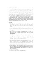
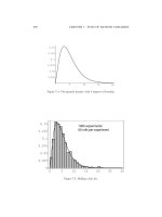
One program on the disk illustrates the central limit theorem. It considers random
variables that take on one of the values 0, 1, 2, 3, 4, and allows the user to enter the
probabilities for these values along with an integer n. The program then plots the probability
mass function of the sum of n independent random variables having this distribution. By
increasing n, one can “see” the mass function converge to the shape of a normal density
function.

ACKNOWLEDGEMENTS
We thank the following people for their helpful comments on the Third Edition:
•
•
•
•
•
•
•
•
•
•

Charles F. Dunkl, University of Virginia, Charlottesville
Gabor Szekely, Bowling Green State University
Krzysztof M. Ostaszewski, Illinois State University
Micael Ratliff, Northern Arizona University
Wei-Min Huang, Lehigh University
Youngho Lee, Howard University
Jacques Rioux, Drake University
Lisa Gardner, Bradley University

Murray Lieb, New Jersey Institute of Technology
Philip Trotter, Cornell University


This Page Intentionally Left Blank


Chapter 1

INTRODUCTION TO STATISTICS

1.1 INTRODUCTION
It has become accepted in today’s world that in order to learn about something, you must
first collect data. Statistics is the art of learning from data. It is concerned with the collection
of data, its subsequent description, and its analysis, which often leads to the drawing of
conclusions.

1.2 DATA COLLECTION AND DESCRIPTIVE STATISTICS
Sometimes a statistical analysis begins with a given set of data: For instance, the government
regularly collects and publicizes data concerning yearly precipitation totals, earthquake
occurrences, the unemployment rate, the gross domestic product, and the rate of inflation.
Statistics can be used to describe, summarize, and analyze these data.
In other situations, data are not yet available; in such cases statistical theory can be used to
design an appropriate experiment to generate data. The experiment chosen should depend
on the use that one wants to make of the data. For instance, suppose that an instructor is interested in determining which of two different methods for teaching computer
programming to beginners is most effective. To study this question, the instructor might
divide the students into two groups, and use a different teaching method for each group.
At the end of the class the students can be tested and the scores of the members of the
different groups compared. If the data, consisting of the test scores of members of each
group, are significantly higher in one of the groups, then it might seem reasonable to

suppose that the teaching method used for that group is superior.
It is important to note, however, that in order to be able to draw a valid conclusion
from the data, it is essential that the students were divided into groups in such a manner
that neither group was more likely to have the students with greater natural aptitude for
programming. For instance, the instructor should not have let the male class members be
one group and the females the other. For if so, then even if the women scored significantly
higher than the men, it would not be clear whether this was due to the method used
to teach them, or to the fact that women may be inherently better than men at learning
1


2

Chapter 1: Introduction to Statistics

programming skills. The accepted way of avoiding this pitfall is to divide the class members
into the two groups “at random.” This term means that the division is done in such
a manner that all possible choices of the members of a group are equally likely.
At the end of the experiment, the data should be described. For instance, the scores
of the two groups should be presented. In addition, summary measures such as the average score of members of each of the groups should be presented. This part of statistics,
concerned with the description and summarization of data, is called descriptive statistics.

1.3 INFERENTIAL STATISTICS AND
PROBABILITY MODELS
After the preceding experiment is completed and the data are described and summarized,
we hope to be able to draw a conclusion about which teaching method is superior. This
part of statistics, concerned with the drawing of conclusions, is called inferential statistics.
To be able to draw a conclusion from the data, we must take into account the possibility
of chance. For instance, suppose that the average score of members of the first group is
quite a bit higher than that of the second. Can we conclude that this increase is due to the

teaching method used? Or is it possible that the teaching method was not responsible for
the increased scores but rather that the higher scores of the first group were just a chance
occurrence? For instance, the fact that a coin comes up heads 7 times in 10 flips does
not necessarily mean that the coin is more likely to come up heads than tails in future
flips. Indeed, it could be a perfectly ordinary coin that, by chance, just happened to land
heads 7 times out of the total of 10 flips. (On the other hand, if the coin had landed
heads 47 times out of 50 flips, then we would be quite certain that it was not an ordinary
coin.)
To be able to draw logical conclusions from data, we usually make some assumptions
about the chances (or probabilities) of obtaining the different data values. The totality of
these assumptions is referred to as a probability model for the data.
Sometimes the nature of the data suggests the form of the probability model that is
assumed. For instance, suppose that an engineer wants to find out what proportion of
computer chips, produced by a new method, will be defective. The engineer might select
a group of these chips, with the resulting data being the number of defective chips in this
group. Provided that the chips selected were “randomly” chosen, it is reasonable to suppose
that each one of them is defective with probability p, where p is the unknown proportion
of all the chips produced by the new method that will be defective. The resulting data can
then be used to make inferences about p.
In other situations, the appropriate probability model for a given data set will not be
readily apparent. However, careful description and presentation of the data sometimes
enable us to infer a reasonable model, which we can then try to verify with the use of
additional data.
Because the basis of statistical inference is the formulation of a probability model to
describe the data, an understanding of statistical inference requires some knowledge of


1.5 A Brief History of Statistics

3

the theory of probability. In other words, statistical inference starts with the assumption
that important aspects of the phenomenon under study can be described in terms of
probabilities; it then draws conclusions by using data to make inferences about these
probabilities.

1.4 POPULATIONS AND SAMPLES
In statistics, we are interested in obtaining information about a total collection of elements,
which we will refer to as the population. The population is often too large for us to examine
each of its members. For instance, we might have all the residents of a given state, or all the
television sets produced in the last year by a particular manufacturer, or all the households
in a given community. In such cases, we try to learn about the population by choosing
and then examining a subgroup of its elements. This subgroup of a population is called
a sample.
If the sample is to be informative about the total population, it must be, in some sense,
representative of that population. For instance, suppose that we are interested in learning
about the age distribution of people residing in a given city, and we obtain the ages of the
first 100 people to enter the town library. If the average age of these 100 people is 46.2
years, are we justified in concluding that this is approximately the average age of the entire
population? Probably not, for we could certainly argue that the sample chosen in this case
is probably not representative of the total population because usually more young students
and senior citizens use the library than do working-age citizens.
In certain situations, such as the library illustration, we are presented with a sample and
must then decide whether this sample is reasonably representative of the entire population.
In practice, a given sample generally cannot be assumed to be representative of a population
unless that sample has been chosen in a random manner. This is because any specific
nonrandom rule for selecting a sample often results in one that is inherently biased toward
some data values as opposed to others.
Thus, although it may seem paradoxical, we are most likely to obtain a representative
sample by choosing its members in a totally random fashion without any prior considerations of the elements that will be chosen. In other words, we need not attempt to

deliberately choose the sample so that it contains, for instance, the same gender percentage
and the same percentage of people in each profession as found in the general population.
Rather, we should just leave it up to “chance” to obtain roughly the correct percentages.
Once a random sample is chosen, we can use statistical inference to draw conclusions about
the entire population by studying the elements of the sample.

1.5 A BRIEF HISTORY OF STATISTICS
A systematic collection of data on the population and the economy was begun in the Italian
city states of Venice and Florence during the Renaissance. The term statistics, derived from
the word state, was used to refer to a collection of facts of interest to the state. The idea of


4

Chapter 1: Introduction to Statistics

collecting data spread from Italy to the other countries of Western Europe. Indeed, by the
first half of the 16th century it was common for European governments to require parishes
to register births, marriages, and deaths. Because of poor public health conditions this last
statistic was of particular interest.
The high mortality rate in Europe before the 19th century was due mainly to epidemic
diseases, wars, and famines. Among epidemics, the worst were the plagues. Starting with
the Black Plague in 1348, plagues recurred frequently for nearly 400 years. In 1562, as a
way to alert the King’s court to consider moving to the countryside, the City of London
began to publish weekly bills of mortality. Initially these mortality bills listed the places
of death and whether a death had resulted from plague. Beginning in 1625 the bills were
expanded to include all causes of death.
In 1662 the English tradesman John Graunt published a book entitled Natural and
Political Observations Made upon the Bills of Mortality. Table 1.1, which notes the total
number of deaths in England and the number due to the plague for five different plague

years, is taken from this book.
TABLE 1.1

Total Deaths in England

Year

Burials

Plague Deaths

1592
1593
1603
1625
1636

25,886
17,844
37,294
51,758
23,359

11,503
10,662
30,561
35,417
10,400

Source: John Graunt, Observations Made upon the Bills of Mortality.

3rd ed. London: John Martyn and James Allestry (1st ed. 1662).

Graunt used London bills of mortality to estimate the city’s population. For instance,
to estimate the population of London in 1660, Graunt surveyed households in certain
London parishes (or neighborhoods) and discovered that, on average, there were approximately 3 deaths for every 88 people. Dividing by 3 shows that, on average, there was
roughly 1 death for every 88/3 people. Because the London bills cited 13,200 deaths in
London for that year, Graunt estimated the London population to be about
13,200 × 88/3 = 387,200
Graunt used this estimate to project a figure for all England. In his book he noted that
these figures would be of interest to the rulers of the country, as indicators of both the
number of men who could be drafted into an army and the number who could be taxed.
Graunt also used the London bills of mortality — and some intelligent guesswork as to
what diseases killed whom and at what age — to infer ages at death. (Recall that the bills
of mortality listed only causes and places at death, not the ages of those dying.) Graunt
then used this information to compute tables giving the proportion of the population that


1.5 A Brief History of Statistics

TABLE 1.2

5

John Graunt’s Mortality Table

Age at Death

Number of Deaths per 100 Births

0–6

6–16
16–26
26–36
36–46
46–56
56–66
66–76
76 and greater

36
24
15
9
6
4
3
2
1

Note: The categories go up to but do not include the right-hand value. For instance,
0–6 means all ages from 0 up through 5.

dies at various ages. Table 1.2 is one of Graunt’s mortality tables. It states, for instance,
that of 100 births, 36 people will die before reaching age 6, 24 will die between the age of
6 and 15, and so on.
Graunt’s estimates of the ages at which people were dying were of great interest to those
in the business of selling annuities. Annuities are the opposite of life insurance in that one
pays in a lump sum as an investment and then receives regular payments for as long as one
lives.
Graunt’s work on mortality tables inspired further work by Edmund Halley in 1693.

Halley, the discoverer of the comet bearing his name (and also the man who was most
responsible, by both his encouragement and his financial support, for the publication of
Isaac Newton’s famous Principia Mathematica), used tables of mortality to compute the
odds that a person of any age would live to any other particular age. Halley was influential
in convincing the insurers of the time that an annual life insurance premium should depend
on the age of the person being insured.
Following Graunt and Halley, the collection of data steadily increased throughout
the remainder of the 17th and on into the 18th century. For instance, the city of Paris
began collecting bills of mortality in 1667; and by 1730 it had become common practice
throughout Europe to record ages at death.
The term statistics, which was used until the 18th century as a shorthand for the
descriptive science of states, became in the 19th century increasingly identified with
numbers. By the 1830s the term was almost universally regarded in Britain and France
as being synonymous with the “numerical science” of society. This change in meaning
was caused by the large availability of census records and other tabulations that began to
be systematically collected and published by the governments of Western Europe and the
United States beginning around 1800.
Throughout the 19th century, although probability theory had been developed by such
mathematicians as Jacob Bernoulli, Karl Friedrich Gauss, and Pierre-Simon Laplace, its
use in studying statistical findings was almost nonexistent, because most social statisticians


6

Chapter 1: Introduction to Statistics

at the time were content to let the data speak for themselves. In particular, statisticians
of that time were not interested in drawing inferences about individuals, but rather were
concerned with the society as a whole. Thus, they were not concerned with sampling but
rather tried to obtain censuses of the entire population. As a result, probabilistic inference

from samples to a population was almost unknown in 19th century social statistics.
It was not until the late 1800s that statistics became concerned with inferring conclusions
from numerical data. The movement began with Francis Galton’s work on analyzing
hereditary genius through the uses of what we would now call regression and correlation
analysis (see Chapter 9), and obtained much of its impetus from the work of Karl Pearson.
Pearson, who developed the chi-square goodness of fit tests (see Chapter 11), was the first
director of the Galton Laboratory, endowed by Francis Galton in 1904. There Pearson
originated a research program aimed at developing new methods of using statistics in
inference. His laboratory invited advanced students from science and industry to learn
statistical methods that could then be applied in their fields. One of his earliest visiting
researchers was W. S. Gosset, a chemist by training, who showed his devotion to Pearson
by publishing his own works under the name “Student.” (A famous story has it that Gosset
was afraid to publish under his own name for fear that his employers, the Guinness brewery,
would be unhappy to discover that one of its chemists was doing research in statistics.)
Gosset is famous for his development of the t-test (see Chapter 8).
Two of the most important areas of applied statistics in the early 20th century were
population biology and agriculture. This was due to the interest of Pearson and others at
his laboratory and also to the remarkable accomplishments of the English scientist Ronald
A. Fisher. The theory of inference developed by these pioneers, including among others

TABLE 1.3

The Changing Definition of Statistics

Statistics has then for its object that of presenting a faithful representation of a state at a determined
epoch. (Quetelet, 1849)
Statistics are the only tools by which an opening can be cut through the formidable thicket of
difficulties that bars the path of those who pursue the Science of man. (Galton, 1889)
Statistics may be regarded (i) as the study of populations, (ii) as the study of variation, and (iii) as the
study of methods of the reduction of data. (Fisher, 1925)

Statistics is a scientific discipline concerned with collection, analysis, and interpretation of data obtained
from observation or experiment. The subject has a coherent structure based on the theory of
Probability and includes many different procedures which contribute to research and development
throughout the whole of Science and Technology. (E. Pearson, 1936)
Statistics is the name for that science and art which deals with uncertain inferences — which uses
numbers to find out something about nature and experience. (Weaver, 1952)
Statistics has become known in the 20th century as the mathematical tool for analyzing experimental
and observational data. (Porter, 1986)
Statistics is the art of learning from data. (this book, 2004)


Problems

7

Karl Pearson’s son Egon and the Polish born mathematical statistician Jerzy Neyman,
was general enough to deal with a wide range of quantitative and practical problems. As
a result, after the early years of the 20th century a rapidly increasing number of people
in science, business, and government began to regard statistics as a tool that was able to
provide quantitative solutions to scientific and practical problems (see Table 1.3).
Nowadays the ideas of statistics are everywhere. Descriptive statistics are featured in
every newspaper and magazine. Statistical inference has become indispensable to public
health and medical research, to engineering and scientific studies, to marketing and quality
control, to education, to accounting, to economics, to meteorological forecasting, to
polling and surveys, to sports, to insurance, to gambling, and to all research that makes
any claim to being scientific. Statistics has indeed become ingrained in our intellectual
heritage.

Problems
1. An election will be held next week and, by polling a sample of the voting

population, we are trying to predict whether the Republican or Democratic
candidate will prevail. Which of the following methods of selection is likely to
yield a representative sample?
(a) Poll all people of voting age attending a college basketball game.
(b) Poll all people of voting age leaving a fancy midtown restaurant.
(c) Obtain a copy of the voter registration list, randomly choose 100 names, and
question them.
(d) Use the results of a television call-in poll, in which the station asked its listeners
to call in and name their choice.
(e) Choose names from the telephone directory and call these people.
2. The approach used in Problem 1(e) led to a disastrous prediction in the 1936
presidential election, in which Franklin Roosevelt defeated Alfred Landon by a
landslide. A Landon victory had been predicted by the Literary Digest. The magazine based its prediction on the preferences of a sample of voters chosen from lists
of automobile and telephone owners.
(a) Why do you think the Literary Digest’s prediction was so far off?
(b) Has anything changed between 1936 and now that would make you believe
that the approach used by the Literary Digest would work better today?
3. A researcher is trying to discover the average age at death for people in the United
States today. To obtain data, the obituary columns of the New York Times are read
for 30 days, and the ages at death of people in the United States are noted. Do
you think this approach will lead to a representative sample?


8

Chapter 1: Introduction to Statistics

4. To determine the proportion of people in your town who are smokers, it has been
decided to poll people at one of the following local spots:
(a)

(b)
(c)
(d)

the pool hall;
the bowling alley;
the shopping mall;
the library.

Which of these potential polling places would most likely result in a reasonable
approximation to the desired proportion? Why?
5. A university plans on conducting a survey of its recent graduates to determine
information on their yearly salaries. It randomly selected 200 recent graduates and
sent them questionnaires dealing with their present jobs. Of these 200, however,
only 86 were returned. Suppose that the average of the yearly salaries reported was
$75,000.
(a) Would the university be correct in thinking that $75,000 was a good approximation to the average salary level of all of its graduates? Explain the reasoning
behind your answer.
(b) If your answer to part (a) is no, can you think of any set of conditions relating to the group that returned questionnaires for which it would be a good
approximation?
6. An article reported that a survey of clothing worn by pedestrians killed at night in
traffic accidents revealed that about 80 percent of the victims were wearing darkcolored clothing and 20 percent were wearing light-colored clothing. The conclusion drawn in the article was that it is safer to wear light-colored clothing at night.
(a) Is this conclusion justified? Explain.
(b) If your answer to part (a) is no, what other information would be needed
before a final conclusion could be drawn?
7. Critique Graunt’s method for estimating the population of London. What
implicit assumption is he making?
8. The London bills of mortality listed 12,246 deaths in 1658. Supposing that a
survey of London parishes showed that roughly 2 percent of the population died
that year, use Graunt’s method to estimate London’s population in 1658.

9. Suppose you were a seller of annuities in 1662 when Graunt’s book was published.
Explain how you would make use of his data on the ages at which people were
dying.
10. Based on Graunt’s mortality table:
(a) What proportion of people survived to age 6?
(b) What proportion survived to age 46?
(c) What proportion died between the ages of 6 and 36?