Statistics with STATA version 12
Bạn đang xem bản rút gọn của tài liệu. Xem và tải ngay bản đầy đủ của tài liệu tại đây (13.67 MB, 488 trang )
Copyright 2012 Cengage Learning. All Rights Reserved. May not be copied, scanned, or duplicated, in whole or in part. Due to electronic rights, some third party content may be suppressed from the eBook and/or eChapter(s). Editorial review has
deemed that any suppressed content does not materially affect the overall learning experience. Cengage Learning reserves the right to remove additional content at any time if subsequent rights restrictions require it.
Statistics
with
STATA
Updated for Version 12
Copyright 2012 Cengage Learning. All Rights Reserved. May not be copied, scanned, or duplicated, in whole or in part. Due to electronic rights, some third party content may be suppressed from the eBook and/or eChapter(s). Editorial review has
deemed that any suppressed content does not materially affect the overall learning experience. Cengage Learning reserves the right to remove additional content at any time if subsequent rights restrictions require it.
This is an electronic version of the print textbook. Due to electronic rights restrictions, some third party content may be suppressed. Editorial
review has deemed that any suppressed content does not materially affect the overall learning experience. The publisher reserves the right to
remove content from this title at any time if subsequent rights restrictions require it. For valuable information on pricing, previous
editions, changes to current editions, and alternate formats, please visit www.cengage.com/highered to search by
ISBN#, author, title, or keyword for materials in your areas of interest.
Copyright 2012 Cengage Learning. All Rights Reserved. May not be copied, scanned, or duplicated, in whole or in part. Due to electronic rights, some third party content may be suppressed from the eBook and/or eChapter(s). Editorial review has
deemed that any suppressed content does not materially affect the overall learning experience. Cengage Learning reserves the right to remove additional content at any time if subsequent rights restrictions require it.
Statistics
with
STATA
Updated for Version 12
Lawrence C. Hamilton
University of New Hampshire
Australia • Brazil • Japan • Korea • Mexico • Singapore • Spain • United Kingdom • United States
Copyright 2012 Cengage Learning. All Rights Reserved. May not be copied, scanned, or duplicated, in whole or in part. Due to electronic rights, some third party content may be suppressed from the eBook and/or eChapter(s). Editorial review has
deemed that any suppressed content does not materially affect the overall learning experience. Cengage Learning reserves the right to remove additional content at any time if subsequent rights restrictions require it.
Statistics with STATA: Updated for Version 12
©
Eighth Edition
ALL RIGHTS RESERVED. No part of this work covered by the copyright
herein may be reproduced, transmitted, stored, or used in any form or by
any means graphic, electronic, or mechanical, including but not limited to
photocopying, recording, scanning, digitizing, taping, Web distribution, information networks, or information storage and retrieval systems, except as
permitted under Section 107 or 108 of the 1976 United States Copyright Act,
without the prior written permission of the publisher.
Lawrence C. Hamilton
Publisher/Executive Editor: Richard Stratton
Senior Sponsoring Editor: Molly Taylor
Assistant Editor: Shaylin Walsh Hogan
Editorial Assistant/Associate: Alexander Gontar
Media Editor: Andrew Coppola
Marketing Assistant: Lauren Beck
Marketing Communications Manager:
Jason LaChappelle
, 2009, 2006 Brooks/Cole, Cengage Learning
For product information and technology assistance, contact us at
Cengage Learning Customer & Sales Support, 1-800-354-9706
For permission to use material from this text or product,
submit all requests online at www.cengage.com/permissions.
Further permissions questions can be emailed to
Library of Congress Control Number: 2012945319
ISBN-13: 978-0-8400-6463-9
ISBN-10: 0-8400-6463-2
Brooks/
k Cole
20 Channel Center Street
Boston, MA 02210
USA
Cengage Learning is a leading provider of customized learning solutions with
offi
ffice locations around the globe, including Singapore, the United Kingdom,
Australia, Mexico, Brazil and Japan. Locate your local office
ffi at
international.cengage.com/region
Cengage Learning products are represented in Canada by
Nelson Education, Ltd.
For your course and learning solutions, visit www.cengage.com.
Purchase any of our products at your local college store or at our preferred
online store www.cengagebrain.com.
Instructors: Please visit login.cengage.com and log in to access
instructor-specific
fi resources.
Printed in the United States of America
1 2 3 4 5 6 7 16 15 14 13 12
Copyright 2012 Cengage Learning. All Rights Reserved. May not be copied, scanned, or duplicated, in whole or in part. Due to electronic rights, some third party content may be suppressed from the eBook and/or eChapter(s). Editorial review has
deemed that any suppressed content does not materially affect the overall learning experience. Cengage Learning reserves the right to remove additional content at any time if subsequent rights restrictions require it.
Contents
Preface . . . . . . . . . . . . . . . . . . . . . . . . . . . . . . . . . . . . . . . . . . . . . . . . . . . . . . . . . . ix
Notes on the Eighth Edition . . . . . . . . . . . . . . . . . . . . . . . . . . . . . . . . . . . . . . . . . . . x
Acknowledgments . . . . . . . . . . . . . . . . . . . . . . . . . . . . . . . . . . . . . . . . . . . . . . . . . . xi
1
Stata and Stata Resources . . . . . . . . . . . . . . . . . . . . . . . . . . . . . . . . . . . . . . . 1
A Typographical Note . . . . . . . . . . . . . . . . . . . . . . . . . . . . . . . . . . . . . . . . . . . . . . . . 1
An Example Stata Session . . . . . . . . . . . . . . . . . . . . . . . . . . . . . . . . . . . . . . . . . . . . 2
Stata’s Documentation and Help Files . . . . . . . . . . . . . . . . . . . . . . . . . . . . . . . . . . . 7
Searching for Information . . . . . . . . . . . . . . . . . . . . . . . . . . . . . . . . . . . . . . . . . . . . . 8
StataCorp . . . . . . . . . . . . . . . . . . . . . . . . . . . . . . . . . . . . . . . . . . . . . . . . . . . . . . . . . . 9
The Stata Journal . . . . . . . . . . . . . . . . . . . . . . . . . . . . . . . . . . . . . . . . . . . . . . . . . . 10
Books Using Stata . . . . . . . . . . . . . . . . . . . . . . . . . . . . . . . . . . . . . . . . . . . . . . . . . . 11
2
Data Management . . . . . . . . . . . . . . . . . . . . . . . . . . . . . . . . . . . . . . . . . . . . . .
Example Commands . . . . . . . . . . . . . . . . . . . . . . . . . . . . . . . . . . . . . . . . . . . . . . . .
Creating a New Dataset by Typing in Data . . . . . . . . . . . . . . . . . . . . . . . . . . . . . .
Creating a New Dataset by Copy and Paste . . . . . . . . . . . . . . . . . . . . . . . . . . . . . .
Specifying Subsets of the Data: in and if Qualifiers . . . . . . . . . . . . . . . . . . . . . . .
Generating and Replacing Variables . . . . . . . . . . . . . . . . . . . . . . . . . . . . . . . . . . . .
Missing Value Codes . . . . . . . . . . . . . . . . . . . . . . . . . . . . . . . . . . . . . . . . . . . . . . .
Using Functions . . . . . . . . . . . . . . . . . . . . . . . . . . . . . . . . . . . . . . . . . . . . . . . . . . .
Converting Between Numeric and String Formats . . . . . . . . . . . . . . . . . . . . . . . . .
Creating New Categorical and Ordinal Variables . . . . . . . . . . . . . . . . . . . . . . . . . .
Using Explicit Subscripts with Variables . . . . . . . . . . . . . . . . . . . . . . . . . . . . . . . .
Importing Data from Other Programs . . . . . . . . . . . . . . . . . . . . . . . . . . . . . . . . . . .
Combining Two or More Stata Files . . . . . . . . . . . . . . . . . . . . . . . . . . . . . . . . . . . .
Collapsing Data . . . . . . . . . . . . . . . . . . . . . . . . . . . . . . . . . . . . . . . . . . . . . . . . . . . .
Reshaping Data . . . . . . . . . . . . . . . . . . . . . . . . . . . . . . . . . . . . . . . . . . . . . . . . . . . .
Using Weights . . . . . . . . . . . . . . . . . . . . . . . . . . . . . . . . . . . . . . . . . . . . . . . . . . . . .
Creating Random Data and Random Samples . . . . . . . . . . . . . . . . . . . . . . . . . . . .
Writing Programs for Data Management . . . . . . . . . . . . . . . . . . . . . . . . . . . . . . . .
13
14
16
21
23
26
29
32
36
39
41
42
46
49
52
55
57
61
3
Graphs . . . . . . . . . . . . . . . . . . . . . . . . . . . . . . . . . . . . . . . . . . . . . . . . . . . . . . .
Example Commands . . . . . . . . . . . . . . . . . . . . . . . . . . . . . . . . . . . . . . . . . . . . . . . .
Histograms . . . . . . . . . . . . . . . . . . . . . . . . . . . . . . . . . . . . . . . . . . . . . . . . . . . . . . .
Box Plots . . . . . . . . . . . . . . . . . . . . . . . . . . . . . . . . . . . . . . . . . . . . . . . . . . . . . . . .
Scatterplots and Overlays . . . . . . . . . . . . . . . . . . . . . . . . . . . . . . . . . . . . . . . . . . . .
Line Plots and Connected-Line Plots . . . . . . . . . . . . . . . . . . . . . . . . . . . . . . . . . . .
Other Twoway Plot Types . . . . . . . . . . . . . . . . . . . . . . . . . . . . . . . . . . . . . . . . . . .
65
65
68
71
74
80
85
v
Copyright 2012 Cengage Learning. All Rights Reserved. May not be copied, scanned, or duplicated, in whole or in part. Due to electronic rights, some third party content may be suppressed from the eBook and/or eChapter(s). Editorial review has
deemed that any suppressed content does not materially affect the overall learning experience. Cengage Learning reserves the right to remove additional content at any time if subsequent rights restrictions require it.
vi
Statistics with Stata
Bar Charts and Pie Charts . . . . . . . . . . . . . . . . . . . . . . . . . . . . . . . . . . . . . . . . . . . . 87
Symmetry and Quantile Plots . . . . . . . . . . . . . . . . . . . . . . . . . . . . . . . . . . . . . . . . . 90
Adding Text to Graphs . . . . . . . . . . . . . . . . . . . . . . . . . . . . . . . . . . . . . . . . . . . . . . 93
Graphing with Do-Files . . . . . . . . . . . . . . . . . . . . . . . . . . . . . . . . . . . . . . . . . . . . . 95
Retrieving and Combining Graphs . . . . . . . . . . . . . . . . . . . . . . . . . . . . . . . . . . . . . 96
Graph Editor . . . . . . . . . . . . . . . . . . . . . . . . . . . . . . . . . . . . . . . . . . . . . . . . . . . . . . 97
Creative Graphing . . . . . . . . . . . . . . . . . . . . . . . . . . . . . . . . . . . . . . . . . . . . . . . . . 100
4
Survey Data . . . . . . . . . . . . . . . . . . . . . . . . . . . . . . . . . . . . . . . . . . . . . . . . . 107
Example Commands . . . . . . . . . . . . . . . . . . . . . . . . . . . . . . . . . . . . . . . . . . . . . . . 108
Declare Survey Data . . . . . . . . . . . . . . . . . . . . . . . . . . . . . . . . . . . . . . . . . . . . . . . 108
Design Weights . . . . . . . . . . . . . . . . . . . . . . . . . . . . . . . . . . . . . . . . . . . . . . . . . . . 110
Poststratification Weights . . . . . . . . . . . . . . . . . . . . . . . . . . . . . . . . . . . . . . . . . . . 113
Survey-Weighted Tables and Graphs . . . . . . . . . . . . . . . . . . . . . . . . . . . . . . . . . . 115
Bar Charts for Multiple Comparisons . . . . . . . . . . . . . . . . . . . . . . . . . . . . . . . . . . 119
5
Summary Statistics and Tables . . . . . . . . . . . . . . . . . . . . . . . . . . . . . . . . . 123
Example Commands . . . . . . . . . . . . . . . . . . . . . . . . . . . . . . . . . . . . . . . . . . . . . . . 123
Summary Statistics for Measurement Variables . . . . . . . . . . . . . . . . . . . . . . . . . . 125
Exploratory Data Analysis . . . . . . . . . . . . . . . . . . . . . . . . . . . . . . . . . . . . . . . . . . 127
Normality Tests and Transformations . . . . . . . . . . . . . . . . . . . . . . . . . . . . . . . . . . 129
Frequency Tables and Two-Way Cross-Tabulations . . . . . . . . . . . . . . . . . . . . . . 133
Multiple Tables and Multi-Way Cross-Tabulations . . . . . . . . . . . . . . . . . . . . . . . 136
Tables of Means, Medians and Other Summary Statistics . . . . . . . . . . . . . . . . . . 139
Using Frequency Weights . . . . . . . . . . . . . . . . . . . . . . . . . . . . . . . . . . . . . . . . . . . 140
6
ANOVA and Other Comparison Methods . . . . . . . . . . . . . . . . . . . . . . . . . . 143
Example Commands . . . . . . . . . . . . . . . . . . . . . . . . . . . . . . . . . . . . . . . . . . . . . . . 144
One-Sample Tests . . . . . . . . . . . . . . . . . . . . . . . . . . . . . . . . . . . . . . . . . . . . . . . . . 145
Two-Sample Tests . . . . . . . . . . . . . . . . . . . . . . . . . . . . . . . . . . . . . . . . . . . . . . . . . 148
One-Way Analysis of Variance (ANOVA) . . . . . . . . . . . . . . . . . . . . . . . . . . . . . 151
Two- and N-Way Analysis of Variance . . . . . . . . . . . . . . . . . . . . . . . . . . . . . . . . 154
Factor Variables and Analysis of Covariance (ANCOVA) . . . . . . . . . . . . . . . . . 155
Predicted Values and Error-Bar Charts . . . . . . . . . . . . . . . . . . . . . . . . . . . . . . . . . 158
7
Linear Regression Analysis . . . . . . . . . . . . . . . . . . . . . . . . . . . . . . . . . . . . 163
Example Commands . . . . . . . . . . . . . . . . . . . . . . . . . . . . . . . . . . . . . . . . . . . . . . . 163
Simple Regression . . . . . . . . . . . . . . . . . . . . . . . . . . . . . . . . . . . . . . . . . . . . . . . . . 167
Correlation . . . . . . . . . . . . . . . . . . . . . . . . . . . . . . . . . . . . . . . . . . . . . . . . . . . . . . 170
Multiple Regression . . . . . . . . . . . . . . . . . . . . . . . . . . . . . . . . . . . . . . . . . . . . . . . 174
Hypothesis Tests . . . . . . . . . . . . . . . . . . . . . . . . . . . . . . . . . . . . . . . . . . . . . . . . . . 179
Dummy Variables . . . . . . . . . . . . . . . . . . . . . . . . . . . . . . . . . . . . . . . . . . . . . . . . . 181
Interaction Effects . . . . . . . . . . . . . . . . . . . . . . . . . . . . . . . . . . . . . . . . . . . . . . . . . 185
Robust Estimates of Variance . . . . . . . . . . . . . . . . . . . . . . . . . . . . . . . . . . . . . . . . 190
Predicted Values and Residuals . . . . . . . . . . . . . . . . . . . . . . . . . . . . . . . . . . . . . . 192
Other Case Statistics . . . . . . . . . . . . . . . . . . . . . . . . . . . . . . . . . . . . . . . . . . . . . . . 197
Diagnosing Multicollinearity and Heteroskedasticity . . . . . . . . . . . . . . . . . . . . . . 202
Copyright 2012 Cengage Learning. All Rights Reserved. May not be copied, scanned, or duplicated, in whole or in part. Due to electronic rights, some third party content may be suppressed from the eBook and/or eChapter(s). Editorial review has
deemed that any suppressed content does not materially affect the overall learning experience. Cengage Learning reserves the right to remove additional content at any time if subsequent rights restrictions require it.
Contents
vii
Confidence Bands in Simple Regression . . . . . . . . . . . . . . . . . . . . . . . . . . . . . . . 205
Diagnostic Graphs . . . . . . . . . . . . . . . . . . . . . . . . . . . . . . . . . . . . . . . . . . . . . . . . . 209
8
Advanced Regression Methods . . . . . . . . . . . . . . . . . . . . . . . . . . . . . . . . . 215
Example Commands . . . . . . . . . . . . . . . . . . . . . . . . . . . . . . . . . . . . . . . . . . . . . . . 215
Lowess Smoothing . . . . . . . . . . . . . . . . . . . . . . . . . . . . . . . . . . . . . . . . . . . . . . . . 217
Robust Regression . . . . . . . . . . . . . . . . . . . . . . . . . . . . . . . . . . . . . . . . . . . . . . . . 221
Further rreg and qreg Applications . . . . . . . . . . . . . . . . . . . . . . . . . . . . . . . . . . . 227
Nonlinear Regression — 1 . . . . . . . . . . . . . . . . . . . . . . . . . . . . . . . . . . . . . . . . . . 230
Nonlinear Regression — 2 . . . . . . . . . . . . . . . . . . . . . . . . . . . . . . . . . . . . . . . . . . 233
Box–Cox Regression . . . . . . . . . . . . . . . . . . . . . . . . . . . . . . . . . . . . . . . . . . . . . . 238
Multiple Imputation of Missing Values . . . . . . . . . . . . . . . . . . . . . . . . . . . . . . . . 241
Structural Equation Modeling . . . . . . . . . . . . . . . . . . . . . . . . . . . . . . . . . . . . . . . . 244
9
Logistic Regression . . . . . . . . . . . . . . . . . . . . . . . . . . . . . . . . . . . . . . . . . . . 251
Example Commands . . . . . . . . . . . . . . . . . . . . . . . . . . . . . . . . . . . . . . . . . . . . . . . 252
Space Shuttle Data . . . . . . . . . . . . . . . . . . . . . . . . . . . . . . . . . . . . . . . . . . . . . . . . 254
Using Logistic Regression . . . . . . . . . . . . . . . . . . . . . . . . . . . . . . . . . . . . . . . . . . 258
Marginal or Conditional Effects Plots . . . . . . . . . . . . . . . . . . . . . . . . . . . . . . . . . 262
Diagnostic Statistics and Plots . . . . . . . . . . . . . . . . . . . . . . . . . . . . . . . . . . . . . . . 264
Logistic Regression with Ordered-Category y . . . . . . . . . . . . . . . . . . . . . . . . . . . 268
Multinomial Logistic Regression . . . . . . . . . . . . . . . . . . . . . . . . . . . . . . . . . . . . . 270
Multiple Imputation of Missing Values — Logit Regression Example . . . . . . . . 278
10 Survival and Event-Count Models . . . . . . . . . . . . . . . . . . . . . . . . . . . . . . . . 283
Example Commands . . . . . . . . . . . . . . . . . . . . . . . . . . . . . . . . . . . . . . . . . . . . . . . 284
Survival-Time Data . . . . . . . . . . . . . . . . . . . . . . . . . . . . . . . . . . . . . . . . . . . . . . . . 286
Count-Time Data . . . . . . . . . . . . . . . . . . . . . . . . . . . . . . . . . . . . . . . . . . . . . . . . . . 288
Kaplan–Meier Survivor Functions . . . . . . . . . . . . . . . . . . . . . . . . . . . . . . . . . . . . 290
Cox Proportional Hazard Models . . . . . . . . . . . . . . . . . . . . . . . . . . . . . . . . . . . . . 293
Exponential and Weibull Regression . . . . . . . . . . . . . . . . . . . . . . . . . . . . . . . . . . 299
Poisson Regression . . . . . . . . . . . . . . . . . . . . . . . . . . . . . . . . . . . . . . . . . . . . . . . . 303
Generalized Linear Models . . . . . . . . . . . . . . . . . . . . . . . . . . . . . . . . . . . . . . . . . . 307
11 Principal Component, Factor and Cluster Analysis . . . . . . . . . . . . . . . . . 313
Example Commands . . . . . . . . . . . . . . . . . . . . . . . . . . . . . . . . . . . . . . . . . . . . . . . 314
Principal Component Analysis and Principal Component Factoring . . . . . . . . . . 315
Rotation . . . . . . . . . . . . . . . . . . . . . . . . . . . . . . . . . . . . . . . . . . . . . . . . . . . . . . . . . 318
Factor Scores . . . . . . . . . . . . . . . . . . . . . . . . . . . . . . . . . . . . . . . . . . . . . . . . . . . . . 321
Principal Factoring . . . . . . . . . . . . . . . . . . . . . . . . . . . . . . . . . . . . . . . . . . . . . . . . 323
Maximum-Likelihood Factoring . . . . . . . . . . . . . . . . . . . . . . . . . . . . . . . . . . . . . . 325
Cluster Analysis — 1 . . . . . . . . . . . . . . . . . . . . . . . . . . . . . . . . . . . . . . . . . . . . . . 327
Cluster Analysis — 2 . . . . . . . . . . . . . . . . . . . . . . . . . . . . . . . . . . . . . . . . . . . . . . 331
Using Factor Scores in Regression . . . . . . . . . . . . . . . . . . . . . . . . . . . . . . . . . . . . 336
Measurement and Structural Equation Models . . . . . . . . . . . . . . . . . . . . . . . . . . . 344
Copyright 2012 Cengage Learning. All Rights Reserved. May not be copied, scanned, or duplicated, in whole or in part. Due to electronic rights, some third party content may be suppressed from the eBook and/or eChapter(s). Editorial review has
deemed that any suppressed content does not materially affect the overall learning experience. Cengage Learning reserves the right to remove additional content at any time if subsequent rights restrictions require it.
viii
Statistics with Stata
12 Time Series Analysis . . . . . . . . . . . . . . . . . . . . . . . . . . . . . . . . . . . . . . . . . . 351
Example Commands . . . . . . . . . . . . . . . . . . . . . . . . . . . . . . . . . . . . . . . . . . . . . . . 351
Smoothing . . . . . . . . . . . . . . . . . . . . . . . . . . . . . . . . . . . . . . . . . . . . . . . . . . . . . . . 353
Further Time Plot Examples . . . . . . . . . . . . . . . . . . . . . . . . . . . . . . . . . . . . . . . . . 359
Recent Climate Change . . . . . . . . . . . . . . . . . . . . . . . . . . . . . . . . . . . . . . . . . . . . . 363
Lags, Lead and Differences . . . . . . . . . . . . . . . . . . . . . . . . . . . . . . . . . . . . . . . . . . 366
Correlograms . . . . . . . . . . . . . . . . . . . . . . . . . . . . . . . . . . . . . . . . . . . . . . . . . . . . . 371
ARIMA Models . . . . . . . . . . . . . . . . . . . . . . . . . . . . . . . . . . . . . . . . . . . . . . . . . . 374
ARMAX Models . . . . . . . . . . . . . . . . . . . . . . . . . . . . . . . . . . . . . . . . . . . . . . . . . . 382
13 Multilevel and Mixed-Effects Modeling . . . . . . . . . . . . . . . . . . . . . . . . . . . . 387
Example Commands . . . . . . . . . . . . . . . . . . . . . . . . . . . . . . . . . . . . . . . . . . . . . . . 388
Regression with Random Intercepts . . . . . . . . . . . . . . . . . . . . . . . . . . . . . . . . . . . 390
Random Intercepts and Slopes . . . . . . . . . . . . . . . . . . . . . . . . . . . . . . . . . . . . . . . 395
Multiple Random Slopes . . . . . . . . . . . . . . . . . . . . . . . . . . . . . . . . . . . . . . . . . . . . 400
Nested Levels . . . . . . . . . . . . . . . . . . . . . . . . . . . . . . . . . . . . . . . . . . . . . . . . . . . . 404
Repeated Measurements . . . . . . . . . . . . . . . . . . . . . . . . . . . . . . . . . . . . . . . . . . . . 406
Cross-Sectional Time Series . . . . . . . . . . . . . . . . . . . . . . . . . . . . . . . . . . . . . . . . . 410
Mixed-Effects Logit Regression . . . . . . . . . . . . . . . . . . . . . . . . . . . . . . . . . . . . . . 415
14 Introduction to Programming . . . . . . . . . . . . . . . . . . . . . . . . . . . . . . . . . . . 423
Basic Concepts and Tools . . . . . . . . . . . . . . . . . . . . . . . . . . . . . . . . . . . . . . . . . . . 423
Do-files . . . . . . . . . . . . . . . . . . . . . . . . . . . . . . . . . . . . . . . . . . . . . . . . . . . . . . 423
Ado-files . . . . . . . . . . . . . . . . . . . . . . . . . . . . . . . . . . . . . . . . . . . . . . . . . . . . . 424
Programs . . . . . . . . . . . . . . . . . . . . . . . . . . . . . . . . . . . . . . . . . . . . . . . . . . . . . 425
Local macros . . . . . . . . . . . . . . . . . . . . . . . . . . . . . . . . . . . . . . . . . . . . . . . . . 426
Global macros . . . . . . . . . . . . . . . . . . . . . . . . . . . . . . . . . . . . . . . . . . . . . . . . . 427
Scalars . . . . . . . . . . . . . . . . . . . . . . . . . . . . . . . . . . . . . . . . . . . . . . . . . . . . . . 427
Version . . . . . . . . . . . . . . . . . . . . . . . . . . . . . . . . . . . . . . . . . . . . . . . . . . . . . . 427
Comments . . . . . . . . . . . . . . . . . . . . . . . . . . . . . . . . . . . . . . . . . . . . . . . . . . . . 428
Looping . . . . . . . . . . . . . . . . . . . . . . . . . . . . . . . . . . . . . . . . . . . . . . . . . . . . . 429
If ... else . . . . . . . . . . . . . . . . . . . . . . . . . . . . . . . . . . . . . . . . . . . . . . . . . . . . . 430
Arguments . . . . . . . . . . . . . . . . . . . . . . . . . . . . . . . . . . . . . . . . . . . . . . . . . . . 431
Syntax . . . . . . . . . . . . . . . . . . . . . . . . . . . . . . . . . . . . . . . . . . . . . . . . . . . . . . . 432
Example Program: multicat (Plot Many Categorical Variables) . . . . . . . . . . . . 434
Using multicat . . . . . . . . . . . . . . . . . . . . . . . . . . . . . . . . . . . . . . . . . . . . . . . . . . . 437
Help File . . . . . . . . . . . . . . . . . . . . . . . . . . . . . . . . . . . . . . . . . . . . . . . . . . . . . . . . 441
Monte Carlo Simulation . . . . . . . . . . . . . . . . . . . . . . . . . . . . . . . . . . . . . . . . . . . . 445
Matrix Programming with Mata . . . . . . . . . . . . . . . . . . . . . . . . . . . . . . . . . . . . . . 452
Dataset Sources . . . . . . . . . . . . . . . . . . . . . . . . . . . . . . . . . . . . . . . . . . . . . . . . . 457
References . . . . . . . . . . . . . . . . . . . . . . . . . . . . . . . . . . . . . . . . . . . . . . . . . . . . . 461
Index . . . . . . . . . . . . . . . . . . . . . . . . . . . . . . . . . . . . . . . . . . . . . . . . . . . . . . . . . . 469
Copyright 2012 Cengage Learning. All Rights Reserved. May not be copied, scanned, or duplicated, in whole or in part. Due to electronic rights, some third party content may be suppressed from the eBook and/or eChapter(s). Editorial review has
deemed that any suppressed content does not materially affect the overall learning experience. Cengage Learning reserves the right to remove additional content at any time if subsequent rights restrictions require it.
Preface
Statistics with Stata is intended for students and practicing researchers, to bridge the gap
between statistical textbooks and Stata’s own documentation. In this intermediate role, it does
not provide the detailed expositions of a proper textbook, nor does it come close to describing
all of Stata’s features. Instead, it demonstrates how to use Stata to accomplish a wide variety of
statistical tasks. Chapter topics follow conceptual themes rather than focusing on particular Stata
commands, which gives Statistics with Stata a different structure from the Stata reference
manuals. The chapter on Data Management, for example, covers many different procedures for
creating, importing, combining or restructuring data files. Chapters on Graphs, Summary
Statistics and Tables, and on ANOVA and Other Comparison Methods have similarly broad
themes that encompass a number of separate techniques. A new chapter that introduces Survey
Data, placed early in the book, provides background for more technical survey examples
presented where appropriate in later chapters.
The general topics of the first seven chapters (through Linear Regression Analysis) roughly
parallel an undergraduate or first graduate-level course in applied statistics, but with additional
depth to cover practical issues often encountered by analysts — how to import datasets, draw
publication-quality graphics, work with survey weights, or do trouble-shooting in regression,
for instance. In Chapter 8 (Advanced Regression Methods) and beyond, we move into the
territory of advanced courses or original research. Here, readers can find basic information and
illustrations of lowess, robust, quantile, nonlinear, logit, ordered logit, multinomial logit or
Poisson regression; apply new methods for structural equation modeling or multiple imputation
of missing values; fit survival-time and event-count models; construct and use composite
variables from factor analysis or principal components; divide observations into empirical types
or clusters; analyze simple or multiple time series; and fit multilevel or mixed-effects models.
Stata has worked hard in recent years to advance its state-of-the-art standing, and this effort is
particularly apparent in the wide range of statistical modeling commands it now offers.
The book concludes with a look at programming in Stata. Many readers will find that Stata does
everything they need already, so they have no reason to write original programs. For an active
minority, however, programmability is one of Stata’s principal attractions, and it underlies
Stata’s currency and rapid advancement. Chapter 14 opens the door for new users to explore
Stata programming, whether for specialized data management tasks, to establish a new statistical
capability, for Monte Carlo experiments or for teaching.
Generally similar versions (“flavors”) of Stata run on Windows, Mac and Unix computers.
Across all platforms, Stata uses the same commands and produces the same output. Datasets,
graphs and programs created on one platform can be used by Stata running on any other
platform. The flavors differ in some details of screen appearance, menus and file handling,
where Stata follows the conventions native to each platform — such as \directory\filename file
specifications under Windows, in contrast with the /directory/filename specifications under
ix
Copyright 2012 Cengage Learning. All Rights Reserved. May not be copied, scanned, or duplicated, in whole or in part. Due to electronic rights, some third party content may be suppressed from the eBook and/or eChapter(s). Editorial review has
deemed that any suppressed content does not materially affect the overall learning experience. Cengage Learning reserves the right to remove additional content at any time if subsequent rights restrictions require it.
x
Statistics with Stata
Unix. Rather than display all three, I employ Windows conventions, but users with other
systems should find that only minor translations are needed.
Notes on the Eighth Edition
I began using Stata in 1985, the first year of its release. Initially, Stata ran only on MS-DOS
personal computers, but its desktop orientation made it distinctly more modern than its main
competitors — most of which had originated before the desktop revolution, in the 80-column
punched-card Fortran environment of mainframes. Unlike mainframe statistical packages that
believed each user was a stack of cards, Stata viewed the user as a conversation. Its interactive
nature and integration of statistical procedures with data management and graphics supported
the natural flow of analytical thought in ways that other programs did not. graph and predict
soon became favorite commands. I was impressed enough by how it all fit together to start
writing the first external Stata book, Statistics with Stata, published in 1989 for Stata version
2. Stata’s 20th anniversary in 2005 was marked by a special issue of the Stata Journal, filled
with historical articles, interviews and by invitation a brief history of Statistics with Stata.
A great deal about Stata has changed since this book’s first edition, in which I observed that
“Stata is not a do-everything program . . . . The things it does, however, it does very well.” The
expansion of Stata’s capabilities has been striking. This is very noticeable in the proliferation,
and later in the steady rationalization, of model fitting procedures. William Gould’s architecture
for Stata, with its programming tools and unified syntax, has aged well and smoothly
incorporated new statistical methods as these were developed. The broad range of graphs in
Chapter 3, the formidable list of modeling commands that begins Chapter 8, or the new time
series, survey, multiple-imputation or mixed-modeling capabilities discussed in later chapters
illustrate some of the ways that Stata became richer over the years. Suites of new techniques
such as those for panel (xt), survey (svy), time series (ts), survival time (st) or multiple
imputation (mi) data open worlds of possibility, as do programmable commands for generalized
linear modeling (glm), or general procedures for maximum-likelihood estimation. Other major
extensions include the development of a matrix programming capability, the wealth of new datamanagement features, and new multipurpose analytical tools such as marginal plots or structural
equation modeling. Data management, with good reason, has been promoted from an incidental
topic in the first Statistics with Stata to the longest chapter in this eighth edition.
Stata’s extensive menu and dialog-box system provides point-and-click alternatives to most
typed commands. Series of menu and dialog selections are easier to learn through exploration
than through reading, however, so Statistics with Stata provides only general suggestions about
menus at the beginning of each chapter. For the most part, I employ commands to show what
Stata can do; those commands’ menu counterparts should be easy to discover. Conversely, if
you start out working mainly through menus, Stata provides informal training by showing each
corresponding command in the Results window. The menu/dialog system works by translating
clicks into Stata commands, which it then feeds to Stata for execution.
Analytical graphics are a great strength of Stata, as displayed throughout every chapter. Many
of my examples are not bare-bones images meant to demonstrate one particular technique, but
incorporate some enhancements toward publication or presentation quality. Readers might
browse the figures for ideas about graphical possibilities, beyond what appears in Stata manuals.
Copyright 2012 Cengage Learning. All Rights Reserved. May not be copied, scanned, or duplicated, in whole or in part. Due to electronic rights, some third party content may be suppressed from the eBook and/or eChapter(s). Editorial review has
deemed that any suppressed content does not materially affect the overall learning experience. Cengage Learning reserves the right to remove additional content at any time if subsequent rights restrictions require it.
Preface
xi
Statistics with Stata version 12 differs substantially from the book’s version 10 predecessor.
Chapters have been reorganized, including a new introductory Survey Data chapter that comes
early in the book. Regression topics from four chapters of the version 10 book have been
integrated and organized more logically into two longer chapters here, on Linear Regression and
Advanced Regression Methods. The Advanced Regression chapter contains new sections on
multiple imputation of missing values and on structural equation modeling (SEM). The Principal
Component, Factor and Cluster Analysis chapter includes two new sections as well, showing
the use of factor scores in regression, and the use of measurement models in SEM. A new
section in the Multilevel and Mixed-Effects Modeling chapter presents a repeated-measures
experiment. The final chapter on programming has been streamlined and centered around a main
example (draw multiple survey graphs) that could prove useful to some readers.
One goal for this version 12 revision was to upgrade many of the examples, some of which dealt
with my research from the 1990s but had outlived their charm. The Challenger space shuttle
analysis, featured on the original 1989 edition cover, still works well to present basic ideas at
the start of the Logistic Regression chapter. That chapter now ends, however, with a weighted
multinomial logit analysis of responses to a 2011 survey asking what people know and believe
about climate change. The climate survey is one of three new 2010 or 2011 survey datasets that
provide key examples across several chapters. One such chapter (Principal Component and
Factor Analysis) begins with a simple planetary dataset, but ends with new sections on
combining factor analysis with regression, or the analogous measurement and structural
equation models, using a 2011 coastal-environment survey. Other running examples involve
time series of physical climate indicators. One unique dataset on 42 Arctic Alaska villages,
drawn from a 2011 paper, illustrates how mixed-effects modeling can integrate natural with
social science data. The ARMAX models wrapping up the Time Series chapter are inspired by
an influential 2011 paper that investigated the “real signal” of global warming. Where possible,
I aim for examples that pose research questions of general interest, rather than just supplying
numbers to illustrate a technique. Many example datasets include other variables beyond those
discussed in the text, inviting readers to do further analysis on their own.
As noted in Chapter 1, Stata’s help and search features have advanced to keep pace with the
program. Behind the interactive documentation available through help files stand Stata’s
website, Internet and documentation search capabilities, user-community listserver, NetCourses,
the Stata Journal, and over 9,000 pages of documentation. Statistics with Stata provides an
accessible gateway to Stata; these other resources will help you go further.
Acknowledgments
Stata’s architect, William Gould, deserves credit for originating the elegant program that
Statistics with Stata describes. Many others at StataCorp contributed their insights and advice
over the years. For this eighth edition I am particularly grateful to Pat Branton, who organized
the reviews, and Kristin MacDonald who read most of the chapters. James Hamilton gave key
advice about time series for Chapters 12 and 13. Leslie Hamilton read and helped to edit many
parts of the final manuscript.
Copyright 2012 Cengage Learning. All Rights Reserved. May not be copied, scanned, or duplicated, in whole or in part. Due to electronic rights, some third party content may be suppressed from the eBook and/or eChapter(s). Editorial review has
deemed that any suppressed content does not materially affect the overall learning experience. Cengage Learning reserves the right to remove additional content at any time if subsequent rights restrictions require it.
xii
Statistics with Stata
The book is built around data. A new section in this edition provides notes on dataset sources,
including Internet links if these exist, or citations to published articles. Many examples come
from public sources that are products of other researchers’ hard work. I also drew on my own
research, particularly some recent surveys, and studies that integrate natural with social-science
data. All of the colleagues who worked on these projects with me deserve a share of the credit,
including Mil Duncan and Tom Safford (CERA rural surveys); Richard Lammers, Dan White
and Greta Myerchin (Alaska communities); David Moore and Cameron Wake (climate surveys);
Barry Keim and Cliff Brown (skiing and climate studies); and Rasmus Ole Rasmussen and Per
Lyster Pedersen (Greenland demographics). Others who generously shared their original data
include Dave Hamilton, Dave Meeker, Steve Selvin, Andrew Smith and Sally Ward.
Dedication
To Leslie, Sarah and Dave.
Copyright 2012 Cengage Learning. All Rights Reserved. May not be copied, scanned, or duplicated, in whole or in part. Due to electronic rights, some third party content may be suppressed from the eBook and/or eChapter(s). Editorial review has
deemed that any suppressed content does not materially affect the overall learning experience. Cengage Learning reserves the right to remove additional content at any time if subsequent rights restrictions require it.
1
Stata and Stata Resources
Stata is a full-featured statistical program for Windows, Mac and Unix computers. It combines
ease of use with speed, a library of pre-programmed analytical and data-management
capabilities, and programmability that allows users to invent and add further capabilities as
needed. Most operations can be accomplished either via the pull-down menu system, or more
directly via typed commands. Menus help newcomers to learn Stata, and help anyone to apply
an unfamiliar procedure. The consistent, intuitive syntax of Stata commands frees experienced
users to work more efficiently, and also makes it straightforward to develop programs for
complex or repetitious tasks. Menu and command instructions can be mixed as needed during
a Stata session. Extensive help, search and link features make it easy to look up command
syntax and other information instantly, on the fly. This book is written to complement those
features.
After introductory information, we will begin with an example Stata session to give you a sense
of the flow of data analysis, and how analytical results might be used. Later chapters explain in
more detail. Even without explanations, however, you can see how straightforward the
commands are — use filename to retrieve dataset filename, summarize when you want
summary statistics, correlate to get a correlation matrix, and so forth. Alternatively, the same
results can be obtained by making choices from the Data or Statistics menus.
Stata users have available a variety of resources to help them learn about Stata and solve
problems at any level of difficulty. These resources come not just from StataCorp, but also from
an active community of users. Sections of this chapter introduce some key resources — Stata’s
online help and printed documentation; where to write or e-mail for technical help; Stata’s
website (www.stata.com), which provides many services including updates and answers to
frequently asked questions; the Statalist Internet list; and the refereed Stata Journal.
A Typographical Note
This book employs several typographical conventions as a visual cue to how words are used:
# Commands typed by the user appear in bold. When the whole command line is given, it
starts with a period, as seen in a Stata Results window or log (output) file:
. correlate extent area volume temp
1
Copyright 2012 Cengage Learning. All Rights Reserved. May not be copied, scanned, or duplicated, in whole or in part. Due to electronic rights, some third party content may be suppressed from the eBook and/or eChapter(s). Editorial review has
deemed that any suppressed content does not materially affect the overall learning experience. Cengage Learning reserves the right to remove additional content at any time if subsequent rights restrictions require it.
2
Statistics with Stata
# Variable or file names within these commands appear in italics to emphasize the fact that
they are arbitrary and not a fixed part of the command.
# Names of variables or files also appear in italics within the main text to distinguish them
from ordinary words.
# Items from Stata’s menus are shown in the Arial font , with successive options separated by
“ > ”. For example, we can open an existing dataset by selecting File > Open , and then
finding and clicking on the name of the particular dataset. Some common menu actions can
be accomplished either with text choices from Stata’s top menu bar,
File
Edit
Data
Graphics
Statistics
User
Window
Help
or with the row of icons below these. For example, selecting File > Open is equivalent to
clicking the leftmost icon, a tiny picture of an opening file folder
. One could also
accomplish the same thing by typing a direct command of the form
. use filename
Thus, we show the calculation of summary statistics for a variable named extent as follows:
. summarize extent
Variable
Obs
Mean
extent
33
6.51697
Std. Dev.
Min
Max
.9691796
4.3
7.88
These typographic conventions exist only in this book, and not within the Stata program itself.
Stata can display a variety of onscreen fonts, but it does not use italics in commands. Once Stata
log files have been imported into a word processor, or a results table has been copied and pasted,
you might want to format them in a Courier font, 10 point or smaller, so that columns will line
up correctly.
In its commands and variable names, Stata is case sensitive. Thus, summarize is a command,
but Summarize and SUMMARIZE are not. Extent and extent would be two different variables.
An Example Stata Session
As a preview showing Stata at work, this section retrieves and analyzes a previously-created
dataset named Arctic9.dta. This small time series covers satellite-era (1979 to 2011)
observations of ice on the Arctic Ocean in September, at the lowest point of its annual cycle.
The data come from three different sources (see the appendix on Data Sources). One variable,
extent, is a satellite-based measure of the Northern Hemisphere sea area with at least 15% ice
concentration each September. Area numbers are somewhat less than extent, representing the
area of sea ice itself. Another variable, tempN, describes mean annual surface air temperature
above 64°N latitude. Temperatures are expressed as anomalies, which are deviations from the
1951–1980 average, in degrees Celsius. We have 33 observations (years) and 8 variables.
Copyright 2012 Cengage Learning. All Rights Reserved. May not be copied, scanned, or duplicated, in whole or in part. Due to electronic rights, some third party content may be suppressed from the eBook and/or eChapter(s). Editorial review has
deemed that any suppressed content does not materially affect the overall learning experience. Cengage Learning reserves the right to remove additional content at any time if subsequent rights restrictions require it.
Stata and Stata Resources
3
If we might eventually want a record of our session, the best way to prepare for this is by
opening a log file at the start. Log files contain commands and results tables, but not graphs. To
begin a log file, choose File > Log > Begin ... from the top menu bar, and specify a name and
folder for the resulting log file. Alternatively, a log file could be started by choosing File > Log
> Begin from the top menu bar, or by typing a direct command such as
. log using monday1
Multiple ways of doing such things are common in Stata. Each way has its own advantages, and
each suits different situations or user tastes.
Log files can be created either in a special Stata format (.smcl), or in ordinary text or ASCII
format (.log). A .smcl (Stata markup and control language) file will be nicely formatted for
viewing or printing within Stata. It could also contain hyperlinks that help to understand
commands or error messages. .log (text) files lack such formatting, but are simpler to use if you
plan later to insert or edit the output in a word processor. After selecting which type of log file
you want, click Save. For this session, we will create a .smcl log file named monday1.smcl.
An existing Stata-format dataset named Arctic9.dta will be analyzed here. To open or retrieve
this dataset, we again have several options:
select File > Open > Arctic9.dta using the top menu bar;
click on
> Arctic9.dta; or
type the command use Arctic9 .
Under its default Windows configuration, Stata looks for data files in the user’s Documents
directory. If the file we want is in a different folder, we could specify its location in the use
command,
. use C:\books\sws_12\data\Arctic9
or change the session’s default folder by issuing a cd (change directory) command,
. cd C:\books\sws_12\data\
. use Arctic9
or select File > Change Working Directory ... from the menus. Often, the simplest way to retrieve
a file will be to choose File > Open and browse through folders in the usual way.
To see a brief description of the dataset now in memory, type
Copyright 2012 Cengage Learning. All Rights Reserved. May not be copied, scanned, or duplicated, in whole or in part. Due to electronic rights, some third party content may be suppressed from the eBook and/or eChapter(s). Editorial review has
deemed that any suppressed content does not materially affect the overall learning experience. Cengage Learning reserves the right to remove additional content at any time if subsequent rights restrictions require it.
4
Statistics with Stata
. describe
Contains data from C:\data\Arctic9.dta
obs:
33
vars:
size:
Arctic September mean sea ice
1979-2011
17 Apr 2012 09:21
8
891
variable name
storage
type
year
month
extent
area
volume
volumehi
volumelo
tempN
Sorted by:
int
byte
float
float
float
float
float
float
display
format
value
label
%ty
%8.0g
%9.0g
%9.0g
%8.0g
%9.0g
%9.0g
%9.0g
variable label
Year
Month
Sea ice extent, million km^2
Sea ice area, million km^2
Sea ice volume, 1000 km^3
Volume + 1.35 (uncertainty)
Volume - 1.35 (uncertainty)
Annual air temp anomaly 64N-90N C
year
Many Stata commands can be abbreviated to their first few letters. For example, we could
shorten describe to just the letter d. Using menus, the same table could be obtained by choosing
Data > Describe data > Describe data in memory > (OK).
This dataset has only 33 observations and 8 variables, so we could list all its contents by typing
the command list (or the letter l; or Data > Describe data > List data > (OK)). To save space here
we list only the first 10 years, typing list in 1/10:
. list in 1/10
year
month
extent
area
volume
volumehi
volumelo
tempN
1.
2.
3.
4.
5.
1979
1980
1981
1982
1983
9
9
9
9
9
7.2
7.85
7.25
7.45
7.52
5.72
6.02
5.57
5.57
5.83
16.9095
16.3194
12.8131
13.5099
15.2013
18.2595
17.66937
14.16307
14.85987
16.5513
15.5595
14.96937
11.46307
12.15987
13.8513
-.57
.33
1.21
-.34
.27
6.
7.
8.
9.
10.
1984
1985
1986
1987
1988
9
9
9
9
9
7.17
6.93
7.54
7.48
7.49
5.24
5.36
5.85
5.91
5.62
14.6336
14.5836
16.0803
15.3609
14.988
15.98357
15.93363
17.43027
16.7109
16.338
13.28357
13.23363
14.73027
14.0109
13.638
.31
.3
-.05
-.25
.87
Analysis could begin with a table of means, standard deviations, minimum values, and
maximum values. Type summarize or su; or select from the drop-down menus, Statistics >
Summaries, tables, and tests > Summary and descriptive statistics > Summary statistics > (OK)
. summarize
Copyright 2012 Cengage Learning. All Rights Reserved. May not be copied, scanned, or duplicated, in whole or in part. Due to electronic rights, some third party content may be suppressed from the eBook and/or eChapter(s). Editorial review has
deemed that any suppressed content does not materially affect the overall learning experience. Cengage Learning reserves the right to remove additional content at any time if subsequent rights restrictions require it.
Stata and Stata Resources
Variable
Obs
Mean
year
month
extent
area
volume
33
33
33
33
33
1995
9
6.51697
4.850303
12.04664
volumehi
volumelo
tempN
33
33
33
13.39664
10.69664
.790303
Std. Dev.
Min
Max
9.66954
0
.9691796
.8468452
3.346079
1979
9
4.3
3.09
4.210367
2011
9
7.88
6.02
16.9095
3.346079
3.346079
.7157928
5.560367
2.860367
-.57
18.2595
15.5595
2.22
To print results from the session so far, click on the Results window and then
menus choose File > Print > Results .
5
, or from the
To copy a table, commands, or other information from the Results window into a word
processor, drag the mouse to select the results you want, right-click the mouse, and then choose
Copy Text from the mouse’s menu. Switch to your word processor and, at the desired insertion
point either right-click and Paste or click the word processor’s paste icon. A final step in most
cases will be to change the pasted text to a fixed-width font such as Courier.
Arctic sea ice extent, area and volume should be related to annual air temperature, not only
because warmer air contributes to ice melting but also because surface air temperatures over icefree seas will be warmer than temperatures over ice. We can see the correlations among
variables by typing correlate followed by a list of variables.
. correlate extent area volume tempN
(obs=33)
extent
area
volume
tempN
extent
area
volume
tempN
1.0000
0.9826
0.9308
-0.8045
1.0000
0.9450
-0.8180
1.0000
-0.8651
1.0000
September sea ice extent, area and volume all have strong positive correlations, as one might
expect. Their correlation with annual air temperature is negative: the warmer the air, the less ice
(or vice versa). The same correlation matrix could be obtained through menus:
Statistics > Summaries, tables, and tests > Summary and descriptive statistics > Correlation and
covariance
Then choose the variables to be correlated. Although menu choices often are straightforward
to use, you can see that they are more complicated to describe than the simple text commands.
From this point on, we will focus primarily on the commands, mentioning menu alternatives
only occasionally. Fully exploring the menus, and working out how to use them to accomplish
the same tasks, will be left to the reader. For similar reasons, the Stata reference manuals
likewise take a command-based approach.
So ice extent, area, volume and temperature all are related. How have they changed over time?
Figure 1.1 plots extent against year, produced by the graph twoway connect command. The
first-named variable in this command, extent, defines the vertical or y axis; the last-named
Copyright 2012 Cengage Learning. All Rights Reserved. May not be copied, scanned, or duplicated, in whole or in part. Due to electronic rights, some third party content may be suppressed from the eBook and/or eChapter(s). Editorial review has
deemed that any suppressed content does not materially affect the overall learning experience. Cengage Learning reserves the right to remove additional content at any time if subsequent rights restrictions require it.
6
Statistics with Stata
variable, year, defines the horizontal or x axis. We see an uneven but steepening downward
pattern, as September sea ice extent declined by more than a third over this period.
. graph twoway connect extent year
Figure 1.1
To print this graph, go to the Graph window and click its print icon
or File > Print. To copy
the graph directly into a word processor or other document, right-click on the graph, and select
Copy Graph. Switch to your word processor, go to the desired insertion point, and issue an
appropriate paste command such as Edit > Paste, Edit > Paste Special (Metafile) , or click a
paste icon (different word processors will handle this differently).
in the Graph
To save the graph for future use, either right-click and Save Graph, click
window, or select File > Save As from the Graph window’s top menu bar. The Save as type
submenu offers several different file formats. On a Windows system, the choices include
Stata graph (*.gph) (A “live” graph, containing enough information for Stata to edit)
As-is graph (*.gph) (A more compact Stata graph format)
Windows Metafile (*.wmf)
Enhanced Metafile (*.emf)
Portable Network Graphics (*.png)
TIFF (*.tif)
PostScript (*.ps)
Encapsulated PostScript with or without TIFF preview (*.eps)
Portable Document File (*.pdf)
Other platforms such as Mac or Linux offer different choices for graph file formats. Regardless
of which format we want, it often is worthwhile to save one copy of our graph in live .gph
format. Such live .gph-format graphs can later be retrieved, combined, recolored or reformatted
Copyright 2012 Cengage Learning. All Rights Reserved. May not be copied, scanned, or duplicated, in whole or in part. Due to electronic rights, some third party content may be suppressed from the eBook and/or eChapter(s). Editorial review has
deemed that any suppressed content does not materially affect the overall learning experience. Cengage Learning reserves the right to remove additional content at any time if subsequent rights restrictions require it.
Stata and Stata Resources
7
using the graph use or graph combine commands, or edited using the Graph Editor (Chapter
3).
Through all of the preceding analyses, the log file monday1.smcl has been storing our results.
An easy way to review this file to see what we have done is to open the file in its own Viewer
window by selecting
File > Log > View > OK
We could print this log file by clicking the
icon on the top bar of the log file’s Viewer
window. Log files close automatically at the end of a Stata session, or earlier if instructed by
> Close log file, typing the command log close, or by choosing
File > Log > Close
Once closed, the file monday1.smcl could be opened to view again through File > Log > View
or
during a subsequent Stata session. To create an output file that can be opened easily by
your word processor, either translate the log file from .smcl (a Stata format) to .log (standard
ASCII text format) by typing
. translate monday1.smcl monday1.log
or start out by creating the file in .log instead of .smcl format. You can also start and stop a log
file temporarily, any number of times:
File > Log > Suspend
File > Log > Resume
The log icon
on Stata’s main icon menu bar can also perform all these tasks.
Stata’s Documentation and Help Files
The complete Stata 12 Documentation Set includes 19 volumes: a slim Getting Started manual
(for example, Getting Started with Stata for Windows), the more extensive User’s Guide, the
encyclopedic four-volume Base Reference Manual, and separate reference manuals on data
management, graphics, longitudinal and panel data, matrix programming (Mata), multiple
imputation, multivariate statistics, programming, structural equation modeling, survey data,
survival analysis and epidemiological tables, and time series analysis. Getting Started helps you
do just that, with the basics of installation, window management, data entry, printing, and so on.
The User’s Guide contains an extended discussion of general topics, including resources and
troubleshooting. Of particular note for new users is the User’s Guide section on “Commands
everyone should know.” The Base Reference Manual lists all Stata commands alphabetically.
Entries for each command include the full command syntax, descriptions of all available
options, examples, technical notes regarding formulas and rationale, and references for further
reading. Data management, graphics, panel data etc. are covered in the general references, but
Copyright 2012 Cengage Learning. All Rights Reserved. May not be copied, scanned, or duplicated, in whole or in part. Due to electronic rights, some third party content may be suppressed from the eBook and/or eChapter(s). Editorial review has
deemed that any suppressed content does not materially affect the overall learning experience. Cengage Learning reserves the right to remove additional content at any time if subsequent rights restrictions require it.
8
Statistics with Stata
these complicated topics get more detailed treatment and examples in their own specialized
manuals. A Quick Reference and Index volume rounds out the whole collection. Although the
physical manuals fill a bookshelf, complete PDFs can be accessed within Stata at any time
through Help > PDF Documentation, or through links if you type help followed by a specific
command name.
When we are in the midst of a Stata session, it is easy to ask for onscreen help, which in turn can
connect with the manuals. Selecting Help from the top menu bar invokes a drop-down menu
of further choices, including specific commands, what’s new, online updates, the Stata Journal
and user-written programs, or connections to Stata’s website (www.stata.com). Choosing
Search allows keyword searching of Stata’s documentation, of Net resources, or both.
Alternatively, choosing Contents (or typing help) allows us to look up how to do things by
category. The help command is particularly useful when used with a command name. Typing
help correlate, for example, causes a description of that command to appear in a Viewer
window. Like the reference manuals, this onscreen help provides command syntax diagrams and
complete lists of options. It also includes some examples, although often less detailed and
without the technical discussions found in the manuals. The onscreen help has several
advantages over the manuals, however. The Viewer allows searching for keywords in the
documentation or on Stata’s website. Hypertext links take you directly to related entries.
Onscreen help can also include material about recent updates, or the unofficial Stata programs
that you have downloaded from Stata’s website or from other users.
Searching for Information
Selecting Help > Search > Search documentation and FAQs provides a direct way to search for
information in Stata’s documentation or in the website’s FAQs (frequently asked questions) and
other pages. Alternatively, we can search net resources including the Stata Journal. Search
results in the Viewer window contain clickable hyperlinks leading to further information or
original citations.
The search command can do similar things. One specialized use for a quick search command
is to provide more information on those occasions when our command does not succeed as
planned, but instead results in one of Stata’s cryptic numerical error messages. For example,
table is a Stata command, but it requires information about what exactly we want in our table.
If we mistakenly type table by itself, Stata responds with the error message and cryptic “return
code” r(100):
. table
varlist required
r(100);
Clicking on the return code r(100) in this error message brings up a more informative note. We
could also find this note by typing search rc 100. Type help search for more about this
command.
Copyright 2012 Cengage Learning. All Rights Reserved. May not be copied, scanned, or duplicated, in whole or in part. Due to electronic rights, some third party content may be suppressed from the eBook and/or eChapter(s). Editorial review has
deemed that any suppressed content does not materially affect the overall learning experience. Cengage Learning reserves the right to remove additional content at any time if subsequent rights restrictions require it.
Stata and Stata Resources
9
StataCorp
The mailing or physical address is
StataCorp
4905 Lakeway Drive
College Station, TX 77845 USA
Telephone access includes an easy-to-remember 800 number.
telephone: 1-800-782-8272
(or 1-800-STATAPC) U.S.
1-800-248-8272
Canada
1-979-696-4600
other International
fax:
1-979-696-4601
For orders, licensing, and upgrade information, you can contact StataCorp by e-mail at
or visit their website at
Stata Press also has its own website, containing information about Stata publications including
the datasets used for examples.
The refereed Stata Journal has become an important resource as well.
Stata’s main website, www.stata.com, provides extensive user resources, starting with pages
describing Stata products in detail, how to order Stata, and many kinds of user support such as:
FAQs — Frequently asked questions and their answers. If you are puzzled by something and
can’t find the answer in the manuals, check here next — it might be a FAQ. Example questions
range from basic questions such as “How can I convert other packages’ files to Stata format data
files?” to more technical queries like “How do I impose the restriction that rho is zero using the
heckman command with full ml?”
Updates — Online updates within major versions are free to registered Stata users. These
provide a fast, simple way to obtain the latest enhancements, bug fixes, etc. for your current
version. Instead of going to the website you can ask within Stata whether updates exist for your
version, and initiate the update process by typing the command
. update query
Technical support — Technical support can be obtained by sending e-mail messages to
Responses tend to be prompt and helpful. Before writing for technical help, though, you should
check whether your question is a FAQ.
Copyright 2012 Cengage Learning. All Rights Reserved. May not be copied, scanned, or duplicated, in whole or in part. Due to electronic rights, some third party content may be suppressed from the eBook and/or eChapter(s). Editorial review has
deemed that any suppressed content does not materially affect the overall learning experience. Cengage Learning reserves the right to remove additional content at any time if subsequent rights restrictions require it.
10
Statistics with Stata
Training — Enroll in web-based NetCourses on selected topics such as Introduction to Stata,
Introduction to Stata Programming, or Advanced Stata Programming.
Stata News — The Stata News contains information about software features, current
NetCourses, recent issues of the Stata Journal, and other topics.
Publications — Links to information about the Stata Journal, documentation and manuals, a
bookstore selling books about Stata and other up-to-date statistical references, and Stata’s author
support program for people writing new books about Stata. The following sections have more
to say about the Stata Journal and Stata books.
Stata’s website hosts The Stata Blog,
/>Users of social media might also find it entertaining and informative to follow Stata on Twitter
(www.twitter.com) or like Stata on Facebook (www.facebook.com).
The Stata Journal
From 1991 through 2001, a bimonthly publication called the Stata Technical Bulletin (STB)
served as a means of distributing new commands and Stata updates, both user-written and
official. Accumulated STB articles were published in book form each year as Stata Technical
Bulletin Reprints, which can be ordered directly from StataCorp. With the growth of the
Internet, instant communication among users became possible. Program files could easily be
downloaded from distant sources. A bimonthly printed journal and disk no longer provided the
best avenues either for communicating among users, or for distributing updates and user-written
programs. To adapt to a changing world, the STB had to evolve into something new.
The Stata Journal was launched to meet this challenge and the needs of Stata’s broadening user
base. Like the old STB, the Stata Journal contains articles describing new commands by users
along with unofficial commands written by StataCorp employees. New commands are not its
primary focus, however. The Stata Journal also contains refereed expository articles about
statistics, book reviews, tips on using Stata, and a number of interesting columns, including
Speaking Stata by Nicholas J. Cox, on effective use of the Stata programming language. The
Stata Journal is intended for novice as well as experienced Stata users. For example, here are
the contents from the June 2012 issue.
Articles and columns
“A robust instrumental-variables estimator,” R. Desbordes, V. Verardi
“What hypotheses do ‘nonparametric’ two-group tests actually test?” R.M. Conroy
“From resultssets to resultstables in Stata,” R.B. Newson
“Menu-driven X-12-ARIMA seasonal adjustment in Stata,” Q. Wang, N. Wu
“Faster estimation of a discrete-time proportional hazards model with gamma frailty,” M.G.
Farnworth
“Threshold regression for time-to-event analysis: The stthreg package,” T. Xiao, G.A.
Whitmore, X. He, M.-L.T. Lee
Copyright 2012 Cengage Learning. All Rights Reserved. May not be copied, scanned, or duplicated, in whole or in part. Due to electronic rights, some third party content may be suppressed from the eBook and/or eChapter(s). Editorial review has
deemed that any suppressed content does not materially affect the overall learning experience. Cengage Learning reserves the right to remove additional content at any time if subsequent rights restrictions require it.
Stata and Stata Resources
11
“Fitting nonparametric mixed logit models via expectation-maximization algorithm,” D.
Pacifico
“The S-estimator of multivariate location and scatter in Stata,” V. Verardi, A. McCathie
“Using the margins command to estimate and interpret adjusted predictions and marginal
effects,” R. Williams
“Speaking Stata: Transforming the time axis,” N.J. Cox
Notes and Comments
“Stata tip 108: On adding and constraining,” M.L. Buis
“Stata tip 109: How to combine variables with missing values,” P.A. Lachenbruch
“Stata tip 110: How to get the optimal k-means cluster solution,” A. Makles
Software Updates
The Stata Journal is published quarterly. Subscriptions can be purchased by visiting www.statajournal.com. The www.stata-journal.com archives list contents of back issues, which you can
order individually; articles three years old or more can be downloaded for free. Of historical
interest, a special issue on the occasion of Stata’s 20th anniversary (5(1), 2005) contains articles
about the early development of Stata, and one about the first Stata book: “A short history of
Statistics with Stata.”
Books Using Stata
In addition to Stata’s own reference manuals, a growing library of books describe Stata, or use
Stata to illustrate analytical techniques. These books include general introductions; disciplinary
applications such as social science, biostatistics, or econometrics; and focused texts concerning
survey analysis, experimental data, categorical dependent variables, and other subjects.
The Bookstore pages on Stata’s website have up-to-date lists, with descriptions of content:
/>This online bookstore provides a central place to learn about and order Stata-relevant books
from many different publishers. Examples below illustrate the wide range of choices.
A Gentle Introduction to Stata, A.C. Acock
Using Stata for Principles of Econometrics, L.C. Adkins, R.C. Hill
An Introduction to Modern Econometrics Using Stata, C.F. Baum
Applied Microeconometrics Using Stata, A.C. Cameron, P.K. Trivedi
Event History Analysis with Stata, H-P. Blossfeld, K. Golsch, G.Rohwer
An Introduction to Survival Analysis Using Stata, M. Cleves, W. Gould, R. Gutierrez, Y.
Marchenko
Statistical Modeling for Biomedical Researchers, W.D. Dupont
Maximum Likelihood Estimation with Stata, W. Gould, J. Pitblado, B. Poi
Statistics with Stata, L.C. Hamilton
Generalized Linear Models and Extensions, J.W. Hardin, J.M. Hilbe
Negative Binomial Regression, J.M. Hilbe
A Short Introduction to Stata for Biostatistics, M. Hills, B.L. De Stavola
Copyright 2012 Cengage Learning. All Rights Reserved. May not be copied, scanned, or duplicated, in whole or in part. Due to electronic rights, some third party content may be suppressed from the eBook and/or eChapter(s). Editorial review has
deemed that any suppressed content does not materially affect the overall learning experience. Cengage Learning reserves the right to remove additional content at any time if subsequent rights restrictions require it.


![digital painting fundamentals with corel painter 12 [electronic resource]](https://media.store123doc.com/images/document/14/y/mr/medium_JRG2PAGp1T.jpg)