A demonstration of SHAREK an efficient matching framework for ride sharing systems
Bạn đang xem bản rút gọn của tài liệu. Xem và tải ngay bản đầy đủ của tài liệu tại đây (3.97 MB, 10 trang )
Activity-based ridesharing:
Increasing flexibility by time geography
Yaoli Wang
Ronny Kutadinata
Stephan Winter
Department of Infrastructure
Engineering
The University of Melbourne
Australia
Department of Infrastructure
Engineering
The University of Melbourne
Australia
Department of Infrastructure
Engineering
The University of Melbourne
Australia
yaoliw@
student.unimelb.edu.au
ronny.kutadinata
@unimelb.edu.au
ABSTRACT
Ridesharing is an emerging travel mode that reduces the total amount of traffic on the road by combining people’s travels together. While present ridesharing algorithms are tripbased, this paper aims to achieve significantly higher matching chances by a novel, activity-based algorithm. The algorithm expands the potential destination choice set by considering alternative destinations that are within given spacetime budgets and would provide a similar activity function
as the originals. In order to address the increased combinatorial complexity of trip chains, the paper introduces an
efficient space-time filter on the foundations of time geography to search for accessible resources. Globally optimal
matching is achieved by binary linear programming. The
ridesharing algorithm is tested with a series of realistic scenarios of different population sizes. The encouraging results demonstrate that the matching rate by activity-based
ridesharing is significantly increased from the baseline scenario of traditional trip-based ridesharing.
CCS Concepts
•Applied computing → Transportation;
Keywords
Ridesharing algorithm, Activity-based modelling, Time geography, Flexibility, Binary linear programming
1.
INTRODUCTION
Ridesharing aims to be more economical and greener than
private cars by reducing the total vehicle miles travelled.
Since ridesharing requires coordination, any ridesharing algorithm should accommodate riders’ flexibility. Current
ridesharing algorithms are trip-based, i.e., they respect a priori defined origins and destinations, but leave the spatial
flexibility of riders un-exploited. The spatial flexibility arises
Permission to make digital or hard copies of all or part of this work for personal or
classroom use is granted without fee provided that copies are not made or distributed
for profit or commercial advantage and that copies bear this notice and the full citation on the first page. Copyrights for components of this work owned by others than
ACM must be honored. Abstracting with credit is permitted. To copy otherwise, or republish, to post on servers or to redistribute to lists, requires prior specific permission
and/or a fee. Request permissions from
SIGSPATIAL’16, October 31-November 03, 2016, Burlingame, CA, USA
c 2016 ACM. ISBN 978-1-4503-4589-7/16/10. . . $15.00
DOI: />
from the fact that some activities can be participated at one
of various destinations that are functionally similar [14, 21,
20]. Accordingly activity-based travel planning broadly categorises activities as fixed, e.g., work-place related activities,
and flexible activities, e.g., shopping. By incorporating an
activity-based planning approach into a ridesharing algorithm, it is likely that the matching chances rise as a result
of the expanded destination choices. This paper proposes
activity-based ridesharing that employs time geography to
build a choice set of alternative destinations and finds an
optimal match fitting best into ridesharing partners’ schedules. The research is significant in at least three ways:
• By expanding potential destination choice sets, the
algorithm should significantly increase the matching
rates of ridesharing;
• By designing an efficient filter based on time geography, it limits the combinatorial explosion for trip
chains on feasible activities;
• By linear programming, it finds optimal solutions for
riders.
The research hypothesis is that, compared with the tripbased method, an activity-based ridesharing algorithm
(ABRA) can efficiently increase matching rates by considering alternative destinations for flexible activities, while
keeping detour costs comparable within tolerance. The algorithm makes a significant contribution to ridesharing by
introducing time geography that inherently is capable of increasing travel flexibility and thus matching rate, and meanwhile to time geography from a computational perspective.
ABRA generally includes two steps: it initially builds up
a pool of alternative destinations (and trips) for the targeted activities based on the trip’s space-time budgets; and
then finds feasible matchings considering these alternatives
in addition to the original ones. Matching is conducted as
static preplanning with everyone’s daily schedules known. A
daily schedule includes one or multiple trip chains, each of
which includes multiple trips. Given its combinatorial computational complexity in deciding the destination choice set
for a (especially long) chain of multiple flexible activities
[9, 3], ABRA proposes an efficient space-time filter for alternative destinations. The general principle is to impose
a reasonable time window on these “floating” trips, while
still allowing for detour tolerance for each trip. The assignment of time windows is generically dependent on the trip’s
space and time flexibilities. ABRA has been set up to prove
the hypothesis, which requires a non-heuristic solution to
identify the theoretical potential of activity-based ridesharing. However, it is well recognized that in practical systems
a dynamic, sub-optimal model is more applicable than the
currently implemented static one.
The algorithm has been implemented and tested by a
series of simulations in real-world context with synthetic
populations for a shire of Greater Melbourne [13]. Points
of interest (POIs) retrieved from the Yelp API (Copyright
c 2016 Yelp Inc.) represent alternative destinations for flexible activities. Global optimization for maximum matching
of rides is formulated by binary linear programming and implemented in MatLab. The experiment is run with different
sample sizes, each twice, first applying trip-based planning
using pre-defined destinations for all activities, and then applying activity-based planning, considering flexible activity
destinations. The simulation results demonstrate a significant increase of successfully matched rides for the activitybased algorithm, strongly supporting the hypothesis in favor
of activity-based ridesharing.
The rest of the paper is organised as: Section 2 reviews
current ridesharing algorithms, activity-based travel analysis, and its connection with time geography; Section 3 is
the conceptual framework, followed by its implementation
in Section 4. Results are presented in Section 5, with discussions in Section 6. The paper is concluded in Section 7
with future directions.
2.
LITERATURE REVIEW
The understanding of locations and places in information science and location-based services has a history from
coordinated-based approaches to semantic-based approaches.
Place, rather than being a synonym for a geographical location, is tightly linked with its service – i.e., its function,
affordance and experience – while constraint by its spatial
location [29, 23, 12]. In accordance with this observation,
travel demand analysis underwent an evolution from tripbased to activity-based, the latter regarding travel as a secondary or derived demand to satisfy the necessity of activity
participation at the destination [5, 22].
Ridesharing inherently is the bundle of activity-induced
individual travels. However, rideshare planning is predominantly trip-based, matching travels from one unique location to another, rather than from activity to activity. Furuhata et al. [11] categorised current ridesharing systems
into six classes: dynamic real-time ridesharing, carpooling,
long-distance ride-match, one-shot match, bulletin-board,
and flexible carpooling. Dynamic systems by short-term or
even en-route matching (e.g., [1, 2, 10, 17]) have relatively
higher flexibility only in the sense that last-minute requests
can be handled; it is yet different from enlarging destination
choices. Others have explored peer-to-peer solutions considering short-range radio communication between pedestrians’ and car drivers’ mobile phone apps [32]. A recent trend
to involve social networks into ridesharing drives such algorithms as Social-aware Ridesharing Group query [16]. However, none of them allows the absence of unique destinations.
This limitation (in choice) restricts the space-time budgets
of individuals and thus the matching rates of ridesharing algorithms. But if the trips are treated as activity-based, the
destination choice set is expanded effectively.
Activity-based travel demand analysis covers a wide range
of steps, including trip-chain generation, activity scheduling,
and choice set selection. Trip chaining, yet by an ambiguous
definition, is “a trip sequencing of activities”, as Thill and
Thomas summarised based on their review of trip chaining
studies [26]. This work, however, focuses on the generation of destination choice sets in ridesharing, rather than
deal with trip-chain generation and activity scheduling itself, which is another research domain (e.g., [4, 7]). A full
day schedule of activities, some fixed and some flexible, is
assumed given.
Timmermans et al. [27] generalised four types of activitytravel modelling: constraints-based, utility-maximising, computational process, and microsimulation models. The first
type, essentially time geography based, is the foundation of
filtering potential alternative destinations in the proposed
algorithm. It is, however, a restrictive modelling of the
choice set that omits other criteria such as personal preferences [18]. A similar interest in time geography methods
for ridesharing has been discussed by Rigby et al. [25], although they looked at another issue of selecting potential
pick-up areas based on space-time accessibility. Kwan and
Hong [15] initiated a network-based time geography method
to formulate destination choice sets, which was expanded by
Chen and Kwan [9] into a computational model for multiple
fixed and flexible activities’ choice set formation. Chen and
Kwan’s method builds a space-time prism by using fixed activities as control points, which cuts down the number of
potential combinations with flexible activity destinations.
There are two aspects to be considered in such a constraintbased choice set formation: 1) the identification and separation of fixed and flexible activities, and 2) the set-up of the
destination choice sets for flexible activities. The boundary
between fixed and flexible is vague as it depends on the perception of the users [15, 24]. For example, some people only
go to a certain restaurant for lunch, but others are more
flexible. While Kwan and Hong [15] defined flexibility only
in regard to location, Raubal et al. also accounted for time
elasticity [24], which is adopted by the algorithm presented
below as well.
The affordance (or function) a place exudes for certain activities [23, 12] can be collected from POI databases. However, the database might have an inconsistent classification
system from the documented activity types used to retrieve
flexible destinations. Such a problem can be fixed by the
work of McKenzie et al. that mapped POI types into a
present classification schema [19]. Another challenge is that
people may carry out different activities at the same place,
which makes the place semantically diverse to each person
[6]. These problems are yet to be solved, but fall outside the
focus of the current work.
3.
METHODOLOGY
The contribution of this work is an activity-based ridesharing algorithm (ABRA) that effectively expands trip destinations to choice sets for higher ridesharing matching rates.
To prove the significance of the algorithm, it is compared to
trip-based ridesharing planning as a baseline. The activitybased ridesharing algorithm computes centrally the global
optimum of all feasible matches. Cheaper (i.e., heuristic, or
decentralized) solutions may exist, but the global optimum
is adopted here to reveal the theoretical capability of the
activity-based approach. There are four modules (stages)
in this model (Figure 1): person initialiser (M1 ), trip chain
builder (M2 ), candidate matching (M3 ), and solution optimization (M4 ). M2 and M3 are the essential parts of
activity-based ridesharing that make up ABRA.
3.1
Model setting and assumptions
The scenario is set with a certain population, each person
of which has a complete list of full-day activities with predefined running order (i.e., the activity sequence and planning
is out of the study scope). Assume that no two consecutive activities can be done at the same location, and therefore must cause a trip, regardless of the activity’s space and
time flexibility. M1 initializes the population by assigning
them these activities with originally planned locations and
travel time. The output of M1 is a population with initially
planned trips.
The basic unit to be matched is a trip rather than a series of trips, regardless of the duration of the stops. Once
a person gets to an activity destination, the ride is completed. Such design is beneficial in a way that nobody is
forced to wait for another person conducting his/her activity. If one trip fails to be matched, that trip will be travelled
alone. Transfer at a non-activity location is not allowed to
avoid additional waiting time. Maximum amount of shared
capacity is set to 2 passengers. This model also assumes selfdriving vehicles operating as taxis, which makes ridesharing
in this case a flexible form of taxi sharing, so that persons
do not need to distinguish their roles as a driver or a passenger. This assumption releases the bonds caused by vehicle
ownership: the person who gets into the car first (traditionally the “driver”) does not have to arrive at their destination
at last. Consequently, there are no people (“drivers”) who,
in addition to contributing their own vehicle, also have to
make the most detours; instead, the algorithm can flexibly
optimize the sequence of pickups and drop-offs solely based
on transport demand.
3.2
Trip chain construction
M2: Trip chain builder is one of the essential parts of
ABRA. It mainly completes three tasks as shown by Figure 1: building trip chains, constructing space-time filters
(STF ), and retrieving feasible activity locations with these
filters. The principle of ABRA is to expand a person’s destination choice set for each location-flexible activity by finding
places that are spatially diverse while functionally similar
for that travel aim. For instance, if a person is looking for
a supermarket, he/she can choose one from a few candidate
locations depending on their time budget. There is a potential that different choices yield different chances to share a
ride, which is to be proven by this work. Time-flexible but
location-hard activities can also expand destination choice
set, but indirectly. It allows for later arrival time, and thus
is likely to provide more choices for its previous trip, if the
previous destination is location-flexible. An example is when
a person plans to shop for grocery on the way back home,
he/she may stop at different grocery stores.
3.2.1
Building trip chains
Accommodating a person’s space and time flexibility, fixed
activities are defined here as activities that can be conducted
only at a fixed time and at a certain place. Release of either rigidity induces to a flexible activity. Hence, the four
types of activities are: hard-time-hard-location (HTHL),
flexible-time-hard-location (FTHL), hard-time-flexible location (HTFL, which seldom happens and does not exist in
the simulation), and flexible-time-flexible-location (FTFL).
Activities within a day are not independent; they are constrained by trips to other activities depending on the space
and time flexibility of each activity. Say, a person has to
start work at 9am in his/her office, before which he/she
wants a coffee on the way from home. Then the activity
of “grabbing a coffee” is limited by the next activity “working” in time, and thus in space. To determine where to buy
the coffee, purely from a spatio-temporal perspective and
omitting factors such as personal preference, an STF can be
built. The construction of an STF requires two points with
known location and time as control points: In this case, leaving home at a certain time and reaching work at 9am are
the control points, and if this time window is sufficiently
large to make stops or even small detours, the person has
some flexibility to choose from a number of coffee places in
between. Accordingly, a full day schedule must be split at
control point activities, and be turned into a series of trip
chains. Thus, the strong definition of a trip chain is a series
of trips with two fixed activities at both ends and any number of flexible ones in between. Control point activities are
hence named splitters (of trip chains) hereafter.
M2 is developed to find all splitters and to break a whole
day schedule into trip chains at these splitters. In practice,
a splitter is an activity isolating the trip chains on both
sides (e.g., resistant to delay) and thus providing for spacetime stability. In addition to HTHL activities (fixed activities), hard-location activities with a duration longer than a
threshold (e.g., 1 hour) can also be used as splitters since
they provide some capacity to absorb delays. Thus, a weaker
version of a trip chain is that with at least a FTHL splitter.
Figure 2 shows the relations between activities, trip chains,
and trips within a chain. A day contains at least one chain,
and a chain must have at least one trip. Dash lines and dashdot lines in the figure indicate some omitted details. The interior structure of a trip chain i is expanded. Let Oi be the
origin of this chain, and Di the last stop. Let N (i) ∈ ❩>0
denotes the number of trips within chain i, where ❩ is the
set of integers. Hence, there are totally N (i)+1 activities on
this chain, including those at the origin and the final stop.
Actij denotes the j th activity on chain i. The corresponding locations for Actij form a set Sji = {sij,k }, where sij,k is
the kth candidate location to conduct activity Actij . The
original location of an activity is indicated by k = 0. Thus,
Oi = si0,0 and Di = siN (i),0 . The following part will use this
chain to explain the construction of the STF.
3.2.2
Construction of space-time filters
The construction of a trip chain depend on the shape of
an STF. STFs are derived from the concept of space-time
prisms in time geography [20, 21]. A space-time prism is a
3-D geometry, 2-D in space plus one time axis, delineating
the maximum range a moving object can reach given its start
and end points’ location and time. Hence, the prism functions as an STF on all accessible resources within this time
window. A potential path area (PPA) [21] is the projection
of such a prism on the x-y-plane; thus the PPA delimits the
full range of accessible space within this time window. Only
in isotropic space, the PPA is the ellipse with foci at the
two given splitters that guarantees a location inside it can
be traversed within time limit. In reality, the shape of the
PPA is irregular considering network travel time. In Figure
3a, the black thick ellipse forms the PPA of the space-time
prism spanned by the splitters Oi and Di . For a flexible ac-
Figure 1: Workflow of the activity-based ridesharing model.
Figure 2: Activities of a day and trip chains.
tivity in between, the geographic space offers multiple POIs,
but only the ones within the ellipse are feasible.
An STF is a derived concept, but handles more complicated cases. Think about a situation that the length of a
trip chain is longer than 2, which means there are more
than one flexible activities between two splitters. In Figure 3a, the current chain contains N (i) trips, i.e., N (i) −
1 flexible activities for which alternative locations should
be searched. In Chen and Kwan’s work [9], a theoretical
space-time model for multiple flexible activities are given
and tested with a simple programme with only two flexible
activities between splitters. From computation’s perspective, however, the combinatorial number of iterations will
explode with the growth of trip chain length and the variety of location selections. The proposed STF solves this by
imposing a hard time limit on each trip while still granting it flexibility. The solution is allowing for some detour
for each trip, and fixing the time limits of earliest starting
time and latest ending time of each trip. The advantage is
that it reduces trips’ interdependency and thus leads to less
computational complexity. However, such design requires
a revision on its solution, because it lacks the time bounding by its following trip. The revision will be discussed in
Section 3.3.
Let ti,j
k,l , where i, j ∈ ❩>0 and k, l ∈ ❩≥0 , denotes the trip
within chain i from sij−1,k to sij,l . Thus, ti,1
0,0 is the original
st
i,N (i)
t0,0
1 trip of this chain and
is the original last trip to
i,j
the last stop Di . Also, define EST (ti,j
k,l ) and LET (tk,l ) as
the earliest starting time and the latest ending time of ti,j
k,l
respectively, which are used to delimit the the maximally
tolerable time budget for that trip. Furthermore, the direct
i,j
travel time of trip ti,j
k,l is denoted as dT T ime(tk,l ). Moreover,
start time (StartT ime) and arrival time (ArrT ime) are the
actual travel timestamps of each person’s trip by their initial
planning. ActDur(·) denotes the activity duration at a stop.
Algorithm 1 outlines the process of calculating EST (·)
and LET (·) of each trip. Note that the travel time for any alternative destination is always kept the same as its original’s,
i,j
i,j
that is ∀(k, l), EST (ti,j
0,0 ) = EST (tk,l ) and LET (t0,0 ) =
i,j
LET (tk,l ). The algorithm works as follows.
1. Any activity Actij that is time-hard (TH) must be satisfied: The departure at a TH origin cannot be advanced, and arrival at a TH destination cannot be delayed.
2. Before finding the time bounds of each trip within
a chain, the time bounds of the whole trip chain is
first determined. If both splitters are TH, then the
time bounds of the trip chain are simply the origin’s
StartT ime and the destination’s ArrT ime. Otherwise, the following formula is used to determine the
maximum allowable duration (without activity duration) of a trip chain:
maxDur(i) =
dT T ime(ti,j
0,0 ), GlobalDet},
min{(1 + DetRate) ∗
j
(1)
where DetRate is the maximum detour time of a person in a trip (as a proportion to the direct travel time),
and the resulting duration should never go over a global
chain duration threshold GlobalDet. As shown by Algorithm 1, if only one of the splitters is TH, then the
corresponding time bound is imposed (either the origin’s StartT ime or the destination’s ArrT ime), while
the other is adjusted according to the calculated maximum allowable duration in (1). If both splitters are
time-flexible (TF), the destination splitter is assumed
as TH and the destination’s ArrT ime is used as a time
bound, just to avoid advancing departure.
3. Next, the time bounds for each trip are determined.
By using time bounds of the trip chain defined above,
the maximum detour time of a trip chain (i.e. the time
budget) can then be calculated as follows,
i,N (i)
maxDet(i) =LET (t0,0
(2)
According to the definition of splitter, and given that
no HTFL activities exist, it is easy to infer that any
activity between the splitters on a trip chain are TF.
Therefore, the maximum allowable duration of each
trip is determined by distributing maxDet(i) in proportion to the direct travel time of each trip relative to
the total direct travel time of the original/actual trip
chain. Note that the maximum detour time of a trip
DetRate is still imposed. Hence, the maximum detour
time of a trip is calculated as follows:
maxDetT rip(ti,j
0,0 ) = min{
dT T ime(ti,j
0,0 )
j
dT T ime(ti,j
0,0 )
,
dT T ime(ti,j
0,0 ) ∗ (1 + DetRate)}.
ActDur(Actij );
+maxDur(i) +
j∈{1,...,N (i)−1}
j∈{1,...,N (i)−1}
maxDet(i) ∗
1: for each trip chain i do
TIME BOUND FOR TRIP
CHAIN
2:
if Origin splitter is TH then
3:
EST (ti,1
0,0 ) ← Origin’s StartT ime;
4:
if Destination splitter is TH then
i,N (i)
5:
LET (t0,0 ) ← Destination’s ArrT ime;
6:
else
i,N (i)
7:
LET (t0,0 ) ← EST (ti,1
0,0 )
) − EST (ti,1
0,0 )
ActDur(Actij ),
−
Algorithm 1 Setting time budget for synthetic trips
(3)
Only need to loop the trips and assign their time bounds
accordingly (Algorithm 1). Finally, recall that ∀(k, l),
i,j
i,j
i,j
EST (ti,j
0,0 ) = EST (tk,l ) and LET (t0,0 ) = LET (tk,l ).
Thus, the time bounds for all trips have been established.
8:
9:
10:
11:
end if
else
i,N (i)
LET (t0,0 ) ← Destination’s ArrT ime;
i,N (i)
EST (ti,1
0,0 ) ← LET (t0,0
−
) − maxDur(i)
ActDur(Actij );
j∈{1,...,N (i)−1}
12:
end if
TIME BOUND FOR TRIPS
13:
calculate maxDet(i) as in (2);
14:
for each trip ti,j
0,0 of a chain i do
15:
calculate maxDetT rip(ti,j
0,0 ) as in (3);
16:
end for
17:
for each trip ti,j
0,0 (except last) of a i do
i,j
i,j
18:
LET (t0,0 ) ← EST (ti,j
0,0 ) + maxDetT rip(t0,0 );
i,j+1
i,j
i
19:
EST (t0,0 ) ← LET (t0,0 ) + ActDur(Actj );
20:
end for
21: end for
i
:
choice set Fj,k
i,j
i,j
i
Fj,k
= sij,l ∈ Sji dT T ime(ti,j
k,l ) ≤ LET (tk,l ) − EST (tk,l )
(4)
3.2.3
Preliminary POI retrieval
A feasible POI set is built by a two-step retrieval: first
by a rough screening with the time bounds of the whole
trip chain, and then by fine-tuning with each trip’s time
constraints. The hierarchical design reduces duplicated retrieval time on infeasible regions. The fine-tuning process is
implemented by M3 elaborated in the next section.
In Figure 3a, the outer black ellipse draws the rough STF
set by the whole chain’s time budget (Eq.2). As long as a
POI corresponding to one of the activity types of this chain
falls inside this region, it will be added to the POI pool for
fine-tuning. All the displayed POIs in Figure 3a are in this
pool. It therefore builds the candidate destination choice set
Sji . The double-line circle and thick circle POIs represent
Sji , while those in grey shades are POIs for other flexible
activities.
3.3
Alternative trip construction and matchup
With the initially selected POI pool Sji , M3 uses the time
horizon of each trip ti,j
k,l to build up a finer STF that adjusts
the choice set for Actij . Given the current start point sij−1,k
of the trip ti,j
k,l , the finer STF (illustrated by the red ellipse
in Figure 3a selects all the feasible POIs (thick circle POIs)
from its candidate set Sji to construct a feasible destination
The meaning of this feasible set is illustrated by Figure
3b, labelled “solution space”. Two points sij−1,k and sij,l are
i
. Correspondingly, the set
connected by a link if sij,l ∈ Fj,k
i
of feasible POIs for Actj is the union of POIs with in-degree
(defined as the count of feasible trips travelling towards that
POI) greater than 0 in this solution space.
However, geographically this is not true. As shown by
the node with two arrows pointing inwards but nothing outwards, the time bounds of its previous and following stops
are not satisfied. This is illustrated by the POI located outside the red ellipse and linked by the gray dash-line in “geography space”. The problem is caused by the computation
design lacking of the bounding by the following trip. Theoretically, the PPA delineated by two points is an ellipse,
but delineated by one and the same point it degrades to
a circle (see the dash-dot-dot circle on “geography space”).
Let a node with out-degree (defined as the count of feasible
trips starting from this node) equal to 0 be referred to as a
dead-end node. Then there are two ways to handle dead-end
nodes that are not final stops. After building this alternative trip network (i.e., the network in “solution space”), it is
possible to either: 1) remove each dead-end node that are
not a final node and all corresponding nodes that are linked
to the removed nodes (by tracing back); and 2) use linear
Figure 4: Combined route cost and visiting sequence.
(a) Geography space
3.4
(b) Solution space
Figure 3: Potential path area and alternative destinations
of a trip chain and of the trips on the chain.
Finding the optimal solution
The last module (M4 ), optimization, adopts binary linear
programming (BIP) to calculate the maximum number of
feasible trip matching that can be achieved.
In order to do this, each trip ti,j
k,l is assigned a binary
i,j
variable xi,j
,
where
x
=
1
indicates
that trip ti,j
k,l
k,l
k,l is to be
i,j
taken, and xk,l = 0 indicates otherwise. Furthermore, each
feasible matching of two trips is assigned a binary variable
i ,j
i,j
i ,j
u(ti,j
k,l , tk ,l ), where 1 indicates that trips tk,l and tk ,l are
to be matched and 0 indicates otherwise. The trip binary
variables xi,j
k,l and the matching binary variables u(·, ·) are
grouped in the vector X and U respectively. The objective
of the BIP is then to get the maximum sum of u(·, ·), which
can be formulated as follows.
max 1 U,
(5)
U
where 1 is a vector of ones, subject to:
programming to remove such non-final dead-end nodes by
imposing “flow conservation” constraints (explained in the
next section). The latter is the approach taken in this work.
The next function of M3 is to find all the potentially
matched pairs of trips. The matching process attempts to
match a pair of trips from two different trip chains, and
builds a candidate set if the two trips satisfy the corresponding time budgets. Note that this implies that trips belonging
to two trip chains of the same person will not be matched,
since the time windows of these trip chains do not overlap.
Thus, the feasibility of a match depends on the time budget
of each person. A match is feasible if the travel time on the
combined route between both person’s pick-up and drop-off
points is shorter than each person’s total travel budget for
that corresponding trip.
Figure 4 shows an example of the combined route of person P1 ’s trip from Actij11 to Actij11 +1 and person P2 ’s trip
from Actij22 to Actij22 +1 . The bold black arrows represent the
feasible travel route and visiting sequence, among the four
possible visiting sequences to the four locations. Note that a
person’s drop-off location cannot happen before the other’s
pick-up; otherwise, there will be no ridesharing. Judging
the space-time feasibility of a visiting sequence with PPA,
P1 (j1 ) → P2 (j2 ) → P1 (j1 + 1) → P2 (j2 + 1) is the only
feasible sequence. An infeasible one, for example, P2 (j2 ) →
P1 (j1 ) → P1 (j1 +1) → P2 (j2 +1), has its middle point P1 (j1 )
outside the ellipse with foci at P2 (j2 ) and P1 (j1 + 1).
xi,j
k,l = 1,
(k,l)
(6a)
i,j
i
tk,l ∈Fj,k
xi,j+1
β,l ,
xi,j
k,β =
i,j+1
i,j
i
k tk,β ∈Fj,k
(6b)
i
∈Fj+1,β
u(xki11,j,l11 , xki22,j,l22 ) ≤ xik11,j,l11 ,
(6c)
u(xki11,j,l11 , xki22,j,l22 )
(6d)
i ,j
u(ti,j
k,l , tk ,l
(i ,j ,k ,l )
l tβ,l
i,j i ,j
u(tk,l ,t
k ,l
≤
xik22,j,l22 ,
) ≤ 1.
(6e)
)∈U
Equation (6a) ensures that there is only one trip traversed
between two consecutive activities within a chain. Equation
(6b) implies that if a particular location is visited within a
chain, the person also has to leave the location (the aforementioned “flow conservation” constraints). Similarly, (6c)
and (6d) ensure that the matching only applies to trips that
are actually carried out. Finally, (6e) implies that a trip can
be matched to only one other trip.
4.
SIMULATIONS OF ACTIVITY-BASED
RIDESHARING IN YARRA RANGES
The algorithm is implemented and tested by simulating
ridesharing behaviors with real world spatial and travel demand data. The study area is the Shire of Yarra Ranges,
covering eastern and north-eastern suburbs of Greater Melbourne, Victoria, Australia. Assumedly, self-driving vehicles
as taxis serve the population with ridesharing flexibility.
4.1
Simulated population and travel demand
The population in the simulation is based on the Victorian
Integrated Survey of Travel and Activity (VISTA) 2009-2010
[30]. The spatial unit of VISTA is the finest spatial level
of the Australian Bureau of Statistics. Trips in VISTA are
recorded as origins and destinations at this zonal level. Table
1 shows the data structure of VISTA data with only fields
relevant to this work.
Table 1: VISTA data structure
FieldName
ORIGSA1
DESTSA1
PERSID
TRIPID
Meaning
Example
Trip origin zone
Trip destination zone
ID of the trip owner
ID of this trip
STARTIME
ARRTIME
ORIGPLACE2
DESTPLACE2
DURATION
Start time of trip (min)
2128101
2128101
Y09H061326P02
Y09H061326P02T01
512
End time of trip (min)
673
Origin activity code
201
Destination activity
code
Duration of the
destination activity
(mins)
301 (-2 is last
trip of the day)
131
2) The randomized assignment guarantees time integrity
that a trip must be assigned enough time to be finished.
Time assignment is shown by Algorithm 2. Randomness is introduced by δ, a shift from the documented
variables (e.g., time, activity duration (ActDur)). When
adding δ to the recorded ending time (V S ArrT ime)
for the randomized arrival time (ArrT imerd ), the result is ensured to be at least ArrT imecal since this
is the physically minimal travel time, and move along
the time of the following trips. After the assignment
of trip time, the simulation follows Algorithm 1 to set
time budgets. DetRate is set as 30%.
Algorithm 2 Time integrity adjustment for synthetic trips
1: for each synthetic person p do
2:
for each trip t of person p do
3:
if t is the first trip of the day then
4:
ArrT ime ← V S StartT ime + δ + dT T ime;
5:
else
6:
ArrT imerd ← V S ArrT ime + δ;
7:
ArrT imecal ← previous t’s ArrT ime+ previous t’s ActDur + this t’s dT T ime;
8:
ArrT ime ← max{ArrT imerd , ArrT imecal };
9:
if ArrT imerd < ArrT imecal then
10:
Shift all the following trips’ time by
(ArrT imecal − ArrT imerd );
11:
end if
12:
end if
13:
ActDur ← V S DU R + δ;
14:
end for
15: end for
4.3
Each entry in the table is a recorded trip of a surveyed
person. It documents the starting and ending location, the
corresponding starting and ending time of that trip, and
the activities conducted or to be conducted at the origin
and destination. It also records the activity duration at the
destination. If a surveyed person has multiple trips on that
day, there will be multiple entries associated to that person’s
ID.
VISTA surveys a representative sample of 1% of the households in Victoria. Despite the sample size being large enough,
this simulation is run with a synthetic population generated
from further census data on the socio-economical information of each household [13], which adjusts the survey sample
proportional to the population. Each synthetic person has
a travel agenda for a day.
4.2
Trip distribution and time horizon
Time and distance are two key factors in ridesharing.
With the synthetic population and their travel demand as
input, randomness is introduced to generate diverse trips
so that no trips of two synthetic persons inherited from the
same surveyed person will be exactly the same. Randomness
is implemented in the following ways:
1) Each synthetic person’s origin and destination (coordinates) are randomly generated, subject to the same
SA1 zone as documented of its surveyed person. The
direct shortest travel time (dT T ime) between origin
and destination is calculated in network travel time.
Different time slots of travel are induced in such way.
Alternative destination choice set retrieval
The simulation adopts Yelp API to retrieve spatial locations of each type of activity. All the POIs within the study
area’s geographic boundary are drawn by querying with exactly the same words of the activity types documented in
VISTA data, and saved in a local database. The simulation
then simply searches this database, and uses the STF built
from each trip’s space-time budget to construct its destination choice set. Required information by the simulation
includes: Retrieval keyword (activity type), latitude, and
longitude of POI. Alternative trips are then built based on
these POIs.
4.4
Optimization with linear programming
MatLab (R2016a) is used to solve the BIP problem and get
the final solution for 1:1 matching. The objective function
value (f val), which represents the number of matched pairs
of trips, is of special interest to this work. A higher f val
means a higher matching rate. The computational burden
on this part is heavy. Since the growth of population size
leads to the increase of matching between trips in a superlinear manner, the matrix will expand drastically. This is
the reason why a series of small samples are tested. The
computaional complexity is discussed in section 6.
5.
SYSTEMATICAL TESTS AND RESULTS
The experiment starts by initializing a large synthetic
population and its trips, and is run with a series of subsampled populations to conquer the computational burden.
.3
.25
.2
.15
Frequency of samples
.1
.05
0
1
2
3
4
5
.1
.05
0
Frequency of samples
.15
No. Matched pairs (PopSize = 20)
5
10
15
20
.06
.04
.02
0
Frequency of samples
.08
No. Matched pairs (PopSize=50)
20
25
30
35
40
45
No. Matched pairs (PopSize=100)
Figure 5: Distributions of number of matched pairs by population size. From top to bottom, the population sizes are
20, 50, and 100. Red solid curves are the results of considering alternative trips, while black dash ones are considering
only original trips.
The initial population has 714 agents that make up of 1%
of the synthetic population generated by Jain et al [13].
Despite losing the demographic composition, using subsampling rather than the full population relieves the computational burden in searching for a global optimum.
Table 2: Statistics of the tested samples
Population size
Avg. no. of original trips
Avg. no. of total trips
Alts
Mean. no. of
No Alts
matched pairs
p-value
Std.Dev. no. of
Alts
matched pairs
No Alts
20
58.9
272.0
2.45
2.4
0.3299
1.39
1.47
50
150.8
1223.9
11.5
10.15
0.0001
3.17
3.12
100
287.2
1580.2
28.3
26.35
0.0000
4.86
5.19
Of the 52 simulated activity types, 28 are location-flexible
activities that provide alternative trip chances. In total,
4,922 POIs are retrieved of all queried trips in the study
area. The initial 714 population induces 2,185 original trips
and 3,269 alternative trips, summing up to 5,454 trips. Regardless of location flexibility, home is the dominant destination. Considering only spatially flexible destinations, the
population targets supermarket most, followed by petrol station, fast food, shopping center, food store, newsagency and
bookstore, and restaurant or caf´e.
Of the initial 714 people, the location-flexible activities
only take a small percentage of the total activities. Each
activity is associated with an original trip. The popula-
tion yields 410 (18.8% of 5,454) original trips with flexible destinations. However, the less than one fifth original
trips are dramatically enriched by the associated alternative trips that are about eight times their amount. Toptargeted activities after involving alternative trips become
petrol station, fast food, shopping center, restaurant or caf´e,
supermarket, and hardware. These activities are of special
interest of activity-based ridesharing.
With sizes of 20, 50, and 100, each population size is sampled randomly 20 times from the initial synthetic population
pool of 714 agents. The matching runs twice on each random sample, one considering alternative trips and the other
original trips only. The frequency distribution of the number of matched pairs for each population size is shown in
Figure 5. From top to bottom, the population sizes are 20,
50, and 100 for each graph. Each curve is based on the randomly drawn 20 samples of that population size, with different approaches of matching: considering alternative trips
(red solid curve) vs. not (black dash curve). Therefore, the
statistical test aims to substantiate that, for each population
size, the mean value of the red curve (marked by the vertical
solid reference line) is significantly higher than its counterpart (dash reference line). Table 2 shows the statistics and
statistical significance. “Alts” means the result by considering alternative trips, while “No Alts” refers to original trips
only. Although Figure 5 does not demonstrate a visually
apparent variation between the two curves, the test yields a
significant result according to the dependent t-test. Choosing the dependent t-test allows for the interdependence that
the results from the two runs are out of the same random
sample.
It is encouraging to see the 50 and 100 population size
cases yield a significant increase of matches by activitybased ridesharing. The bold p-values in Table 2 indicate
high significance for population sizes 50 and 100. Though
the smaller, 20 people cases do not pass the statistical significance test, no activity-based ridesharing test yields a lower
amount of matches than its counterpart, which is a consistency expected by the model. In a majority of times, alternative destinations contribute to an increase of successful
matches.
6.
DISCUSSIONS
The experiment highlights some interesting but also challenging issues.
Representative sampling. The optimization part is
not scalable to large population sizes. Therefore, smaller
random samples are drawn. As seen in Table 2, the significance of the method depends on the population size.
With larger population, more opportunities emerge due to
a denser spatial distribution of and thus higher overlap of
trips. Population size of 20 is generally too sparse in space
(and time) to show an effect, in contrast to the samples of
50 and 100. Besides sample size, as shown in Table 3, the
total number of feasible trips to be matched ( X ) is not directly correlated to the extent to which ABRA can increase
the ridesharing rate (“Gap”). “Gap” is calculated as the difference between the counts of matched pairs by considering
alternative trips (“Alts”) and not (“No Alts”). Nor correlated with “Gap” is the number of potential matches ( U ,
the number of feasible matches before BIP). The irregularity
might be caused by the space and time sporadicity of trips
with the lack of space and time overlap, which is partially
induced by the small sample sizes. The heterogeneous distribution of alternative trips can be another reason: if only
one person has many alternative trips, the overall matching
rate is not necessarily increased. The sample size of 100 is
relatively representative with trips dense enough and widely
spread in space and time. “Gap” is foreseen to increase until
trips get saturated.
Table 3: Statistics of trips and matching results: Samples of
size 50 (X and U are explained in section 3.4)
#Matched pairs
Gap Alts NoAlts
4
12
8
4
13
9
3
16
13
3
12
9
2
15
13
2
10
8
1
8
7
1
14
13
1
20
19
1
11
10
1
7
6
1
7
6
1
11
10
1
9
8
1
8
7
0
12
12
0
11
11
0
12
12
0
10
10
0
12
12
X
Alts
2008
1076
1172
1022
1619
1921
1016
227
1023
1015
1106
1824
999
1130
1084
1021
155
1961
1058
1059
NoAlts
169
161
179
155
144
139
141
137
164
154
157
131
140
165
116
147
149
151
140
163
U
Alts
3917
2026
1300
2869
11052
441
1845
42
1170
1929
3111
1190
1923
999
1033
1891
146
318
166
127
NoAlts
105
203
119
59
21
17
123
41
138
194
33
45
132
46
34
136
146
16
12
26
Scalability and efficiency. The current model is set as
a static baseline model to investigate the benefit of activitybased ridesharing. It therefore searches for a global optimum to approximate the overall potential of activity-based
ridesharing. However, questing for a global optimum makes
it difficult to scale up. Let N , a, t, d be the population size,
the average number of activities per person, and the average
numbers of alternative trips and destinations per activity.
Let β be a contingent constant such that the amount of potentially matched trips U = βt a N . The pre-computation
complexity for matching candidates is O( X 2 ) = O((t a N )2 ).
The optimization matrix has a size of O(βt a N ) + O(daN ),
which takes too much time for an applicable system for BIP
that strictly requires integer solutions solved by branch-andbound. Consequently, only small samples could be drawn to
address the computational burden. The constraint matrix
for population sizes 50 and 100 can grow to tens of thousands
rows by that many columns. With the initial full population size of 714, the constraint matrix jumps up to million
by million.
Returning to the research question. Even with the
limitations of scalability and sample sizes, the experiment
substantiates the hypothesis that ABRA can significantly
increase the successful matching rate compared with the traditional trip-based method. As aforesaid, the consistency is
meaningful that ABRA is stably capable of increasing successful matches. With samples of population size 50 (Table
3), as many as four more pairs of trips can be matched. To
the best case (the 1st entry), the matching rate is increased
by 50% with ABRA. It therefore highlights the effectiveness
of the proposed algorithm.
7.
CONCLUSIONS AND FUTURE WORK
This work proposes activity-based ridesharing as a novel
method of ride-matching that aims to enlarge the chance
of matching compared to trip-based methods. In activitybased ridesharing, people can lodge a request for a ride
from an activity A to an activity B, rather than from location A to location B. The algorithm develops a space-time
filter to construct the choice set of approachable destinations by extracting the POIs of the requested activity. This
space-time filter is capable of handling multiple consecutive
flexible activities, which is advantageous over simple spacetime prisms. The experiments clearly prove the capability
of activity-based ridesharing to increase successful matching rates. This outcome is trustworthy as the simulations
are set in a real-world context. The implementation also
demonstrates the correctness of the proposed (exact) solution of the global optimization problem.
However, it has also become clear that scalability is a serious challenge, for which a dynamic agent-based ridesharing
model that employs real-time heuristics and accommodates
human behavior heterogeneity is suggested as a future research direction: A dynamic system for ridesharing applications suits realistic scenarios better since people usually lodge a travel request on the fly. It can construct a
space-time filter in a real-time manner, searching for nearby
resources to quickly build a choice set. The candidate ride
partner is consequently a local optimum approached by a decentralized decision process, which requires an agent-based
model. Additionally, the agent-based model could accommodate heterogeneous human behaviors by developing
heuristics, such as utilizing user ratings to filter out some
POIs, or tailoring matches to the travel habits and visiting
history of each person. Another interesting direction can
involve the role of social network as heuristics in activitybased ridesharing. Social network not only implicitly bundles people’s physical behaviors (e.g., [28, 31]), which affects
the detour cost and chance of getting a ride, but also latently
decides the preference to choose ride partners [8].
Another future work is the semantic accuracy. If the
activity types of demand and supply data sets may not
match exactly, the search of POIs by different activity types
can actually be too narrow or too inclusive. In the experiment in this paper, activities documented in VISTA have
not matched exactly with activities in the Yelp database.
For example, fast food, food store, restaurants and supermarket are listed as different categories in VISTA, but are
in one group in the Yelp database. Improving the matching
quality will be an interesting topic for geographical semantics.
8.
ACKNOWLEDGMENTS
This research has been supported by the Australian Research Council (LP 120200130).
9.
REFERENCES
[1] N. Agatz, A. L. Erera, M. W. Savelsbergh, and
X. Wang. Dynamic ride-sharing: a simulation study in
[2]
[3]
[4]
[5]
[6]
[7]
[8]
[9]
[10]
[11]
[12]
[13]
[14]
[15]
[16]
metro Atlanta. Procedia Social and Behavioral
Sciences, 17:532–550, 2011.
A. M. Amey. Real-time ridesharing: exploring the
opportunities and challenges of designing a
technology-based rideshare trial for the MIT
community. PhD thesis, Massachusetts Institute of
Technology, 2010.
T. Arentze and H. Timmermans. Multistate
supernetwork approach to modelling multi-activity,
multimodal trip chains. International Journal of
Geographical Information Science, 18(7):631–651,
2004.
T. Arentze and H. J. P. Timmermans. A need-based
model of multi-day, multi-person activity generation.
Transportation Research Part B: Methodological,
43(2):251–265, 2009.
C. R. Bhat and F. S. Koppelman. Activity-based
modeling of travel demand. In Handbook of
Transportation Science, chapter 3. 1999.
A. E. Cano, A. Varga, and F. Ciravegna. Volatile
classification of point of interests based on social
activity streams. In 10th International Semantic Web
Conference, Workshop on Social Data on the Web
(SDoW), 2011.
D. Charypar and K. Nagel. Generating complete
all-day activity plans with genetic algorithms.
Transportation, 32(4):369–397, 2005.
V. Chaube, A. L. Kavanaugh, and M. A.
P´erez-Qui˜
nones. Leveraging social networks to embed
trust in rideshare programs. In 43rd Hawaii
International Conference on System Sciences
(HICSS), Honolulu, HI, 2010.
X. Chen and M.-P. Kwan. Choice set formation with
multiple flexible activities under space-time
constraints. International Journal of Geographical
Information Science, 26(5):941–961, 2012.
E. Deakin, K. T. Frick, and K. M. Shively. Markets for
dynamic ridesharing? The case of Berkeley.
Transportation Research Record, 2187:131–137, 2010.
M. Furuhata, M. Dessouky, F. Ord´
on
˜ez, M.-E. Brunet,
X. Wang, and S. Koenig. Ridesharing: The
state-of-the-art and future directions. Transportation
Research Part B: Methodological, 57:28–46, 2013.
J. Gibson. The theory of affordances. In R. Shaw and
J. Bransford, editors, Perceiving, Acting, and Knowing
- Toward an Ecological Psychology, pages 67–82. 1977.
S. Jain, N. Ronald, R. Thompson, and S. Winter.
Predicting susceptibility to use demand responsive
transport using demographic and trip characteristics
of the population. Travel Behaviour and Society,
6:44–56, 2017.
M.-P. Kwan. Space-time and integral measures of
individual accessibility: A comparative analysis using
a point-based framework. Geographical Analysis,
30(9512451):191–216, 1998.
M.-P. Kwan and X.-D. Hong. Network-based
constraints-oriented choice set formation using GIS.
Geographical Systems, 5:139–162, 1998.
Y. Li, R. Chen, L. Chen, and J. Xu. Towards
social-aware ridesharing group query services. IEEE
Transactions on Services Computing, PP(99), 2015.
[17] S. Ma and O. Wolfson. Analysis and evaluation of the
slugging form of ridesharing. In 21st ACM
SIGSPATIAL, pages 64–73, 2013.
[18] F. M¨
arki, D. Charypar, and K. W. Axhausen.
Location choice in a continuous model. In 13th
International Conference on Travel Behaviour
Research, Toronto, 2012.
[19] G. McKenzie, K. Janowicz, S. Gao, J.-A. Yang, and
Y. Hu. POI pulse: A multi-granular, semantic
signature-based information observatory for the
interactive visualization of big geosocial data.
Cartographica, 50(2):71–85, 2015.
[20] H. J. Miller. Modelling accessibility using space-time
prism concepts within geographical information
systems. International Journal of Geographical
Information Science, 5(3):287–301, 1991.
[21] H. J. Miller. A Measurement Theory for Time
Geography. Geographical Analysis, 37:17–45, 2005.
[22] A. R. Pinjari and C. R. Bhat. Activity-based travel
demand analysis. A Handbook of Transport
Economics, 10:213–248, 2011.
[23] M. Raubal. Ontology and epistemology for
agent-based wayfinding simulation. International
Journal of Geographical Information Science,
15(7):653–665, 2001.
[24] M. Raubal, H. J. Miller, and S. Bridwell. User-centred
time geography for location-based services. Geografiska
Annaler: Series B, Human Geography, 86:245–265,
2004.
[25] M. Rigby, A. Kr¨
uger, and S. Winter. An opportunistic
client user interface to support centralized ride share
planning. In 21st ACM SIGSPATIAL, pages 34–43,
2013.
[26] J.-C. Thill and I. Thomas. Toward conceptualizing
trip-chaining behavior: A review. Geographical
Analysis, 19(1):1–17, 1987.
[27] H. Timmermans, T. Arentze, and C.-H. Joh.
Analysing space-time behaviour: new approaches to
old problems. Progress in Human Geography,
26(2):175–190, 2002.
[28] J. L. Toole, C. Herrera-Yaq¨
ue, C. M. Schneider, and
M. C. Gonz´
alez. Coupling human mobility and social
ties. Journal of The Royal Society Interface,
12(105):20141128, 2015.
[29] Y.-F. Tuan. Topophilia: A study of environmental
perception, attitudes, and values. Columbia University
Press, New York, 1974.
[30] Victorian Department of Transport. Victorian
integrated survey of travel and activity (2009-2010),
2011.
[31] Y. Wang, C. Kang, L. M. A. Bettencourt, Y. Liu, and
C. Andris. Linked activity spaces: Embedding social
networks in urban space. In M. Helbich, J. J.
Arsanjani, and M. Leitner, editors, Computational
Approaches for Urban Environments, chapter 13,
pages 313–336. 2015.
[32] Y. H. Wu, L. J. Guan, and S. Winter. Peer-to-peer
shared ride systems. In GeoSensor Networks, pages
252–270. 2008.