FRM schweser part 1 book 4 2013
Bạn đang xem bản rút gọn của tài liệu. Xem và tải ngay bản đầy đủ của tài liệu tại đây (22.71 MB, 329 trang )
SCHWESERNOTES*
FOR THE
HRM1 EXAM
FRM 2013
Book 4
Part I
*
A7 i
Mi
y
Valuation and Risk Models
KAPLAN
SCHWESER
FRM PART I BOOK 4:
VALUATION AND RISK MODELS
READING ASSIGNMENTS AND AIM STATEMENTS
3
VALUATION AND RISK MODELS
VaR Methods
12
34: Measures of Financial Risk
35: Quantifying Volatility in VaR Models
23
36: Putting VaR to Work
37: Binomial Trees
38: The Black-Scholes-Merton Model
39: The Greek Letters
40: Prices, Discount Factors, and Arbitrage
41: Spot, Forward, and Par Rates
42: Returns, Spreads, and Yields
43: One-Factor Risk Metrics and Hedges
44: Multi-Factor Risk Metrics and Hedges
45: Empirical Approaches to Risk Metrics and Hedges
46: Country Risk Models
47: External and Internal Ratings
48: Loan Portfolios and Expected Loss
49: Unexpected Loss
50: Operational Risk
51 : Stress Testing
52: Principles for Sound Stress Testing Practices and Supervision
'
35
56
70
87
105
125
141
159
175
192
205- 216
223
233 ’
243
249
262
271
SELF-TEST: VALUATION AND RISK MODELS
284
PAST FRM EXAM QUESTIONS
291
FORMULAS
3i7
APPENDIX
322
INDEX
325
©2013 Kaplan, Inc.
Page 1
FRM PART I BOOK 4: VALUATION AND RISK MODELS
©2013 Kaplan, Inc., d.b.a. Kaplan Schweser. All rights reserved.'
Printed in the United States of America.
ISBN: 978-1-4277-4473-9 / 1-4277-4473-4
PPN: 3200-3232
Required Disclaimer: GARP® does not endorse, promote, review, or warrant the accuracy of the products or
services offered by Kaplan Schweser of FRM® related information, nor does it endorse any pass rates claimed
by the provider. Further, GARP® is not responsible for any fees or costs paid by the user to Kaplan Schweser,
nor is GARP® responsible for any fees or costs of any person or entity providing any services to Kaplan
Schweser. FRM®, GARP®, and Global Association of Risk Professionals™ are trademarks owned by the
Global Association of Risk Professionals, Inc.
GARP FRM Practice Exam Questions are reprinted with permission. Copyright 2012, Global Association of
Risk Professionals. All rights reserved.
These materials may not be copied without written permission from the author. The unauthorized duplication
of these notes is a violation of global copyright laws. Your assistance in pursuing potential violators of this law is
greatly appreciated.
Disclaimer: The SchweserNotes should be used in conjunction with the original readings as set forth by
GARP®. The information contained in these books is based on the original readings and is believed to be
accurate. However, their accuracy cannot be guaranteed nor is any warranty conveyed as to your ultimate exam
success.
Page 2
©2013 Kaplan, Inc.
READING ASSIGNMENTS AND AIM
STATEMENTS
The following material is a review of the Valuation and Risk Models principles designed to
address the AIM statements setforth by the GlobalAssociation of Risk Professionals.
READING ASSIGNMENTS
Kevin Dowd, Measuring Market Risk, 2nd Edition (West Sussex, England: John Wiley &
Sons, 2005).
34. “Measures of Financial Risk,” Chapter 2
(page 23)
Linda Allen, Jacob Boudoukh and Anthony Saunders, Understanding Market, Credit and
Operational Risk: The Value at Risk Approach.
35- “Quantifying Volatility in VaR Models,” Chapter 2
(page 35)
36. “Putting VaR to Work,” Chapter 3
(page 56)
John Hull, Options, Futures, and Other Derivatives, 8th Edition (New York: Pearson
Prentice Hall, 2012).
37. “Binomial Trees,” Chapter 12
(page 70)
38. “The Black-Scholes-Merton Model,” Chapter 14
(page 87)
(page 105)
39. “The Greek Letters,” Chapter 18
Bruce Tuckman, Fixed Income Securities, 3rd Edition (Hoboken, NJ: John Wiley &
Sons, 2011).
40. “Prices, Discount Factors, and Arbitrage,” Chapter 1
(page 125)
41. “Spot, Forward, and Par Rates,” Chapter 2
(page 141)
42. “Returns, Spreads and Yields,” Chapter 3
(page 159)
43. “One-Factor Risk Metrics and Hedges,” Chapter 4
(page 175)
44. “Multi-Factor Risk Metrics and Hedges,” Chapter 5
(page 192)
45. “Empirical Approaches to Risk Metrics and Hedges,” Chapter 6
(page 205)
Caouette, Altman, Narayanan, and Nimmo, Managing Credit Risk, 2nd Edition
(New York: John Wiley & Sons, 2008).
46. “Country Risk Models,” Chapter 23
©2013 Kaplan, Inc.
(page 216)
Page 3
Book 4
Reading Assignments and ATM Statements
Arnaud de Servigny and Olivier Renault, Measuring and Managing Credit Risk
(New York: McGraw-Hill, 2004).
47. “External and Internal Ratings,” Chapter 2
(page 223)
Michael Ong, Internal Credit Risk Models: Capital Allocation and Performance
Measurement (London: Risk Books, 2003).
48. “Loan Portfolios and Expected Loss,” Chapter 4
(page 233)
49. “Unexpected Loss,” Chapter 5
(page 243)
John Hull, Risk Management and Financial Institutions, 2nd Edition (Boston: Pearson
Prentice Hall, 2010).
50. Operational Risk,” Chapter 18
(page 249)
Philippe Jorion, Value-at-Risk: The New Benchmarkfor Managing Financial Risk,
3rd Edition. (New York: McGraw Hill, 2007).
51. “Stress Testing,” Chapter 14
(page 262)
52. “Principles for Sound Stress Testing Practices and Supervision” (Basel Committee on
Banking Supervision Publication, Jan 2009).
(page 271)
Page 4
€>2013 Kaplan, Inc.
Book 4
Reading Assignments and AIM Statements
AIM STATEMENTS
34. Measures of Financial Risk
Candidates, after completing chis reading, should be able to:
1. Describe the mean-variance framework and the efficient frontier, (page 23)
2. Explain the limitations of the mean-variance framework with respect to
assumptions about the return distributions, (page 25)
Define the Value-at-Risk (VaR) measure of risk, describe assumptions about return
distributions and holding period, and explain the limitations of VaR. (page 26)
Define the properties of a coherent risk measure and explain the meaning of each
property, (page 27)
Explain why VaR is not a coherent risk measure, (page 28)
Explain and calculate expected shortfall (ES), and compare and contrast VaR and
ES. (page 28)
Describe spectral risk measures, and explain how VaR and ES are special cases of
spectral risk measures, (page 29)
Describe how the results of scenario analysis can be interpreted as coherent risk
measures, (page 29)
3.
4.
56.
7.
8.
35. Quantifying Volatility in VaR Models
Candidates, after completing this reading, should be able to:
1. Explain how asset return distributions tend to deviate from the normal distribution.
(page 35)
2. Explain potential reasons for the existence of frit tails in a return distribution and
describe the implications fat tails have on analysis of return distributions, (page 35)
3. Distinguish between conditional and unconditional distributions, (page 35)
4. Describe the implications of regime switching on quantifying volatility, (page 37)
5. . Explain the various approaches for estimating VaR. (page 38)
. '
6. Compare, contrast and calculate parametric and non-parametric approaches for
estimating conditional volatility, including:
• Historical standard deviation
Exponential smoothing . .
GARCH approach
Historic simulation
Multivariate density estimation
Hybrid methods
(page 38)
7. Explain the process of return aggregation in the context of volatility forecasting
methods, (page-48)
8. Describe implied volatility as a predictor of future volatility and its shortcomings.
(page 48)
9. Explain long horizon volatility/VaR and the process of mean reversion according to
an AR(l) model, (page 49)
•
•
•
•
•
•
•
36. Putting VaR to Work
Candidates, after completing this reading, should be able to:
1. Explain and give examples of linear and non-linear derivatives, (page 56)
2. Explain bow to calculate VaR for linear derivatives, (page 58)
3. Describe the delta-normal approach to calculating VaR for non-linear derivatives.
(page 58)
©2013 Kaplan, Inc.
Page 5
Book 4
Reading Assignments ami AIM Statements
Describe the limitations of the delta-normal method, (page 58)
Explain the full revaluation method for computing VaR. (page 62)
Compare delta-normal and full revaluation approaches, (page 62)
Explain structural Monte Carlo, stress testing and scenario analysis methods for
computing VaR, identifying strengths and weaknesses of each approach, (page 62)
8. Describe the implications of correlation breakdown for scenario analysis, (page 62)
9. Describe worst-case scenario (WCS) analysis and compare WCS to VaR. (page 65)
4.
5.
6.
7.
37. Binomial Trees
Candidates, after completing this reading, should be able to:
1. Calculate the value of a European call or put option using the one-step and twostep binomial model, (page 70)
2. Calculate the value of an American call or put option using a two-step binomial
model, (page 78)
3. Describe how volatility is captured in the binomial model, (page 77)
4. Describe how the binomial model value converges as time periods are added.
(page 80)
5. Explain how the binomial model can be altered to price options on: stocks with
dividends, stock indices, currencies, and futures, (page 77)
38. The Black-Scholes-Merton Model
•
•
Candidates, after completing this reading, should be able to:
1. Explain the lognormal property of stock prices, the distribution of rates of return,
and the calculation of expected return, (page 87)
2. Compute the realized return and historical volatility of a stock, (page 87)
3. List and describe the assumptions underlying the Black-Scholes-Merton option
pricing model, (page 90)
4. Compute the value of a European option using the Black-Scholes-Merton model on
a non dividend paying stock, (page 91)
5- Identify rhe complications involving the valuation of warrants, (page 97)
6.- Define implied volatilities and describe how to compute implied volatilities from
. . market prices of options using the Black-Scholes-Merton model, (page 97)
7. Explain how dividends affect the early decision for American call and put options.
(page 96)
8. Compute the value of a European option using the BlackjScholes-Merton model on
a dividend paying stock, (page 93)
9. Use Blacks Approximation to compute the value of an American call option on a
dividend-paying stock, (page 96)
39. The Greek Letters
Candidates, after completing this reading, should be able to:
1. Describe and assess the risks associated with naked and covered option positions.
(page 105)
2. Explain how' naked and covered option positions generate a stop loss trading
strategy, (page 106)
3. Describe delta hedging for an option, forward, and futures contracts, (page 106)
4. Compute delta for an option, (page 106)
5. Describe the dynamic aspects of delta hedging, (page 109)
6. Define the delta of a portfolio, (page 112)
7. Define and describe theta, gamma, vega, and rho for option positions, (page 113)
Page 6
©2013 Kaplan, Inc.
Back 4
Reading Assignments and AJM Statements
8. Explain how to implement and maintain a gamma neutral position, (page 113)
9. Describe the relationship between delta, theta, and gamma, (page 113)
10. Describe how hedging activities take place in practice, and describe how scenario
analysis can be used to formulate expected gains and losses with option positions.
(page 119)
11. Describe how portfolio insurance can be created through option instruments and
stock index futures, (page 120)
40. Prices, Discount Factors, and Arbitrage
Candidates, after completing this reading, should be able to:
1. Define discount factor and use a discount function to compute present and future
values, (page 128)
2. Define the “law of one price,” explain it using an arbitrage argument, and describe
how it can be applied to bond pricing, (page 130)
3. Identify the components of a U.S. Treasury coupon bond, and compare and
contrasr the structure to Treasury STRIPS, including the difference between
P-STRIPS and C-STRIPS. (page 132) 4. Construct a replicating portfolio using multiple fixed income securities to match
the cash flows of a given fixed income security, (page 133)
5. Identify arbitrage opportunities for fixed income securities with certain cash flows.
(page 130)
6. Differentiate between “clean” and “dirty” bond pricing and explain the implications
of accrued interest with respect to bond pricing, (page 134)
7. Describe the common day-count conventions used in bond pricing, (page 134)
41. Spot, Forward, and Par Rates
Candidates, after completing this reading, should be able to:
1. Calculate and describe the impact of different compounding frequencies on -a
bonds value, (page 141) 2. Calculate discount factors given interest rate swap rates, (page 142)
3. Compute spot rates given discount factors, (page 144)
4. Define and interpret the forward rate, and compute forward rates given spot rates.
(page 146)
5. Define par rate and describe the equation for the par rate of a bond, (page 148)
6. Interpret the relationship between spot, forward and par rates, (page 149)
7. Assess the impact of maturity on the price of a bond and the returns generated by
bonds, (page 151)
8. Define the “flattening” and “steepening” of rate curves and construct a hypothetical
trade ro reflect expectations that a curve will flatten or steepen, (page 151)
'
42. Returns, Spreads, and Yields
Candidates, after completing this reading, should be able to:
1. Distinguish between gross and net realized returns, and calculate the realized return
for a bond over a holding period including reinvestments, (page 1 59)
2. Define and interpret the spread of a bond, and explain how a spread is derived from
a bond price and a term structure of rates, (page 161)
3. Define, interpret, and apply a bond’s yield-to-maturity (YTM) to bond pricing.
(page 161)
4. Compute a bond’s YTM given a bond structure and price, (page 161)
5. Calculate the price of an annuity and a perpetuity, (page 165)
©2013 Kaplan, Inc.
Page 7
Book 4
Reading Assignments and AIM Statements
6. Explain the relationship berween spot rates and YTM. (page 166)
7. Define the coupon effect and explain the relationship between coupon rate, YTM,
and bond prices, (page 167)
S. Explain the decomposition oi P&L for a bond into separate factors including carry
roll-down, rate change and spread change effects, (page 168)
9. Identify the most common assumptions in carry roll-down scenarios, including
realized forwards, unchanged term structure, and unchanged yields, (page 169)
43. One-Factor Risk Metrics and Hedges
Candidates, after completing this reading, should be able to:
1. Describe an interest rate factor and identify common examples of interest rate
factors, (page 175)
2. Define and compute the DV01 of a fixed income security given a change in yield
and the resulting change in price, (page 176)
3. Calculate the face amount of bonds required to hedge an option position given the
DV01 of each, (page 176)
4. Define," compute, and interpret the effective duration of a fixed income security
given a change in yield and the resulting change in price, (page 178)
and contrast DV01 and effective duration as measures of price sensitivity.
Compare
5.
80)
1
(page
6. Define, compute, and interpret the convexity of a fixed income security given a
change in yield and the resulting change in price, (page 181)
7. Explain the process of calculating the effective duration and convexity of a portfolio
of fixed income securities, (page 183)
8. Explain the impact of negative convexity on the hedging of fixed income securities.
(page 184)
9. Construct a barbell portfolio to match the cost and duration of a given bullet
investment, and explain the advantages and disadvantages of bullet versus barbell
portfolios.- (page 185)
44. Multi-Factor Risk Metrics and Hedges
_
Page 8
Candidates, after completing this reading, should be able to:
. .
1. Describe and assess the major weakness attributable to single-factor approaches
when hedging portfolios or implementing asset liability techniques, (page 192)
2. Define key rate exposures and know the characteristics of key rate exposure factors
including partial ‘01s and forward-bucket ‘01s. (page 193)
3. Describe key-rate shift analysis, (page 193)
4. Define, calculate, and interpret key rate ‘01 and key rate duration, (page 194)
5. Describe the key rate exposure technique in multi-factor hedging applications and
summarize its advantages and disadvantages, (page 195)
6. Calculate the key rate exposures for a given security, and compute the appropriate
hedging positions given a specific key rate exposure profile, (page 195)
Describe
the relationship between key rates, partial ‘01s and forward-bucket ‘01s,
7and calculate the forward-bucket ‘01 for a shift in rates in one or more buckets.
(page 197)
8. Construct an appropriate hedge for a position across its entire range of forward
bucket exposures, (page 198)
Explain
how key rare and multi-factor analysis may be applied in estimating
9.
portfolio volatility, (page 199)
©2013 Kaplan, Inc.
Book 4
Reading Assignments and AIM Statements
45. Empirical Approaches to Risk Metrics and Hedges
Candidates, after completing this reading, should be able to:
I . Explain the drawbacks to using a DVO1-neutral hedge for a bond position.
(page 205)
2. Describe a regression hedge and explain how it improves on a standard DV01neutral hedge, (page 206)
3- Calculate the regression hedge adjustment factor, beta, (page 207)
4. Calculate the face value of an offsetting position needed to carry out a regression
hedge, (page 207)
5. Calculate the face value of multiple offsetting swap positions needed to carry out a
two-variable regression hedge, (page 208)
6. Compare and contrast between level and change regressions, (page 209)
7- Describe principal component analysis and explain how it is applied in constructing
a hedging portfolio, (page 209)
46. Country Risk Models
Candidates, after completing this reading, should be able to:
1. Define and differentiate between country risk and transfer risk and describe some of
the factors that might lead to each, (page 21 6)
2. Describe country risk in a historical context, (page 216)
3. Identify and describe some of the major risk factors that are relevant for sovereign
risk analysis, (page 217)
4. Compare and contrast corporate and sovereign historical default rate patterns.
(page 218)
5. Explain approaches for and challenges in assessing country risk, (page 218)
6. Describe how country risk ratings are used in lending and investment decisions.
(page 219)
7. Describe some of the challenges in country risk analysis, (page 219)
47. External and Internal Ratings
Candidates, after completing this reading, should be able to:
1. Describe external raring scales, the rating process, and the link between ratings and
default, (page 223)
2. Describe the impact of time horizon, economic cycle, industry, and geography on
external ratings, (page 225)
3. Review the results and explanation of the impact of ratings changes on bond and
stock prices, (page 226)
4. Compare external and internal ratings approaches, (page 226)
5. Explain and compare the through-the-cycle and at-the-point internal ratings
approaches, (page 227)
6. Define and explain a ratings transition matrix and its elements, (page 224)
7. Describe the process for and issues with building, calibrating and backtesting an
internal rating system, (page 227)
8. Identify and describe the biases that may affect a rating system, (page 228)
©2013 Kaplan, Inc.
Page 9
Book 4
Reading Assignments and AIM Statements
48. Loan Portfolios and Expected Loss
Candidates, after completing this reading, should be able to:
I . Describe the objectives of measuring credit risk for a banks loan portfolio.
(page 233)
2. Define, calculate and interpret the expected loss for an individual credir instrument.
(page 236)
3. Distinguish between loan and bond portfolios, (page 233)
4. Explain how a credit downgrade or loan defaul t affects the return of a loan.
(page 234)
5. Distinguish between expected and unexpected loss, (page 234)
6. Define exposures, adjusted exposures, commitments, covenants, and outstandings:
• Explain how drawn and undrawn portions of a commitment affect exposure
*
Explain how covenants impact exposures
(page 234)
7. Define usage given default and how it impacts expected and unexpected loss.
(page 236)
8. Explain the concept of credit optionality. (page 236)
9. Describe the process of parameterizing credit risk models and its challenges.
(page 237)
49. Unexpected Loss
Candidates, after completing this reading, should be able to:
1. Explain the objective for quantifying boch expected and unexpected loss, (page 243)
2. Describe factors contributing to expected and unexpected loss, (page 243)
3. Define, calculate and interpret the unexpected loss of an asset, (page 244)
4. Explain the relationship between economic capital, expected loss and unexpected
loss, (page 245)
50. Operational Risk
Candidates, after completing this reading, should be able to:
regulatory capital using the basic indicator approach and the
standardized approach, (page 250)
2. Explain the Basel Committee’s requirements for the advanced measurement
approach (AMA) and their seven categories of operational risk, (page 250)
3. Explain how to gee a loss distribution from the loss frequency distribution and the
loss severity distribution using Monte Carlo simulations, (page 252)
4. Describe the common data issues that can introduce inaccuracies and biases in the
estimation of loss frequency and severity distributions, (page 253)
5- Describe how to use scenario analysis in instances when there is scarce data.
(page 254)
6. Describe how to identify causal relationships and how to use risk and control
self assessment (RCSA) and key risk indicators (KRIs) to measure and manage
operational risks, (page 254)
7. Describe the allocation of operational risk capital and the use of scorecards.
(page 255)
8. Explain how to use the power law to measure operational risk, (page 256)
9. Explain the risks of moral hazard and adverse selection when using insurance to
mitigate operational risks, (page 256)
1. Calculate the
Page 10
©2013 Kaplan, Inc.
Book 4
Reading Assignments and AIM Statements
51- Stress Testing
Candidates, after completing this reading, should be able to:
1. Describe the purposes of stress testing and the process of implementing a stress
testing scenario, (page 262)
2. Contrast between event-driven scenarios and portfolio-driven scenarios, (page 263)
3. Identify common one-variable sensitivity tests, (page 263)
4. Describe the Standard Portfolio Analysis of Risk (SPAN®) system for measuring
portfolio risk, (page 263)
5. Describe the drawbacks to scenario analysis, (page 264)
6. Explain the difference between unidimensional and multidimensional scenarios.
(page 264)
7. Compare and contrast various approaches to scenario analysis, (page 265)
8. Define and distinguish between sensitivity analysis and stress testing model
parameters, (page 266)
9. Explain how the results of a stress test can be used to improve our risk analysis and
risk management systems, (page 266)
52. Principles for Sound Stress Testing Practices and Supervision
Candidates, after completing this reading, should be able to:
1 . Describe the rationale for the use of stress testing as a risk management tool.
(page 271)
2. Describe weaknesses identified and recommendations for improvement in:
• The use of stress testing and integration in risk governance
• Stress testing methodologies
• Stress testing scenarios
• Stress testing handling of specific risks and prod ucts.
(page 272)
.
Describe
stress testing principles for banks within:
3.Use
of
stress testing and integration in risk governance
•
Stress
•
testing methodology and scenario selecrion
• Principles for supervisors •
(page 272) ' •
*
©2013 Kaplan, Inc.
Page 11
VAR METHODS
EXAM FOCUS
Value at risk (VaR) was developed as an efficient, inexpensive method to determine economic
risk exposure of banks with complex diversified asset hold ings. In this reading, we define VaR,
demonstrate its calculation, discuss how VaR can be converted to longer time periods, and
examine the advantages and disadvantages of the three main VaR estimation methods. For the
exam, be sure you know when to apply each VaR method and how to calculate VaR using each
method. VaR is one of GARPs favorite testing topics and. ir appears in many assigned readings
throughout the FRM Part I and Part 0 curricula.
DEFINING VAR
Value at risk (VaR) is a probabilistic method of measuring the potential loss in portfolio
value over a given time period and for a given distribution of historical returns. VaR is the
dollar or percentage loss in portfolio (asset) value that will be equaled or exceeded only
AT percent of the time. In other words, there is an AT percent probability that the loss in
portfolio value will be equal to Of greater than the VaR measure. VaR can be calculated
for any percentage probability of loss and over any time period. A 1%, 5%, and 10% VaR
would be denoted as VaR(l%), VaR(5%), and VaR(10%), respectively. The risk manager
selects the X percent probability of interest and the time period over which VaR will be
measured. Generally, the time period selected (and the one we wall use) is one day.
A brief example will help solidify the VaR concept. Assume a risk manager calculates the
.daily 5% VaR as $10,000. The VaR(5%) of$10,000 indicates that there is a 5% chance that
on any given day, the portfolio will experience a loss of $1 0,000 or more. We could also
say that there is a 95% chance that on any given day the portfolio will experience either a
loss less than $10,000 or a gain. If we further assume thaÿthe $10,000 loss represents 8%
of the portfolio value, then on any given day there is a 5% chance that the portfolio will
experience a loss of 8% or greater, but there is a 95% chance that the loss will be less than
8% or a percentage gain greater than zero.
CALCULATING VAR
Calculating delta-normal VaR is a simple matter but requires assuming that asset returns
conform to a standard normal distribution. Recall that a standard normal distribution is
defined by two parameters, its mean (p = 0) and standard deviation (a = 1), and is perfectly
symmetric with 50% of the distribution lying to the right of the mean and 50% lying to the
left of the mean. Figure 1 illustrates the standard normal distribution and the cumulative
probabilities under the curve.
Page 12
©2013 Kaplan, Inc.
VaR Method-:
Figure 1: Standard Normal Distribution and Cumulative Probabilities
10%
5%
1%
:
z-value
-1.28
; -i.65
-2.33
From Figure 1, we observe the following: the probability of observing a value more than
1 .28 standard deviations below the mean is 10%; the probability of observing a value more
than 1.65 standard deviations below the mean is 5%; and the probability of observing a
value more than 2.33 standard deviations below the mean is 1%. Thus, we have critical
z-values of -1 .28, -1.65, and -2.33 for 1 0%, 5%, and 1 % lower tail probabilities,
respectively. We can now define percent VaR mathematically as:
VaR (X%) = ZX%CT
where:
VaR (X%) = the X% probability' value ar risk
= the critical z-value based on the normal distribution and the selected X%.
*X%
probability'
a
= the standard deviation of daily returns on a percentage basis
‘
Professor's Note: VaR is a one-tailed test, so the level of significance is entirely
in one tail of the distribution. As a result, the critical values will be different
than a two-tailed test that uses the same significance level.
In order to calculate VaR(5%) using this formula, we would use a critical z-value of-1.65
and multiply by the standard deviation of percent returns. The resulting VaR estimate
would be the percentage loss in asset value that would only be exceeded 5% of the time.
VaR can also be estimated on a dollar rather than a percentage basis. To calculate VaR on a
dollar basis, we simply multiply the percent VaR by the asset value as follows:
VaR (X%)do!kr basis
= VaR (X%)dccimd basls x asset value
= (zx%o) x asset value
To calculate VaR(5%) using this formula, we multiply VaR(5%) on a percentage basis by
the current value of the asset in question. This is equivalent to taking the product of the
critical z-value, the standard deviation of percent returns, and the current asset value. An
©2013 Kaplan, Inc.
Page 13
VaR Methods
estimate of VaR(5%) on a dollar basis is interpreted as the dollar loss in asset value that will
only be exceeded 5% of the time.
is considering adding to the banks portfolio. If the asset has a daily standard deviation of
returns equal to 1.4% and the asset has a current value of $5 3 million, calculate the
VaR (5ÿi>)ion both a percentage and dollar basis.
'mm
VaR (5%) = zÿcr = -1.65(0.014) = -0.0231 = -2.31%
.
The VaR(5%) on a dollar basis is calculated as follows:
jpg111
:
‘
'T V
VaR (5%)doV basjs = VaR (5%)decimal basis x asset value = -0.0231 x $5,300,000
'
'
*
’
'
,
:
"
'ÿ""ÿÿÿ
'
'
=-$.122,430
Tiyjs, there is a §% probability that, oh any given day, the loss in value on this particular;.
asset
will egual or exceed _.3f%, or $122,430.
.
If an expected return other than zero is given, VaR becomes the expected
quantity of the critical value multiplied by the standard deviation.
return minus
the
VaR = [E(R) - zo]
In the example above, the expected return value is zero and thus ignored. The following
example demonstrates how to apply an expected return to a VaR calculation.
if|§fi
Page 14
m
©2013 Kaplan, Inc.
VaR Methods
Answer:
VaR = [E(R) - zo] x portfolio value
[0.00188 - 1.65(0.0125)] x $100,000,000
'
-=-0.018745
x $100,000,000
» -$1,874,500
,
-
\ 7v 4"1IHi| WpWWj HPRIPHBP i MR
i*
&W! < v.
The manager can be 95% confident that the maximum 1-week loss will. not exceed.
$1,874,500.
'
‘
*
•
.
\
,
-.T
VAR CONVERSIONS
VaR, as calculated previously, measured the risk of a loss in asset value over a short time
period. Risk managers may, however, be interested in measuring risk over longer time
periods, such as a mouth, quarter, oi year. VaR can be con veiled bom a 1-day basis to a
longer basis by multiplying the daily VaR by the square root of the number of days (/) in
the longer time period (called the square root rule). For example, to convert to a weekly
VaR, multiply the daily VaR by the square root of 5 (he., five business days in a week). We
can generalize the conversion method as follows:
VaR(X%)J-days = VaR(X%)1ÿ).v/j
Example: Converting daily VaR to other time bases
Assume that a risk manager has calculated the daily VaR (10%)doj|arbaS!S 6f a particular
Cÿculate"the;weeklyyihortt|il.yy>semiannuiyandianpuÿ!\ÿf(-fo|(|Kis
asset to be $12,500.
asset. Assume*25,P,days
per year and 50 weeks per year.
Answer:
The daily dollar VaR Reconverted to a weekly, monthly, semiannual, and annual dollar
anjÿ507jespectively.
VaR, measure byt multiplying hy?the square root of
VaR(l0%)ÿayj(weeWy) = VaR(l0<>/a)Way
\
5 =$12,500x5 =$27,951
VaR(lOO/„)?oda>,s (monthiy) = VaR 0°H -day ' 20 =
• VaR (10%), 25 days - VaR(10%), da), ,125
-
20
•
~ *55,902
.
$ 1 2, 500 1 25 - $ 1 39,754
VaR (10%)250-days = VaR (10%),,day x 250 = $12,500, 250
©2013 Kaplan, Inc.
,
ilili
= $197,642
Page 15
VaR Methods
VaR can also be converted to different confidence levels. For example, a risk manager may
want to convert VaR with a 95% confidence level to VaR with a 99% confidence level.
This conversion is done by adjusting the current VaR measure by the ratio of the updated
confidence level to the current confidence level.
,;;V
ipsti
./;/C
VaR
v
.ipiRIS
mm
%}—$l6,500x
m/i.
*>;
-r- i-.
-2ÿ3 =$23,300
-
1
*
-
m
&
•
-v'
Is
'
h
THE VAR METHODS
The three main VaR methods can be divided into two groups: linear methods and full
valuation methods.
1. Linear methods replace portfolio positions with linear exposures on the appropriate risk
factor. For example, the linear exposure used for option positions would be delta while.
the linear exposure for bond positions would be duration. This method is used when
calculating VaR with the delta-normal method.
2. Full valuation methods fully reprice the portfolio for each scenario encountered over a
historical period, or over a great number of hypothetical scenarios developed through
historical simulation or Monte Carlo simulation. Computing VaR using full revaluation
is more complex than linear methods. However, this approach will generally lead to
more accurate estimates of risk in the long run.
_
Linear Valuation: The Delta-Normal Valuation Method
The delta-normal approach begins by valuing the portfolio at an initial point as a
relationship to a specific risk factor, 5 (consider only one risk factor exists):
V0 = V(S0)
With this expression, we can describe the relationship between the change in portfolio value
and the change in the risk factor as:
dV= A0xdS
Page 16
©2013 Kaplan, Inc.
VaR Methods
Here, A0 is the sensitivity of the portfolio to changes in the risk factor, 5. As with any linear
relationship, the biggest change in the value of the portfolio will accompany the biggest
change in the risk factor. The VaR at a given level of significance, z, can be written as:
VaR = [A0| x (zaS0)
where:
zaS0 = VaRs
Generally speaking, VaR developed
by a delta-normal method is more accurate over shorter
horizons than longer horizons.
Consider, for example, a fixed income portfolio. The risk factor impacting the value of
this portfolio is the change in yield. The VaR of this portfolio would then be calculated as
follows:
VaR = modified duration x z x annualized yield volatility x portfolio value
Notice here that the volatility measure applied is the volatility of changes in the yield. In
future examples, the volatility measured used will be the standard deviation of returns.
Since the delta-normal method is only accurate for linear exposures, non-linear exposures,
such as convexity, are not adequately captured with this VaR method. By using a Taylor
series expansion, convexity can be accounted for in a fixed income portfolio by using what
is known as the delta-gamma method. You will see this method in Topic 36. For now, just
take note that complexity can be added to the delta-normal method to increase its reliability
when measuring non-linear exposures.
Full Valuation: Monte Carlo and Historic Simulation Methods
The Monte Carlo simulation approach revalues a portfolio for a large number of risk factor
values, randomly selected from a normal distribution. Historical simulation revalues a
portfolio using actual values for risk factors taken from historical data. These full valuation
approaches provide the most accurate measurements because they include all nonlinear
relationships and other potential correlations that may not be included in the linear
valuation models.
COMPARING THE METHODS
The delta-normal method is appropriate for large portfolios without significant option-like
exposures. This method is fast and efficient.
Full-valuation methods, either based on historical data or on Monte Carlo simulations, are
more time consuming and costly. However, they may be the only appropriate methods for
large portfolios with substantial option-like exposures, a wider range of risk factors, or a
longer-term horizon.
©2013 Kaplan, Inc.
Page 17
VaR Methods
Delta-Normal Method
The delta-normal method (a.k.a. the variance-covariance method or the analytical method)
for estimating VaR requires the assumption of a normal distribution. This is because the
method utilizes the expected return and standard deviation of returns. For example, in
calculating a daily VaR, we calculate the standard deviation of daily returns in the past and
assume it will be applicable to the future. Then, using the assets expected 1-day return and
standard deviation, we estimate the 1-day VaR at the desired level of significance.
The assumption of normality is troublesome because many assets exhibit skewed return
distributions (e.g., options), and equity returns frequently exhibit leptokurtosis (fat
tails). When a distribution has “fat tails,” VaR will tend to underestimate the loss and its
associated probability. Also know that delta-normal VaR is calculated using the historical
standard deviation, which may not be appropriate if the composition of the portfolio
changes, if the estimation period contained unusual events, or if economic conditions have
changed.
Example: Delta-normal VaR
m i|
«
1 -day return for a $100,000,(100 portfolio is 0.00085 an.
deviation of daily.tetufns isj).0,01.1. Calculate daily value at r
"ÿ
'
•
"
Wvn
la
To Ipcate the value for a 5% VaR, we use the Alternative .--Table in t
book. We look through the body of the table until we find the value
for. In this case, we want 5% in die lower tail, which would leave 45
that is not in the tail. Searching for 0.45, we find the value 0.4505 (t
You will also find a Cumulative Viable in the appendix. When using
look directly for the significance level of the VaR: For example, if you
fook for the value in the table which is cldsesc to (1 significahce leve
0.9500. You will find 0.9505, which lies at the intersection of 1.6 in t
0.05 in the column heading.
-
Page 18
©2013 Kaplan, Inc.
;
ssi
;cndixmthis
VaR Methods
VaR:=
= [0.00085-1.65(0.001!)]($!00,000,000)
= ~ 0.000965(51 00,000,000)
= —$96,500
;
I
Rp
Vp
z
O
[RP— (z)(a)JVp
——
=
=
expected 1 -day return on the portfolio
value; of the portfolio
z-value corresponding with the desired level of significance
standard deviation of 1-day returns
«
'
S§
mm
|l|g§
i
1
The imerpretation of this VaR is rhat there is a 5% chance the minimum 1-day loss is
0.0965%, or $96,500. (There is 5% probability that the ll-day losrwill exceed $96,500.)
Alternatively, we could say we are 95% confident the 1-day loss will not exceed $96,500.
If you are given the standard deviation of annual returns and need to calculate a daily VaR,
the daily standard deviation can be estimated as the annual standard deviation divided by
the square root of the number of (trading) days in a year, and so forth:
CTdaiiy
= \f25Q
l*7 monthly
=
Jn
Delta-normal VaR is often calculated assuming an expected return of zero rather than the
portfolios actual expected return. When this is done,‘VaR can be adjusted to longer or shorter periods of time quite easily. For example, daily VaR is- estimated as annual VaR
divided by the square root of 250 (as when adjusting the standard deviation).
Likewise, the annual VaR is estimated as the daily VaR multiplied by the square root of
250. If the true expected return is used, VaR for different length periods must be calculated
independently.
Professors Note: Assuming a zero expected return when estimating VaR is a
conservative approach because the calculated VaR will be greater (i.e., farther out in
the tail of the distribution) than if the expected return is used.
Since portfolio values are likely to change over long time periods, it is often the case that
VaR over a short time period is calculated and then converted to a longer period. The Basel
Accord (discussed in the FRM Part II curriculum) recommends the use of a two-week
period (10 days).
Professor’s Note: For the exam, you will likely be required to make these time
conversation calculations since VaR is often calculated over a short timeframe.
©201 3 Kaplan, Inc.
Page 19
VaR Methods
Advantages of the delta-normal VaR method include the following:
• Easy to implement.
• Calculations can be performed quickly.
• Conducive to analysis because risk factors, correlations, and volatilities are identified.
Disadvantages of the delta-normal method include the following:
• The need to assume a normal distribution.
• The method is unable to properly account for distributions with far tails, rirhrr because
of unidentified time variation in risk or unidentified risk factors and/or correlations.
• Nonlinear relationships of option-like positions are not adequately described by the
delta-normal method. VaR is misstated because the instability of the option deltas is not
captured.
Historical Simulation Method
The historical method for estimating VaR is often referred to as the historical simulation
method. The easiest way to calculate the 5% daily VaR using the historical method is to
accumulate a number of past daily returns, rank the returns from highest to lowest, and
identify the lowest 5% of returns. The highest of these lowest 5% of returns is the 1-day,
5% VaR.
tail
Example: Historical VaR
—
You have accumulated 100 daily retur ns for your $ 1 00,000*0
the returns from highest to lowest, you identify the lowest
'
portfolio. After
m
'
,
-0.0011; -0.0015), -0.0025, -0.0034, -0.0096, -0.0101
Answer:
___
m
_
m
.
i
Calculate daily value at risk (VaR) ar'5%significance using th hist
>!
‘
./
-
n
The lowest five returns represent the 5% lower tail'of the “d:
returns. The fijffilowest return' (-0.0019) is*the 5‘
59h chance of a daily loss exceeding 0.19%, or $1
sm
l
&:
'
.
As you will see in Topic 35, the historical simulation method may weight observations
and take an average of two returns to obtain the historical VaR. Each observation can be
viewed as having a probability distribution with 50% to the left and 50% to the right of a
given observation. When considering the previous example, 5% VaR with 100 observations
would take the average of the fifth and sixth observations [i.e., (—0.0011 + —0.0019) /
2 = -0.0015]. Therefore, the 5% historical VaR in this case would be $150,000. Either
approach (using a given percentile or an average of two) is acceptable for calculating
historical VaR, however, using a given percentile, as provided in the previous example, will
yield a more conservative estimate since the calculated VaR estimate will be lower.
Professor's Note: On previous FRM exams, GARP has calculated historical VaR
in a similar fashion to our previous example.
Page 20
©2013 Kaplan, Inc.
VaR Methods
Advantages of the historical simulation method include the following:
• The model is easy to implement when historical data is readily available.
• Calculations are simple and can be performed quickly.
• Horizon is a positive choice based on the intervals of historical data used.
• Full valuation of portfolio is based on actual prices.
• It is not exposed to model risk.
• It includes all correlations as embedded in market price changes.
Disadvantages of the historical simulation method include the following:
• It may not be enough historical data for all assets.
Only one path of events is used (the actual history), which includes changes in
*
correlations and volatilities that may have occurred only in that historical period.
*
Time variation of risk in the past may not represent variation in the future.
• The model may not recognize changes in volatility and correlations from structural
changes.
*
It is slow to adapt to new volatilities and correlations as old data carries the same weight
as more recent data. However, exponentially weighted average (EWMA) models can be
used to weigh recent observations more heavily.
*
A small number of actual observations may lead to insufficiently defined distribution
tails.
Monte Carlo Simulation Method
The Monte Carlo method refers to computer software that generates hundreds, thousands,
or even millions of possible outcomes from the distributions of inputs specified by the user.
For example, a portfolio manager could enter a distribution of possible 1 -week returns for
each of the hundreds of stocks in a portfolio. On each “run” (the number of runs is specified
by the user), the computer selects one weekly return from each stock s distribution of
possible returns and calculates a weighted average portfolio return.
The several thousand weighted average portfolio returns will naturally form a distribution,
which will approximate the normal distribution. Using the portfolio expected return and
the standard deviation, which are part of the Monte Carlo output, VaR is calculated in the
same way as with the delta-normal method,
©2013 Kaplan, Inc.
Page 21
VaR Methods
..
_
....._
>le: Monte Carlo VaR
arlo output specifies the expected 1 -week portfolio return and standard
: 0.00188 and 0.0125, respectively. Calculate the 1 -week VaR at 1%
tfjjy
s# mi
-u)(,)]vP
a
T
m
Wm: 9|
§M
g£M V;
‘
%
'<
J
sm
Advantages of the Monte Carlo method include the following:
• It is the most powerful model.
• It can account for both linear and nonlinear risks.
• It can include time variation in risk and correlations by aging positions over chosen
horizons.
• It is extremely flexible and can incorporate additional risk factors easily.
• Nearly unlimited numbers of scenarios can produce well-described distributions.
Disadvantages of the Monte Carlo method include the following:
• There is a lengthy computation time as the number of valuations escalates quickly.
• It is expensive because of the intellectual and technological skills required.
• It is subject to model risk of the stochastic processes chosen.
4
It is subject to sampling variation at lower numbers of simulations.
For practice questions related to VaR Methods see:
Past FRM Exam Questions: # 1-7 (page 291)
Page 22
©2013 Kaplan, Inc.
The following is a review of the Valuation and Risk Models principles designed to address the AIM statements
forth by CARP®. This topic is also covered in:
set
MEASURES OF FINANCIAL RISK
Topic 34
EXAM FOCUS
The assumption regarding the shape of the underlying return distribution is critical in
determining an appropriate risk measure. The mean-variance framework can only be applied
under the assumption of an elliptical distribution such as the normal distribution. The value at
risk (VaR) measure can calculate risk measures when the return distribution is non-elliptical,
but the measurement is unreliable and no estimate of the amount of loss is provided. Expected
shortfall is a more robust risk measure that satisfies all the properties of a coherent risk measure
with less restrictive assumptions. For the exam, focus your attention on the calculation of VaR,
properties of coherent risk measures, and the expected shortfall methodology.
MEAN-VARIANCE FRAMEWORK
AIM 34.1; Describe the mean-variance framework and the efficient frontier.
The traditional mean-variance mode! estimates the amount of financial risk for portfolios
in terms of the portfolio’s expected return (i.e., mean) and risk (i.e., standard deviation
or variance). Under the mean-variance framework, it is necessary to assume that return
distributions for portfolios are elliptical distributions. The most commonly known elliptical
probability distribution function is the normal distribution.
The normal distribution is a continuous distribution th.at illustrates all possible outcomes
for random variables. Recall that -the standard normal distribution has a mean of zero and
a standard deviation of one. If returns are normally distributed, approximately 66.7% of
returns will occur within plus or minus one standard'deviation of the mean. Approximately
95% of the observations will occur within plus or minus two standard deviations of the
mean. Thus, given this type of distribution, returns are more likely to occur closer to the
mean return.
Portfolio managers are concerned with measuring downside risk and therefore are
particularly interested in measuring the possibility of outcomes to the left or below
the expected mean return. If the return distribution is symmetrical (like the normal
distribution), then the standard deviation is an appropriate measure of risk when
determining the probability that an undesirable outcome will occur.
If we assume that return distributions for all risky securities are normally distributed,
then we can choose portfolios based on the expected returns and standard deviations of
all possible combinations of risky' securities. Figure 1 below illustrates the concept of the
efficient frontier.
©2013 Kaplan, Inc.
Page 23
Topic 34
Cross Reference to GARP Assigned Reading - Dowd. Chapter 2
In theory, all investors prefer securities or portfolios that lie on the efficient frontier.
Consider portfolios A, B, and C in Figure 1. If you had to choose between portfolios A
and C, which one would you prefer and why? Since portfolios A and C have the same
expected rerurn, a risk-averse investor would choose the ponfolio with the least amount of
risk (which would be Portfolio A). Now if you had to choose between portfolios B and C,
which one would you choose and why? Because portfolios B and C have the same amount
of risk, a risk-averse investor would choose the portfolio with the higher expected return
(which would be Portfolio B). We say that Portfolio B dominates Portfolio C with respect to
expected return, and that Portfolio A dominates Portfolio C with respect to risk. Likewise,
all portfolios on the efficient frontier dominate all other portfolios in the investment
universe of risky assets with respect to either risk, return, or both.
There are an almost unlimited number of combinations of risky assets to the right and
below the efficient frontier. However, in the absence of a risk-free security, portfolios to
the left and above the efficient frontier are not possible. Therefore, all investors will choose
some portfolio on the efficient frontier. If an investor is more risk-averse, she may choose a
portfolio on the efficient frontier closer to Portfolio A. If an investor is less risk-averse, she
will choose a portfolio on the efficient frontier closer to Portfolio B.
Figure 1: The Efficient Frontier
E(R)
Efficient Frontier
\
A,
B.
C.
-Total Risk (o)
If we now assume that there is a risk-free security, then the mean-variance framework is
extended beyond the efficient frontier. Figure 2 illustrates that the optimal set of portfolios
now lie on a straight line that runs from the risk-free security through the market portfolio,
M. All investors will now seek investments by holding some portion of the risk-free security
and the market portfolio. To achieve points on the line to the right of the market portfolio,
an investor who is very aggressive will borrow money (at the risk-free rate) and invest in
more of the market portfolio. More risk-averse investors will hold some combination of the
risk-free security and the market portfolio to achieve portfolios on the line segment between
the risk-free security and the market portfolio.
Page 24
©2013 Kaplan, Inc.