Business mathematics with calculus by daniel ashlock and andrew mceachern
Bạn đang xem bản rút gọn của tài liệu. Xem và tải ngay bản đầy đủ của tài liệu tại đây (5.73 MB, 204 trang )
Business Mathematics with Calculus
Daniel Ashlock and Andrew McEachern
c 2011 by Daniel Ashlock
2
Beware of the Math!
Contents
1 Fundamentals
1.1 Basic Algebra . . . . . . . . . . . . . . . . . . . . .
1.1.1 Some Available Algebra Steps . . . . . . . .
1.1.2 Order of Operations . . . . . . . . . . . . .
1.1.3 Fast Examples . . . . . . . . . . . . . . . .
1.1.4 Sliding for multiplication and division. . . .
1.1.5 Arithmetic of Fractions . . . . . . . . . . .
Basic Arithmetic for Fractions . . . . . . .
Reciprocals of fractions, dividing fractions.
Exercises . . . . . . . . . . . . . . . . . . . . . . . . . .
1.2 Lines and Quadratic Equations . . . . . . . . . . .
1.2.1 Equations of Lines . . . . . . . . . . . . . .
Two points determine a line: which one? . .
Parallel and Right-Angle Lines . . . . . . .
Finding the Intersection of Lines . . . . . .
1.2.2 Solving Quadratic Equations . . . . . . . .
Factoring to Solve Quadratics . . . . . . . .
Completing the Square . . . . . . . . . . . .
The Quadratic Formula . . . . . . . . . . .
Exercises . . . . . . . . . . . . . . . . . . . . . . . . . .
1.3 Exponents, Exponentials, and Logarithms . . . . .
1.3.1 Exponents: negative and fractional . . . . .
Exercises . . . . . . . . . . . . . . . . . . . . . . . . . .
1.4 Moving Functions Around . . . . . . . . . . . . . .
Exercises . . . . . . . . . . . . . . . . . . . . . . . . . .
1.5 Methods of Solving Equations . . . . . . . . . . . .
1.5.1 High-lo Games to Solve Expressions . . . .
Exercises . . . . . . . . . . . . . . . . . . . . . . . . . .
2 Sequences, Series, and Limits
2.1 What are Sequences and Series?
Exercises . . . . . . . . . . . . . . . .
2.2 Geometric Series . . . . . . . . .
Exercises . . . . . . . . . . . . . . . .
2.3 Applications to Finance . . . . .
Exercises . . . . . . . . . . . . . . . .
.
.
.
.
.
.
.
.
.
.
.
.
.
.
.
.
.
.
.
.
.
.
.
.
.
.
.
.
.
.
.
.
.
.
.
.
.
.
.
.
.
.
.
.
.
.
.
.
3
.
.
.
.
.
.
.
.
.
.
.
.
.
.
.
.
.
.
.
.
.
.
.
.
.
.
.
.
.
.
.
.
.
.
.
.
.
.
.
.
.
.
.
.
.
.
.
.
.
.
.
.
.
.
.
.
.
.
.
.
.
.
.
.
.
.
.
.
.
.
.
.
.
.
.
.
.
.
.
.
.
.
.
.
.
.
.
.
.
.
.
.
.
.
.
.
.
.
.
.
.
.
.
.
.
.
.
.
.
.
.
.
.
.
.
.
.
.
.
.
.
.
.
.
.
.
.
.
.
.
.
.
.
.
.
.
.
.
.
.
.
.
.
.
.
.
.
.
.
.
.
.
.
.
.
.
.
.
.
.
.
.
.
.
.
.
.
.
.
.
.
.
.
.
.
.
.
.
.
.
.
.
.
.
.
.
.
.
.
.
.
.
.
.
.
.
.
.
.
.
.
.
.
.
.
.
.
.
.
.
.
.
.
.
.
.
.
.
.
.
.
.
.
.
.
.
.
.
.
.
.
.
.
.
.
.
.
.
.
.
.
.
.
.
.
.
.
.
.
.
.
.
.
.
.
.
.
.
.
.
.
.
.
.
.
.
.
.
.
.
.
.
.
.
.
.
.
.
.
.
.
.
.
.
.
.
.
.
.
.
.
.
.
.
.
.
.
.
.
.
.
.
.
.
.
.
.
.
.
.
.
.
.
.
.
.
.
.
.
.
.
.
.
.
.
.
.
.
.
.
.
.
.
.
.
.
.
.
.
.
.
.
.
.
.
.
.
.
.
.
.
.
.
.
.
.
.
.
.
.
.
.
.
.
.
.
.
.
.
.
.
.
.
.
.
.
.
.
.
.
.
.
.
.
.
.
.
.
.
.
.
.
.
.
.
.
.
.
.
.
.
.
.
.
.
.
.
.
.
.
.
.
.
.
.
.
.
.
.
.
.
.
.
.
.
.
.
.
.
.
.
.
.
.
.
.
.
.
.
.
.
.
.
.
.
.
.
.
.
.
.
.
.
.
.
.
.
.
.
.
.
.
.
.
.
.
.
.
.
.
.
.
.
.
.
.
.
.
.
.
.
.
.
.
.
.
.
.
.
.
.
.
.
.
.
.
.
.
.
.
.
.
.
.
.
.
.
.
.
.
.
.
.
.
.
.
.
.
.
.
.
.
.
.
.
.
.
.
.
.
.
.
.
.
.
.
.
.
.
.
.
.
.
.
.
.
.
.
.
.
.
.
.
.
.
.
.
.
.
.
.
.
.
.
.
.
.
.
.
.
.
.
.
.
.
.
.
.
.
.
.
.
.
.
.
.
.
.
.
.
.
.
.
.
.
.
.
.
.
.
.
.
.
.
.
.
.
.
.
.
.
.
.
.
.
.
.
.
.
.
.
.
.
.
.
.
.
.
.
.
.
.
.
.
.
.
.
.
.
.
.
.
.
.
.
.
.
.
.
.
.
.
.
.
.
.
.
.
.
.
.
.
.
.
.
.
.
.
.
.
.
.
.
.
.
.
.
.
.
.
.
.
.
.
.
.
.
.
.
.
.
.
.
.
.
.
.
.
.
.
.
.
.
.
.
.
.
.
.
.
.
.
.
.
.
.
.
.
.
.
.
.
.
.
.
.
.
.
.
.
.
.
.
.
.
.
.
.
.
.
.
.
.
.
.
.
.
.
.
.
.
.
.
.
.
.
.
.
.
.
.
.
.
.
.
.
.
.
.
.
.
.
.
.
.
.
.
.
.
.
.
.
.
.
.
.
.
.
.
.
.
.
.
.
.
.
.
.
.
.
.
.
.
.
.
.
.
.
.
.
.
.
.
.
.
.
.
.
.
.
.
.
.
.
.
.
.
.
.
.
.
.
.
.
.
.
.
.
.
.
.
.
.
.
.
.
.
.
.
.
.
.
.
.
.
.
.
.
.
.
.
.
.
.
5
6
6
9
10
10
12
12
14
14
16
17
19
21
22
25
25
26
29
31
32
33
40
41
44
45
47
49
.
.
.
.
.
.
51
52
59
62
67
69
73
4
CONTENTS
3 Introduction to Derivatives
3.1 Limits and Continuity . . . . . . . . . . . . . . . . .
3.1.1 One-Sided Limits and Existence . . . . . . .
3.1.2 Algebraic Properties of Limits . . . . . . . .
3.1.3 The Function Growth Hierarchy . . . . . . .
3.1.4 Continuity . . . . . . . . . . . . . . . . . . .
Exercises . . . . . . . . . . . . . . . . . . . . . . . . . . .
3.2 Derivatives . . . . . . . . . . . . . . . . . . . . . . .
3.2.1 Derivative Rules . . . . . . . . . . . . . . . .
3.2.2 Functional Composition and the Chain Rule
Exercises . . . . . . . . . . . . . . . . . . . . . . . . . . .
.
.
.
.
.
.
.
.
.
.
.
.
.
.
.
.
.
.
.
.
.
.
.
.
.
.
.
.
.
.
.
.
.
.
.
.
.
.
.
.
.
.
.
.
.
.
.
.
.
.
.
.
.
.
.
.
.
.
.
.
.
.
.
.
.
.
.
.
.
.
.
.
.
.
.
.
.
.
.
.
.
.
.
.
.
.
.
.
.
.
.
.
.
.
.
.
.
.
.
.
.
.
.
.
.
.
.
.
.
.
.
.
.
.
.
.
.
.
.
.
.
.
.
.
.
.
.
.
.
.
.
.
.
.
.
.
.
.
.
.
.
.
.
.
.
.
.
.
.
.
.
.
.
.
.
.
.
.
.
.
.
.
.
.
.
.
.
.
.
.
.
.
.
.
.
.
.
.
.
.
.
.
.
.
.
.
.
.
.
.
.
.
.
.
.
.
.
.
.
.
.
.
.
.
.
.
.
.
.
.
.
.
.
.
.
.
.
.
.
.
.
.
.
.
.
.
.
.
.
.
.
.
.
.
.
.
.
.
.
.
.
.
.
.
.
.
.
.
.
.
77
77
79
82
83
85
87
89
91
94
95
4 Applications of Derivatives
4.1 Curve Sketching . . . . . . . . . . . . . . . . . . . . .
4.1.1 Finding and plotting asymptotes . . . . . . . .
4.1.2 First derivative information in curve sketching
4.1.3 Higher order derivatives . . . . . . . . . . . . .
4.1.4 Fully annotated sketches . . . . . . . . . . . . .
Annotations for a curve sketch . . . . . . . . .
Exercises . . . . . . . . . . . . . . . . . . . . . . . . . . . .
4.2 Optimization . . . . . . . . . . . . . . . . . . . . . . .
4.2.1 Is it a Maximum or a Minimum? . . . . . . . .
Steps for Optimization . . . . . . . . . . . . . .
Exercises . . . . . . . . . . . . . . . . . . . . . . . . . . . .
.
.
.
.
.
.
.
.
.
.
.
.
.
.
.
.
.
.
.
.
.
.
.
.
.
.
.
.
.
.
.
.
.
.
.
.
.
.
.
.
.
.
.
.
.
.
.
.
.
.
.
.
.
.
.
.
.
.
.
.
.
.
.
.
.
.
.
.
.
.
.
.
.
.
.
.
.
.
.
.
.
.
.
.
.
.
.
.
.
.
.
.
.
.
.
.
.
.
.
.
.
.
.
.
.
.
.
.
.
.
.
.
.
.
.
.
.
.
.
.
.
.
.
.
.
.
.
.
.
.
.
.
.
.
.
.
.
.
.
.
.
.
.
.
.
.
.
.
.
.
.
.
.
.
.
.
.
.
.
.
.
.
.
.
.
.
.
.
.
.
.
.
.
.
.
.
.
.
.
.
.
.
.
.
.
.
.
.
.
.
.
.
.
.
.
.
.
.
.
.
.
.
.
.
.
.
.
.
.
.
.
.
.
.
.
.
.
.
.
.
.
.
.
.
.
.
.
.
.
.
.
.
.
.
.
.
.
.
.
.
.
.
.
.
.
.
.
.
.
.
.
.
.
.
.
.
.
.
.
.
.
.
.
.
99
99
102
107
111
115
115
120
123
127
131
132
5 Integrals
5.1 Definition of
Exercises . . . .
5.2 Applications
Exercises . . . .
.
.
.
.
.
.
.
.
.
.
.
.
.
.
.
.
.
.
.
.
.
.
.
.
.
.
.
.
.
.
.
.
.
.
.
.
.
.
.
.
.
.
.
.
.
.
.
.
.
.
.
.
.
.
.
.
.
.
.
.
.
.
.
.
.
.
.
.
.
.
.
.
.
.
.
.
.
.
.
.
.
.
.
.
.
.
.
.
.
.
.
.
.
.
.
.
.
.
.
.
.
.
.
.
135
137
143
145
151
6 Systems of Linear Equations
How to Set Up a Linear Equation . . . . . . . . . . . . . .
Procedures for Solving Linear Systems of Equations
Two Special Cases . . . . . . . . . . . . . . . . . . .
Exercises . . . . . . . . . . . . . . . . . . . . . . . . . . .
.
.
.
.
.
.
.
.
.
.
.
.
.
.
.
.
.
.
.
.
.
.
.
.
.
.
.
.
.
.
.
.
.
.
.
.
.
.
.
.
.
.
.
.
.
.
.
.
.
.
.
.
.
.
.
.
.
.
.
.
.
.
.
.
.
.
.
.
.
.
.
.
.
.
.
.
.
.
.
.
.
.
.
.
.
.
.
.
.
.
.
.
.
.
.
.
.
.
.
.
153
155
158
162
165
Integrals .
. . . . . . .
of Integrals
. . . . . . .
.
.
.
.
.
.
.
.
.
.
.
.
.
.
.
.
.
.
.
.
.
.
.
.
.
.
.
.
.
.
.
.
.
.
.
.
.
.
.
.
.
.
.
.
.
.
.
.
.
.
.
.
.
.
.
.
.
.
.
.
Glossary
167
Index
174
A Solutions to selected exercises
A.1 Selected Answers from Chapter
A.2 Selected Answers from Chapter
A.3 Selected Answers from Chapter
A.4 Selected Answers from Chapter
A.5 Selected Answers from Chapter
A.6 Selected Answers from Chapter
Answers to Selected Problems
1
2
3
4
5
6
.
.
.
.
.
.
.
.
.
.
.
.
.
.
.
.
.
.
.
.
.
.
.
.
.
.
.
.
.
.
.
.
.
.
.
.
.
.
.
.
.
.
.
.
.
.
.
.
.
.
.
.
.
.
.
.
.
.
.
.
.
.
.
.
.
.
.
.
.
.
.
.
.
.
.
.
.
.
.
.
.
.
.
.
.
.
.
.
.
.
.
.
.
.
.
.
.
.
.
.
.
.
.
.
.
.
.
.
.
.
.
.
.
.
.
.
.
.
.
.
.
.
.
.
.
.
.
.
.
.
.
.
.
.
.
.
.
.
.
.
.
.
.
.
.
.
.
.
.
.
.
.
.
.
.
.
.
.
.
.
.
.
.
.
.
.
.
.
.
.
.
.
.
.
.
.
.
.
.
.
.
.
.
.
.
.
.
.
.
.
.
.
.
.
.
.
.
.
.
.
.
.
.
.
.
.
.
.
.
.
.
.
.
.
.
.
179
179
187
188
193
197
202
179
Chapter 1
Fundamentals
Let None But Geometers Enter Here
-inscribed about the entrance to Plato’s Academy.
A student who is using these lecture notes is not likely to be a geometer (person who studies geometry) but is
also unlikely to pass through the arch with the quotation on it. The original Academy was Plato’s school of
philosophy. It was founded approximately 25 centuries ago, in 385 BC at Akademia, a sanctuary of Athena, the
goddess of wisdom and skill. Plato’s motives for making this inscription are not recorded but he clearly felt that
an educated person needed to know mathematics.
When am I going to use this crap?
-a typical exclamation from a student who is not putting in the hours needed
to pass his one required math class.
The answer to the question above may well be “never”. That doesn’t mean the person who asked the question
wouldn’t benefit from basic mathematics. They could have benefitted from math, and its sister quantitative
reasoning, but have chosen not to. There are only a few gainful activities where math is not present. The
innumerate (this is the mathematical analog to illiterate) typically don’t notice that their disability is harmful.
They do get cheated, lied to successfully, and ripped off more often than other people. They also don’t get
promoted as often or paid as much. Mathematical skill also acts as a leveler between the sexes.
Although women earn significantly lower wages than men do across all levels of education and occupational categories, the gender wage gap is not significant among
professional men and women with above-average mathematics skills. One way of reducing the gender wage gap would be to encourage girls to invest more in high school
mathematics courses in order to improve their quantitative skills.
-Aparna Mitra, Mathematics skill and male-female wages in The Journal of Socio-Economics
Volume m 31, Issue 5, 2002, Pages 443-456
Here endeth the sermon. This course is designed for a mix of students and skill levels. It assumes that many of
the people in the course could be better prepared and may have an aversion to mathematics.
5
6
CHAPTER 1. FUNDAMENTALS
RULES FOR SURVIVAL
1. Show up to class every single day.
2. Keep up with the material: do the readings, get the
quizzes in on time.
3. Study with other people. Check one another’s work, help
one another.
4. Stick to the truth and there is good hope of mercy.
1.1
Basic Algebra
The origin of the word algebra is the Arabic word “al-jabr” which means (roughly) “reunion”. It is the science
of reworking statements about equality so that they are more useful. We start with a modest example.
Example 1.1 In this example we solve a simple one-variable equation.
3x + 7 = 16
3x + 7 − 7 = 16 − 7
This is the original statement.
Subtract seven from each side of the equation.
3x = 9
Resolve the arithmetic.
3x
3
Divide both sides of the equation by three.
=
9
3
x=3
Resolve the arithmetic.
Since the final statement contains a simpler and more direct statement about the value of x we judge it more
useful. While the above example is almost insultingly simple in both its content and level of detail it introduces
two important points.
• Algebra can take an equation all over the place. It is your job to steer the process to somewhere useful.
• Any algebraic manipulation consists of an application of one of a small number of rules to change an
equation. Even if you know your exact or approximate destination (e.g.: solve for x) there is strategy that
can be used to find a short (easier) path to that destination.
In example 1.1, subtracting 7 from both sides reduced the number of terms in the equation. Dividing by three
finished isolating x. In both cases the steps clearly led toward the goal “solve for x”.
1.1.1
Some Available Algebra Steps
The following are legal moves when applied to an equation. Some of them involve equations like log and inverse
log (exponentials) that we will get to later in the chapter.
1.1. BASIC ALGEBRA
7
1. You may add (subtract) the same quantity to (from) both sides of the equation.
2. You may multiply both sides of the equation by the same quantity.
3. You may divide both sides of the equation by the same quantity but only when the quantity is not
zero. Some of you may wonder how a quantity can sometimes be zero - this only happens if it contains a
variable, like x.
4. You may square both sides of the equation.
5. You may take the square root of both sides of the equation but only when the sides of the equation
are at least zero.
6. You may take the log or ln of both sides of the equation but only when the sides of the equation are
positive.
7. You may take the inverse log of both sides of the equation.
8. You may cancel a factor from the top and bottom of a fraction. A factor is a part of an expression that is
multiplied by the rest of the expression. In 2x + 2y = 2(x + y) 2 is a factor but, for example, 2x is not.
9. You may multiply a new factor into the top and bottom of a fraction.
There are other steps, and we will get to them later. The rules use the term “quantity” a lot. A quantity can be
a number; it was 3 and 7 in Example 1.1, but it also can be an expression involving variables. The next example
demonstrates this possibility. Both (x − 2) and (y − 1) appear as “quantities” in Example 1.2.
Example 1.2 If y =
x+1
x−2
solve the expression for x.
8
CHAPTER 1. FUNDAMENTALS
y=
x+1
x−2
This is the original statement
x+1
y(x − 2) = (x − 2) x−2
The fraction is annoying, get rid of it by multiplying both sides by
(x − 2)
✘
x+1
y(x − 2) = ✘
(x✘
−✘
2) x−2
✟✟
Cancel matching terms on the top and bottom of the fraction.
y(x − 2) = x + 1
Resolve the arithmetic.
yx − 2y = x + 1
Distribute the y over (x − 2).
xy − 2y = x + 1
Use the commutative law to put x and y in the usual order.
-at this point we want all variables x on one side and everything else on the otherxy − 2y + 2y = x + 1 + 2y
Add 2y to both sides.
xy = x + 1 + 2y
Resolve the arithmetic.
xy − x = x − x + 1 + 2y
Subtract x from both sides.
xy − x = 1 + 2y
Resolve the arithmetic.
x(y − 1) = 1 + 2y
Factor x out from the terms on the left hand side.
x(y−1)
y−1
=
1+2y
y−1
Cancel matching terms on the top and bottom of the fraction.
✘
✘
x✘
(y−1)
✟
y−1
✟
=
1+2y
y−1
divide both sides by (y − 1).
x=
1+2y
y−1
Resolve the arithmetic; we have x and are done.
Example 1.2 is done one tiny step at a time. One of the things we will learn is more efficient steps that let us do
algebra in fewer steps. The small step size in early examples is intended to provide clarity for those who haven’t
had a math course in a while. A potential bad side effect of this stepwise clarity is that it can completely obscure
the strategy for actually solving the problem. It is possible to understand all the steps but miss the point of
the problem. Keep this unfortunate duality in mind during the early steps and try to see both the strategy and
tactics for solving the problem. We will make an effort to show you how to run algebra faster in later parts of
this chapter.
Our next example will show us how to solve for x when there is a square root in the way. As with the fraction
that we eliminated first in Example 1.2, the square root will be the most annoying part of the problem and so
should be eliminated first, if possible.
1.1. BASIC ALGEBRA
9
√
Example 1.3 If x + 1 = 2 solve the expression for x.
√
x+1=2
This is the original statement.
√
1.1.2
x+1×
√
x+1=2×2
Square both sides of the equation to get rid of the square root.
x+1=4
√
√
Resolve the arithmetic. Remember that Bob × Bob = Bob and
don’t actually multiply anything out here.
x+1−1=4−1
Subtract one from both sides of the equation.
x=3
Resolve the arithmetic, and we are done.
Order of Operations
The statement 3 × x + 4 × y 2 means you should execute the following steps in the following order.
1. Square y,
2. multiply x by three,
3. multiply the result of squaring y by 4,
4. add the results of steps 2 and 3, to obtain the final answer.
The troubling part of this is that the operations are not hitting in the normal left-to-right reading order. This
is because of operator precedence. An operator is something that can change a number or combine two
numbers. Example 1.3 in the above computation are squaring, multiplying, and adding. Operator precedence is
the convention that some operators are more important and hence are done first. If there were no such rules we
could give the order in which we want things done with parenthesis (things inside parentheses are always done
first) by saying:
((3 × x) + (4 × y 2 ))
but that looks ugly and uses a lot more ink. Here are some of the operator precedence rules.
1. Anything enclosed in parentheses is done first (has the highest precedence).
2. Minus signs that mean something is negative come next; these are different from minus signs that mean
subtraction. E.g. -2 means “negative 2” not “something is getting 2 subtracted from it”.
√
1
3. Exponents come next. Remember that x = x 2 so roots have the same precedence as exponents.
4. Multiplication and division come next with one exception for division, explained below.
5. Addition and subtraction come next.
6. Things with the same precedence are executed left to right. Usually this doesn’t matter because of facts
like 1+(2+3)=6=(1+2)+3 which make the order irrelevant.
The exception for division concerns the long division bar. The expression
x+1
2x − 1
means (x + 1)/(2x − 1). The top and bottom of a division bar have implicit (invisible) parenthesis.
10
1.1.3
CHAPTER 1. FUNDAMENTALS
Fast Examples
Following up on the remark that detailed steps can obscure overall solution methods, we are now going to repeat
earlier examples, using faster steps with terser descriptions.
Example 1.4 Problem: solve 3x + 7 = 16 for x.
Solution:
3x + 7 = 16
This is the original statement.
3x = 9
Subtract 7 from both sides.
x=3
Divide both sides by 3. Done.
Example 1.5 Problem: solve y =
Solution:
y=
x+1
x−2
x+1
x−2
for x.
This is the original statement.
yx − 2y = x + 1
Clear the fraction and distribute y.
yx − x = 2y + 1
Get all terms with an x one one side, everything else on the other.
x(y − 1) = 2y + 1
Factor the left hand side to get x by itself.
x=
2y+1
y−1
Divide both sides by y − 1. Done.
√
Example 1.6 Problem: solve x + 1 = 2 for x.
Solution:
√
x + 1 = 2 This is the original statement.
1.1.4
x+1=4
Square both sides.
x=3
Subtract 1 from both sides. Done.
Sliding for multiplication and division.
If we have the equation
A
B
=
C
D
Then multiplying or dividing by any of the expressions A, B, C, or D can be thought of as sliding them along
diagonals through the equals sign. Applying this sliding rule one or more times permits us to solve for each of
the four expressions:
A=
BC
D
B=
AD
C
C=
AD
B
and D =
BC
A
1.1. BASIC ALGEBRA
11
Notice that we reversed the direction of the equality to always place the single variable on the left. This is
standard practice. The following diagram shows how terms in an equality may slide.
Now let’s look at a more complicated equation.
A×B
x+y
=
C +D
Q×R
If we multiply both sides by R we get
A×B×R
x+y
=
C +D
Q
If, instead, we divide both sides by (x + y) we would obtain
1
A×B
=
(x + y) × (C + D)
Q×R
If we think of the terms be multiplied or divided by as sliding along diagonals of the short shown in the diagram,
then we can rapidly rearrange an equation of this sort. Warning: Notice that this technique only works if the
expressions are parts of multiplied groups items. We can slide (x + y) as a single object but we cannot slide x or
y individually; this is because “divide both sides by x (or y)” wold not correctly cancel the term (x + y) under
the older, slower rules.
Example 1.7 Problem: Using the technique of sliding, solve
A×B
C+D
=
x+y
Q×R
for A, B, Q, and R.
Solutions:
A=
(x + y)(C + D)
Q×R×B
B=
(x + y)(C + D)
Q×R×A
The next two are harder because the target variable is on bottom but if you keep sliding terms along diagonals
you get:
Q=
(C + D)(x + y)
A×B×R
R=
(C + D)(x + y)
A×B×Q
The next example shows how to solve for a term that is not just multiplied by the others.
Example 1.8 Problem: Using the technique of sliding, solve
A×B
C+D
Solution:
Start by sliding to obtain
(x + y) =
A×B×Q×R
C +D
=
x+y
Q×R
for x.
12
CHAPTER 1. FUNDAMENTALS
Now subtract y from both sides and get
x=
A×B×Q×R
−y
C +D
(1.1)
For some purposes this may not be in simplest form because the right hand side is not a single, large fraction.
We will deal with this in the section on fractions.
1.1.5
Arithmetic of Fractions
Normally multiplication seems more difficult than addition but, when dealing with fractions, this usual state
of affairs is reversed. In this section we review the arithmetic of fractions. The first notion is that of putting
fractions in reduced form. The following statement is true:
2
3
4
−2
−5
1
= = =
=
=
3
6
9
12
−6
−15
and shows that the fraction we call “one third” can be written a lot of different ways. When answering a problem
we always put a fraction into the form so that the top and bottom have no common factors. Thus the reduced
4
form of 12
is 13 .
This rule also applies when variables are involved. So, for example, the reduced form of
only eliminated if it can be factored out of every term in the top and bottom.
x
3x
is
1
3.
A variable is
Example 1.9 Fractions and their reduced forms:
Fraction
Reduced form
4
36
1
9
Comment
Common factor is 4.
132
15
44
5
or 8 54
Common factor is 3.
91
63
13
9
or 1 94
Common factor is 7.
−6
−54
1
9
4
−10
− 52
x
3xy
1
3y
Common factor is x.
xy+y 2
2x+2y
y
2
Common factor is x + y;
2
y(x+y)
note: xy+y
2x+2y = 2(x+y)
Common factor is -6.
Common factor is -2;
minus signs should end
up on top or out front,
not on the bottom.
Basic Arithmetic for Fractions
A fraction nd is made by dividing two expressions the numerator n and the denominator d. Multiplying fractions
is easy, you just multiply the numerators and denominators:
1.1. BASIC ALGEBRA
13
1 3
1×3
3
× =
=
2 5
2×5
10
or if the expressions making up the fraction are variables
a
c
a×c
ac
× =
=
b
d
b×d
bd
Note that in the latter example we are shortening a × c to ac and b × d to bd. This is a standard, alternate
method of denoting multiplication. It takes less space and we will use this alternate notation frequently from
now on.
You may add two fractions only if they have the same denominator. This means that if two fractions do
not already have a common denominator, you need to modify them so they have one. If fractions already have
the same denominator you simply add the numerators. For example, adding seven halves and four halves yields
seven plus four halves or eleven halves:
7+4
11
7 4
+ =
=
2 2
2
2
Example 1.10 Problem: Compute
1
4
+ 57 .
Solution: The smallest number that is a multiple of both 4 and 7 is 28. Recall that we may multiply the top and
bottom of a fraction by the same number without changing its value.
1 5
+
4 7
=
1 7 5 4
× + ×
4 7 7 4
=
7
20
+
28 28
=
27
28
To correct each fraction to the common denominator we simply multiply by the missing factor divided by itself.
The ability to factor numbers is an important part of figuring out what the common denominator is.
The common denominator is also needed when the expressions in the fractions have variables in them.
Example 1.11 Problem: Compute
x
y
+
y
x+y .
Solution: The simplest expression that is a multiple of both x and (x + y) is x(x + y). Recall that we may
multiply the top and bottom of a fraction by an expression without changing its value.
x
y
+
y
x+y
=
x x+y
y
y
×
+
×
y
x+y x+y y
=
x(x + y)
y×y
+
y(x + y) y(x + y)
=
x2 + xy
y2
+
2
xy + y
xy + y 2
=
x2 + xy + y 2
xy + y 2
14
CHAPTER 1. FUNDAMENTALS
Reciprocals of fractions, dividing fractions.
The reciprocal of a number n is the number one divide by n so, for example, the reciprocal of 2 is 21 . In order
to take the reciprocal of a fraction you interchange the numerator and denominator (flip the fraction over). So:
1
3
=
2/3
2
Since dividing by something is equivalent to multiplying by its reciprocal, this gives us an easy rule for dividing
to fractions: flip the one you’re dividing by over and multiply instead.
1 5
5
1/3
= × =
1/5
3 1
3
These rules apply to expressions involving variables as well. This means that
1
x+y
x−y
x−y
x+y
=
for example. If two fractions are divided then one multiplies by the reciprocal of the fraction forming the
denominator. This is called the invert and multiply rule for dividing fractions. Symbolically:
a/b
a d
ad
= × =
c/d
b
c
bc
We will use the phrase invert and multiply for this method of resolving the division of fractions from this point
on in the notes. The following example shows a division of fractions consisting of expressions involving variables.
In it the step “Resolve the binomial multiplications with the distributive law” appears. This step actually uses
the distributive law twice:
(a + b)(c + d) = a(c + d) + b(c + d) = ac + ad + bc + bd
Example 1.12 Problem: Simplify the expression
x+1
y+1
13
x−y
.
Solution:
x+1
y+1
13
x−y
x+1
y+1
This is the original problem.
×
x−y
13
(x+1)(x−y)
(y+1)×13
x2 −xy+x−y
13y+13
Invert and multiply.
Multiply the numerators and denominators.
Resolve the binomial multiplications with the distributive law.
Done.
Exercises
Exercise 1.1 Solve each of the following expressions for the stated symbol.
a) 3x + 2 = 11 for x.
b) 3y − 2x = y + 7x + 2 for y.
1.1. BASIC ALGEBRA
15
c) xy + 1 = 2x + 2 for x.
√
d) 2x + 1 = 3 for x.
e) (y + 1)3 = 27 for y (Hint: take a third root).
f ) (x + y + 1)2 = 16 for x (Remember the ± on the square-root).
g) y =
x+2
x−3
for x.
h) 3ab − 3cd = 0 for a.
i)
y−1
x+1
= 2 for x.
j)
y−1
x+1
= 2 for y.
Exercise 1.2 What is the value, rounded to three decimals, of the expression
√
x2 + 1 + 3x
x2 + 3x + 4
when x =0, 1, and 2? Give three answers.
Exercise 1.3 What is the value, rounded to three decimals, of the expression
3
x+2
x−2
when x =0, 1, and -1?
Exercise 1.4 What is the value, rounded to three decimals, of the expression
x3 + 3x2 + 3x + 1
x2 + 2x + 1
when x =3, 4, and 5?
Exercise 1.5 What is the value, rounded to three decimals, of the expression
√
√
x−1+2
x−1−2
1−x
when x =2, 3, and 4?
Exercise 1.6 For the expression (3x + 2y 3 )2 state in English phrases the operations in the order they occur. An
example of this sort of exercise appears at the beginning of section 1.1.2
√
Exercise 1.7 For the expression 3 x2 + 1 + 7 state in English phrases the operations in the order they occur.
An example of this appears at the beginning of section 1.1.2
Exercise 1.8 Using the technique of sliding, and any other algebra required, solve each of the following for every
variable (letter) in the expression.
a)
xy
rs
= 6. b)
(a+b)c
uv
= 1. c)
1
a
=
cd
s .
d)
x+y
a
=
u+v
t .
e)
abc
d
= xy . f )
(a+b)(c+d)
2
= uv.
Exercise 1.9 Reduce the following fractions to simplest form. Also report the common factor. So, for example,
the answer for 8/12 would be “2/3, the common factor is 4”.
16
a)
CHAPTER 1. FUNDAMENTALS
255
40 .
b)
−255
51 .
c)
255
27 .
120
84 .
d)
125
625 .
e)
f)
x2
3xy .
g)
9y 2
3xy .
h)
x2 −4x+4
x2 −3x+2 .
i)
abc
abd+abe .
j)
255x2 +17x
.
34x
Exercise 1.10 Compute the following expressions on fractions, placing the results in simplest form.
a) 1/2 + 1/3. b) 1/2 − 1/3. c) 3/4 + 5/7. d) 255/34 − 255/51. e) 91/14 − 1/2. f )
g) 2x + x1 . h)
x
y
− x2 . i)
1
x+h
− x1 . j)
1
2
+
1
3
1
x
− y1 .
+ xy.
Exercise 1.11 Compute the following expressions on fractions, simplifying and placing the results in simplest
form. Be sure to reduce the result to a single fraction.
a)
1
3
g)
1
1
2+3
1
1
−
2
3
×
5
8
− 12 . b)
. h)
1
1
x−y
xy
1
4
÷ x2 . c)
. i)
x
3
÷ 2y − 23 x. d)
(x+y)(x−y)
.
1
x +2
j)
1
n
−
1
n+1 .
e)
1
n
× 1n + 2 +
2
n+1 .
f ) 21 x ÷
3
y
+ 1.
(x+h)2 −x2
.
h
Exercise 1.12 Suppose that an expression is the ratio of one more than the square of x and two minus the
square of y. Write the expression in algebraic notation.
Exercise 1.13 If the expression in problem 1.12 is equal to one, solve it for both x and y.
Exercise 1.14 Write an algebraic expression for the following quantity. The third power of the sum of twice x
and three times y.
Exercise 1.15 Write an algebraic expression for the following quantity. Two more than the square root of one
more than the ratio of a to b.
Exercise 1.16 Suppose that the cost of manufacturing n units of a widget includes a $1200 setup charge, uses
$18.42 of parts for each widget, uses $0.88 of labor to assemble each widget, and has a charge of $0.07 per widget
for the amount the factory wears out making the widget. Write an expression for the marginal cost of making
widgets that depends on the number of widgets made.
Exercise 1.17 Suppose we add up the numbers
result?
1
n
for n = 2, 3, . . . , 7. What is the common denominator of the
Exercise 1.18 Suppose that in a partnership general partners divide one-third of the profits, tier one partners
divide one-half the profits, and tier two partners divide the remainder of the profits. If there are four general
partners, twenty tier one partners, and one hundred and sixty tier two partners then what fraction of the profits
does each sort of partner get?
Exercise 1.19 Suppose that we are dividing a pie in the following odd fashion. Each person, in order, gets
one-quarter of the remaining pie until the amount of pie left is one-quarter of the pie or less. This last piece of
pie is given to the last person. What fraction of the pie is the smallest piece of pie handed out?
Exercise 1.20 Suppose that two people are supposed to divide a small cake so that each person feels they have
gotten al least their fair share. The cake has decorations on it that are different in different places so the two
people may have different opinions about how good a given piece is. Give a method for dividing the cake and
demonstrate logically that each person will feel they have gotten at least their share.
1.2
Lines and Quadratic Equations
In this section we review formulas that use the first power of the variable (lines) and those that use the second
(quadratics).
1.2. LINES AND QUADRATIC EQUATIONS
1.2.1
17
Equations of Lines
Lines are equations in which there are two variables both of which are raised to the first power. Here are some
examples of lines:
y = 3x + 1
2x + 4y = 7
2(x − 1) + 3(y − 5) = −1
Notice that these lines are all in different forms. The first one considered to be simplified, the other two forms
may be useful for some other reason. There are two forms we will often use for lines: slope intercept and
point slope. The slope-intercept form of a line is
y = mx + b
where m is the slope of the line and b is the intercept or y-intercept of the line. The slope is the steepness of
the line going from left to right. A line with slope m increases in the y direction by m units whenever x increases
by one unit. The intercept is the value of the line when x = 0 or, alternatively, the value on the y-axis where the
line hits the axis. The x-intercept is the value of x when y = 0 - the value of x when the line hits the x axis.
Figure 1.1 shows an example.
Figure 1.1: The graph of the line y = 3x + 1 showing the slope and intercept.
The point-slope form of a line is most often used to construct a line with a slope m going through a point (a, b).
It has the form:
(y − b) = m(x − a)
18
CHAPTER 1. FUNDAMENTALS
If we plug the points x = a, y = b into this formula we get
(b − b) = m(a − a)
0=m·0
0=0
which is a true statement, so the point (a, b) is on the line. It is possible to convert a line in point-slope form
into one in slope-intercept form:
(y − b)
=
m(x − a)
y−b =
mx − ma
y
=
mx − ma + b
This demonstrates that the line does have slope m and that the intercept is equal to (−ma + b).
Figure 1.2: The line (y − 3) = 2(x − 2) (also y = 2x − 1) with the point (2,3) displayed.
Example 1.13 Using the point slope form
Problem: Construct a line of slope 2 that contains the point (2, 3). Place the line in slope-intercept form.
Start with the point-slope form and then plug in the desired point and slope.
(y − b)
=
m(x − a)
(y − 3)
=
2(x − 2)
y−3
=
2x − 4
y
=
2x − 4 + 3
y
=
2x − 1
1.2. LINES AND QUADRATIC EQUATIONS
19
Figure 1.2 shows the resulting line and the point (2,3). An important thing to remember is that a line has a
single, unique slope-intercept form but it has a different point-slope form for every one of the infinitely many
points on the line. This means that if we are comparing lines to see if they are the same it is necessary to place
the lines in slope-intercept form.
Two points determine a line: which one?
Figure 1.3: Details of finding that a line defined by the points (2,1) and (5,3) has a slope of 2/3.
You have probably heard the saying that “two points determine a line”. So far we can find a line from one point
and a slope, using the point-slope formula. If we have two points and want to know the equation of the line
containing both of them, the easy method is to find the slope and then apply the point-slope formula to either
one of the points. Recall that slope is the amount y increases when x increases by one. We cold also say that
the slope of the line is its rise over its run. In this case rise is the distance the line moves in the y direction
while run is the distance it moves in the x direction. If we have two points we can simply divide the y distance
between the points by the x distance between the points and get the slope of the line between them. Figure 1.3
illustrates the process.
Example 1.14 Finding a line through two points.
Problem: find the equation in slope-intercept form of the line through the points (2,1) and (5,3).
This example uses the picture in Figure 1.3. The rise from 1 to 3 is 3-1=2; the run from 2 to 5 is 5-2=3.
Computing slope as rise over run we get m = rise
run = 23 and the slope of the line is m = 2/3. We can now use the
point slope formula with either of the points - since (2,1) has smaller coordinates we will, somewhat arbitrarily,
choose this point. This gives us:
2
(y − 1) = (x − 2)
3
2
4
y−1= x−
3
3
2
4
y = x− +1
3
3
2
1
y = x−
3
3
20
CHAPTER 1. FUNDAMENTALS
The final answer, in slope-intercept form, is y = (2/3)x − (1/3).
In the next example we give several examples of finding the slope of the line between pairs of points.
Example 1.15 Slopes derived from pairs of points
Points
Rise
Run
(1,1);(3,5)
5-1=4
3-1=2
(2,-2);(3,3)
3-(-2)=5
3-2=1
(-1,-1);(4,2)
2-(-1)=3
4-(-1)=5
(-1,-2);(-3,-1)
-1-(-2)=1
-3-(-1)=-2
(1,1);(a,b)
b-1
a-1
Slope
5−1
3−1
=
4
2
3−(−2)
3−2
=
3+2
3−2
m=
m=
m=
m=
1
−2
m=
=2
=5
3
5
= − 12
b−1
a−1
Earlier we said that the slope-intercept form of a line is unique but a line may have many point-slope forms. By
plugging x = 1 and x = 3 into the line y = 2x − 1 we can find that the points (1,1) and (3,5) are both on the
line. The next example shows that the slope-intercept form of the line for each of these points is the same.
Example 1.16 Different point-slope forms: sample slope-intercept
Problem:Find the line of slope 2 through each of the points (1,1) and (3,5).
Compare the slope-intercept forms of these lines.
First the point (1,1):
(y − 1)
=
2(x − 1)
y−1
=
2x − 2
y
=
2x − 2 + 1
y
=
2x − 1
(y − 5)
=
2(x − 3)
y−5
=
2x − 6
y
=
2x − 6 + 5
y
=
2x − 1
Now the point (3,5):
As expected, the slope-intercept forms are identical indicating that both point-slope forms are different equations
for the same line.
The next step in our discussion of equations of lines is giving a formula for the slope a line through two points
in terms of the coordinates of those points and exploring a special slope that may cause a problem.
1.2. LINES AND QUADRATIC EQUATIONS
21
Formula 1.1 Slope of a line through two points If we have two points (x1 , y1 ) and (x2 , y2 ) then the slope
of the line though those points is either
y2 − y1
m=
x2 − x1
or, if x1 = x2 the slope does not exist. A line whose slope does not exist is a vertical line. Its rise over run
involves dividing by zero, which is what causes the problem.
Vertical lines are given by a formula of the kind x = c for some constant c. They consist of all points (c, y)
where y can take on any value. The slope of vertical lines is said to be undefined. It can be thought of, informally,
as being infinite but this is not a well defined notion and should only be used informally (i.e. in discussion but
not on an examination).
Parallel and Right-Angle Lines
Once we know how to find the slopes of lines, a very simple rule lets us determine when two lines are parallel or
intersect one another at right angles.
Fact 1.1 Two lines are parallel if and only if they have the same slope.
Example 1.17 Problem: are any two of the following three lines parallel?
L1: y = 2x + 1
L2: 3y − 6x = 7
L3: 3x + y = 3
Notice that the slope of L2 and L3 are not obvious because they are not in a form that explicitly displays their
slope. Placing the lines into slope-intercept form:
L1: y = 2x + 1 (already in SI-form, included for completeness).
L2: y = 2x +
7
3
L3: y = −3x + 3
And we see that L1 and L2 have the same slope and so are parallel.
22
CHAPTER 1. FUNDAMENTALS
Fact 1.2 Two lines with slopes m1 and m2 intersect at right angles if and only if
m1 = −
1
m2
In other words if their slopes are negative reciprocals of one another.
Example 1.18 Problem: Find a line that intersects y = 2x − 1 at right angles at the point (1,1).
First of all, double check that the point (1,1) is one the line y = 2x − 1: 2 × 1 − 1 = 1 (check). The slope of the
given line is m1 = 2. A line intersecting it at right angles would, by the fact above, have a slope of
−
1
2
We now have a point (1,1) and a slope m = −1/2 and so we can build a line with the point-slope formula.
(y − 1)
y−1
1
= − (x − 1)
2
1
1
= − x+
2
2
y
1
1
= − x+ +1
2
2
y
3
1
= − x+
2
2
And we have the line that intersect y = 2x − 1 at right angles at the point (1,1).
Finding the Intersection of Lines
A fairly common situation is having two lines and wanting to find the points that are on both lines (equivalently:
that make both equations true). A simple algorithm can do this:
1.2. LINES AND QUADRATIC EQUATIONS
23
Algorithm 1.1 Finding the intersection of lines
Step 1: Place the lines in slope-intercept form.
y = m1 x + b1
y = m2 x + b2
Step 2: Since points on both lines have the same y coordinate:
y = y, so
m1 x + b1 = m2 x + b2
Step 3: Solve the equation for x.
Step 4: Plug x into either line to get y.
Step 5: You have the point of intersection.
Example 1.19 Problem: find the intersection of y = 2x + 2 and y = −x + 4.
This example is a bit of a softball because the lines are already in slope-intercept form and we get Step 1 for free.
We start with Step 2:
y=y
2x + 2 = −x + 4
3x = 2
2
x=
3
So now we know the point on both lines has x = 2/3. Plugging this into the second line we get y = −2/3+4 = 10/3.
This means the point of intersection of the two lines is (2/3,10/3).
One important point: two lines that have the same slope don’t intersect unless they are really the same line.
This means that you can apply the algorithm and get no answer; typically if you plug parallel lines into the
algorithm a divide by zero will happen.
24
CHAPTER 1. FUNDAMENTALS
Application: Balancing Supply and Demand
A supply curve tells us how many units of a commodity manufacturers will offer for sale at a given price.
A demand curve tells us how many units of a commodity consumers will be willing to buy at a given price.
As the price rises, manufacturers are willing to make more items but consumers are willing to purchase
fewer. There is a balance point or equilibrium in which the number of units manufacturers are willing
to supply and consumers are willing to purchase are equal.
We will use the variables p (for price) and q (for quantity) rather than the usual x and y. Suppose that the
supply and demand curves for inexpensive cell phones are:
Demand: p = 200 − q/40
Supply: p = 10 + q/50
The graph of the supply and demand curves shows that the balance, where cell phones offered for sale and
cell phones consumers are willing to purchase, is a little over 4000. Let’s intersect the lines and find the
exact value. This is Algorithm 1.1, just with different variable names.
p=p
10 + q/50 = 200 − q/40
q/50 + q/40 = 190
4q
5q
+
= 190
200 200
9q
= 190
200
38000 ∼
q=
= 4222
9
The symbol ∼
= means “approximately” and is used because the answer is rounded to the nearest cell phone.
If we plug that quantity into the supply curve we see the price at the balance point is
10 + 4222/50 = $94.44
1.2. LINES AND QUADRATIC EQUATIONS
1.2.2
25
Solving Quadratic Equations
A quadratic equation is an equation like y = x2 + 3x + 2 or y = 4x2 + 4x + 1. The general form for a quadratic
equations is y = ax2 + bx + c where a, b, and c are unknown constants. We insist that a = 0 so that the quadratic
has an squared term, in other words a quadratic equation must have a squared term but may have no higher
order terms.
The roots of a quadratic equation are those values of x, or whatever the independent variable is, that make y, or
whatever the dependent variable is zero. There are three methods for finding the roots of a quadratic equation:
1. Factoring,
2. completing the square, and
3. the quadratic equation.
It is also important to know that a quadratic equation may have zero, one, or two solutions. Figure 1.4 gives
examples of all three of these possibilities. We will explore how to distinguish these three types of quadratics
later.
x2 −2x+2
(no roots).
x2 +2x+1
(one root).
x2 −4
(two roots).
Figure 1.4: Quadratic equations with zero, one, or two roots. The roots are circled in green.
Factoring to Solve Quadratics
The first method of solving quadratic equations we will study is factoring.
Example 1.20 Problem: find the roots of y = x2 + 3x + 2 by factoring.
Solution:
Notice that 2 × 1 = 2 but 1 + 2 = 3. Since
(x + u)(x + v) = x2 + ux + vx + uv = x2 + (u + v)x + uv
these facts let us deduce that
x2 + 3x + 2 = (x + 1)(x + 2)
It remains to find the values of x that make y = 0. With the factorization we can use the following rule:
If the product of two numbers is zero then one, the other, or both of those numbers are zero.
Compute: