Calculus for business economics and the social and life sciences 4e by hoffmann and bradley
Bạn đang xem bản rút gọn của tài liệu. Xem và tải ngay bản đầy đủ của tài liệu tại đây (12.94 MB, 806 trang )
BRIEF
EDITION
Tools for Success in Calculus
BRIEF EDITION
Calculus for Business, Economics, and the Social and Life Sciences, Brief Edition provides a sound, intuitive
understanding of the basic concepts students need as they pursue careers in business, economics, and the life
and social sciences. Students achieve success using this text as a result of the authors’ applied and real-world
orientation to concepts, problem-solving approach, straightforward and concise writing style, and comprehensive
exercise sets.
In addition to the textbook, McGraw-Hill offers the following tools to help you succeed in calculus.
ALEKS® (Assessment and LEarning in Knowledge Spaces)
www.aleks.com
HOFFMANN
BRADLEY
What is ALEKS?
ALEKS is an intelligent, tutorial-based learning system for mathematics and statistics courses proven to help
students succeed.
ALEKS offers:
What can ALEKS do for you?
ALEKS Prep:
material.
ALEKS Placement:
preparedness.
Other Tools for Success for Instructors and Students
Resources available on the textbook’s website at www.mhhe.com/hoffmann
to allow for unlimited practice.
ISBN 978-0-07-353231-8
MHID 0-07-353231-2
Part of
ISBN 978-0-07-729273-7
MHID 0-07-729273-1
www.mhhe.com
CALCULUS
For Business,
Economics,
and the Social
and Life Sciences
MD DALIM #997580 12/02/08 CYAN MAG YEL BLK
CALCULUS
completion.
Tenth Edition
Tenth
Edition
LAURENCE D. HOFFMANN
* GERALD L. BRADLEY
hof32312_fm_i-xvi.qxd 12/4/08 08:21am Page i ntt 201:MHDQ089:mhhof10%0:hof10fm:
Calculus
For Business, Economics, and the Social and Life Sciences
hof32312_fm_i-xvi.qxd 12/4/08 08:21am Page ii ntt 201:MHDQ089:mhhof10%0:hof10fm:
hof32312_fm_i-xvi.qxd 12/4/08 08:21am Page iii ntt 201:MHDQ089:mhhof10%0:hof10fm:
BRIEF
Tenth Edition
Calculus
For Business, Economics, and the Social and Life Sciences
Laurence D. Hoffmann
Smith Barney
Gerald L. Bradley
Claremont McKenna College
hof32312_fm_i-xvi.qxd 12/4/08 08:21am Page iv ntt 201:MHDQ089:mhhof10%0:hof10fm:
CALCULUS FOR BUSINESS, ECONOMICS, AND THE SOCIAL AND LIFE SCIENCES, BRIEF EDITION,
TENTH EDITION
Published by McGraw-Hill, a business unit of The McGraw-Hill Companies, Inc., 1221 Avenue of the Americas,
New York, NY 10020. Copyright © 2010 by The McGraw-Hill Companies, Inc. All rights reserved. Previous editions © 2007, 2004, and 2000. No part of this publication may be reproduced or distributed in any form or by any
means, or stored in a database or retrieval system, without the prior written consent of The McGraw-Hill Companies, Inc., including, but not limited to, in any network or other electronic storage or transmission, or broadcast for
distance learning.
Some ancillaries, including electronic and print components, may not be available to customers outside the United
States.
This book is printed on acid-free paper.
1 2 3 4 5 6 7 8 9 0 VNH/VNH 0 9
ISBN 978–0–07–353231–8
MHID 0–07–353231–2
Editorial Director: Stewart K. Mattson
Senior Sponsoring Editor: Elizabeth Covello
Director of Development: Kristine Tibbetts
Developmental Editor: Michelle Driscoll
Marketing Director: Ryan Blankenship
Senior Project Manager: Vicki Krug
Senior Production Supervisor: Kara Kudronowicz
Senior Media Project Manager: Sandra M. Schnee
Designer: Laurie B. Janssen
Cover/Interior Designer: Studio Montage, St. Louis, Missouri
(USE) Cover Image: ©Spike Mafford/Gettyimages
Senior Photo Research Coordinator: Lori Hancock
Supplement Producer: Mary Jane Lampe
Compositor: Aptara®, Inc.
Typeface: 10/12 Times
Printer: R. R. Donnelley, Jefferson City, MO
Chapter Opener One, Two: © Corbis Royalty Free; p. 188(left): © Nigel Cattlin/Photo Researchers, Inc.;
p. 188(right): © Runk/Schoenberger/Grant Heilman; Chapter Opener Three: © Getty Royalty Free; Chapter Opener
Four: © The McGraw-Hill Companies, Inc./Jill Braaten, photographer; p. 368: © Getty Royalty Free; Chapter
Opener Five: © Richard Klune/Corbis; p. 472: © Gage/Custom Medical Stock Photos; Chapter Opener Six:
© AFP/Getty Images; p. 518: © Alamy RF; Chapter Opener Seven(right): US Geological Survey; (left): Maps a la
carte, Inc.; Chapter Opener Eight: © Mug Shots/Corbis; p. 702: © Corbis Royalty Free; Chapter Opener Nine,
p. 755: © Getty Royalty Free; Chapter Opener Ten: © Corbis Royalty Free; p. 829: Courtesy of Zimmer Inc.;
Chapter Opener Eleven, p. 890, Appendix Opener: Getty Royalty Free.
Library of Congress Cataloging-in-Publication Data
Hoffmann, Laurence D., 1943Calculus for business, economics, and the social and life sciences — Brief 10th ed. / Laurence D. Hoffmann,
Gerald L. Bradley.
p. cm.
Includes index.
ISBN 978–0–07–353231–8 — ISBN 0–07–353231–2 (hard copy : alk. paper)
1. Calculus—Textbooks. I. Bradley, Gerald L., 1940- II. Title.
QA303.2.H64 2010
515—dc22
2008039622
www.mhhe.com
hof32312_fm_i-xvi.qxd 12/4/08 08:21am Page v ntt 201:MHDQ089:mhhof10%0:hof10fm:
CONTENTS
Preface
CHAPTER
1
Functions, Graphs, and Limits
1.1
1.2
1.3
1.4
1.5
1.6
CHAPTER
2
vii
Functions 2
The Graph of a Function 15
Linear Functions 29
Functional Models 45
Limits 63
One-Sided Limits and Continuity 78
Chapter Summary 90
Important Terms, Symbols, and Formulas 90
Checkup for Chapter 1 90
Review Exercises 91
Explore! Update 96
Think About It 98
Differentiation: Basic Concepts 101
2.1
2.2
2.3
2.4
2.5
2.6
The Derivative 102
Techniques of Differentiation 117
Product and Quotient Rules; Higher-Order Derivatives 129
The Chain Rule 142
Marginal Analysis and Approximations Using Increments 156
Implicit Differentiation and Related Rates 167
Chapter Summary 179
Important Terms, Symbols, and Formulas 179
Checkup for Chapter 2 180
Review Exercises 181
Explore! Update 187
Think About It 189
v
hof32312_fm_i-xvi.qxd 12/4/08 08:21am Page vi ntt 201:MHDQ089:mhhof10%0:hof10fm:
vi
CONTENTS
CHAPTER
3
Additional Applications of the Derivative
3.1
3.2
3.3
3.4
3.5
CHAPTER
4
Exponential and Logarithmic Functions
4.1
4.2
4.3
4.4
CHAPTER
5
Increasing and Decreasing Functions; Relative Extrema 192
Concavity and Points of Inflection 208
Curve Sketching 225
Optimization; Elasticity of Demand 240
Additional Applied Optimization 259
Chapter Summary 277
Important Terms, Symbols, and Formulas 277
Checkup for Chapter 3 278
Review Exercises 279
Explore! Update 285
Think About It 287
Exponential Functions; Continuous Compounding 292
Logarithmic Functions 308
Differentiation of Exponential and Logarithmic Functions 325
Applications; Exponential Models 340
Chapter Summary 357
Important Terms, Symbols, and Formulas 357
Checkup for Chapter 4 358
Review Exercises 359
Explore! Update 365
Think About It 367
Integration 371
5.1
5.2
5.3
5.4
5.5
5.6
Antidifferentiation: The Indefinite Integral 372
Integration by Substitution 385
The Definite Integral and the Fundamental
Theorem of Calculus 397
Applying Definite Integration: Area Between
Curves and Average Value 414
Additional Applications to Business and Economics 432
Additional Applications to the Life and Social Sciences 445
Chapter Summary 462
Important Terms, Symbols, and Formulas 462
Checkup for Chapter 5 463
Review Exercises 464
Explore! Update 469
Think About It 472
hof32312_fm_i-xvi.qxd 12/4/08 08:21am Page vii ntt 201:MHDQ089:mhhof10%0:hof10fm:
CONTENTS
CHAPTER
6
Additional Topics in Integration
6.1
6.2
6.3
6.4
CHAPTER
7
A
TEXT SOLUTIONS
Functions of Several Variables 558
Partial Derivatives 573
Optimizing Functions of Two Variables 588
The Method of Least-Squares 601
Constrained Optimization: The Method of Lagrange Multipliers 613
Double Integrals 624
Chapter Summary 644
Important Terms, Symbols, and Formulas 644
Checkup for Chapter 7 645
Review Exercises 646
Explore! Update 651
Think About It 653
Algebra Review
A.1
A.2
A.3
A.4
TA B L E S
Integration by Parts; Integral Tables 476
Introduction to Differential Equations 490
Improper Integrals; Continuous Probability 509
Numerical Integration 526
Chapter Summary 540
Important Terms, Symbols, and Formulas 540
Checkup for Chapter 6 541
Review Exercises 542
Explore! Update 548
Think About It 551
Calculus of Several Variables
7.1
7.2
7.3
7.4
7.5
7.6
APPENDIX
vii
A Brief Review of Algebra 658
Factoring Polynomials and Solving Systems of Equations 669
Evaluating Limits with L'Hôpital's Rule 682
The Summation Notation 687
Appendix Summary 668
Important Terms, Symbols, and Formulas 668
Review Exercises 689
Think About It 692
I Powers of e 693
II The Natural Logarithm (Base e) 694
Answers to Odd-Numbered Excercises, Chapter Checkup
Exercises, and Odd-Numbered Chapter Review Exercises 695
Index 779
hof32312_fm_i-xvi.qxd 12/4/08 08:21am Page viii ntt 201:MHDQ089:mhhof10%0:hof10fm:
P R E FA C E
Overview of the
Tenth Edition
Calculus for Business, Economics, and the Social and Life Sciences, Brief Edition,
provides a sound, intuitive understanding of the basic concepts students need as they
pursue careers in business, economics, and the life and social sciences. Students
achieve success using this text as a result of the author’s applied and real-world orientation to concepts, problem-solving approach, straightforward and concise writing
style, and comprehensive exercise sets. More than 100,000 students worldwide have
studied from this text!
Improvements to
This Edition
Enhanced Topic Coverage
Every section in the text underwent careful analysis and extensive review to ensure
the most beneficial and clear presentation. Additional steps and definition boxes were
added when necessary for greater clarity and precision, and discussions and introductions were added or rewritten as needed to improve presentation.
Improved Exercise Sets
Almost 300 new routine and application exercises have been added to the already extensive problem sets. A wealth of new applied problems has been added to help demonstrate the practicality of the material. These new problems come from many fields of
study, but in particular more applications focused on economics have been added. Exercise sets have been rearranged so that odd and even routine exercises are paired and the
applied portion of each set begins with business and economics questions.
Just-in-Time Reviews
More Just-in-Time Reviews have been added in the margins to provide students with
brief reminders of important concepts and procedures from college algebra and precalculus without distracting from the material under discussion.
Graphing Calculator Introduction
The Graphing Calculator Introduction can now be found on the book’s website at
www.mhhe.com/hoffmann. This introduction includes instructions regarding common
calculator keystrokes, terminology, and introductions to more advanced calculator
applications that are developed in more detail at appropriate locations in the text.
Appendix A: Algebra Review
The Algebra Review has been heavily revised to include many new examples and figures, as well as over 75 new exercises. The discussions of inequalities and absolute
value now include property lists, and there is new material on factoring and rationalizing expressions, completing the square, and solving systems of equations.
New Design
The Tenth Edition design has been improved with a rich, new color palette; updated
writing and calculator exercises; and Explore! box icons, and all figures have been
revised for a more contemporary and visual aesthetic. The goal of this new design is
to provide a more approachable and student-friendly text.
Chapter-by-Chapter Changes
Chapter-by-chapter changes are available on the book’s website,
www.mhhe.com/hoffmann.
viii
hof32312_fm_i-xvi.qxd 12/4/08 6:21 PM Page ix User-S198 201:MHDQ089:mhhof10%0:hof10fm:
KEY FEATURES OF THIS TEXT
Applications
Throughout the text great effort is made to
ensure that topics are applied to practical
problems soon after their introduction, providing
methods for dealing with both routine
computations and applied problems. These
problem-solving methods and strategies are
introduced in applied examples and practiced
throughout in the exercise sets.
EXAMPLE 5.1.3
Find the following integrals:
a.
b.
c.
͵
͵
͵
(2x 5 ϩ 8x 3 Ϫ 3x 2 ϩ 5) dx
x 3 ϩ 2x Ϫ 7
dx
x
(3e Ϫ5t ϩ ͙t) dt
Solution
a. By using the power rule in conjunction with the sum and difference rules and the
multiple rule, you get
͵
͵
͵
͵
͵
(2x 5 ϩ 8x 3 Ϫ 3x 2 ϩ 5) dx ϭ 2 x 5 dx ϩ 8 x 3 dx Ϫ 3 x 2 dx ϩ 5 dx
EXPLORE!
Refer to Example 5.1.4. Store
the function f (x ) ϭ 3x2 ϩ 1 into
Y1. Graph using a bold
graphing style and the window
[0, 2.35]0.5 by [Ϫ2, 12]1.
Place into Y2 the family of
antiderivatives
ϭ2
ϭ
y
1 6
x ϩ 2x 4 Ϫ x 3 ϩ 5x ϩ C
3
b. There is no “quotient rule” for integration, but at least in this case, you can still divide
the denominator into the numerator and then integrate using the method in part (a):
͵
F (x ) ϭ x3 ϩ x ϩ L1
where L1 is the list of integer
values Ϫ5 to 5. Which of
these antiderivatives passes
through the point (2, 6)?
Repeat this exercise for
f (x ) ϭ 3x 2 Ϫ 2.
x6
x4
x3
ϩ8
Ϫ3
ϩ 5x ϩ C
6
4
3
x 3 ϩ 2x Ϫ 7
dx ϭ
x
ϭ
c.
͵
͵
͵
x2 ϩ 2 Ϫ
7
dx
x
Integration Rules
1 3
x ϩ 2x Ϫ 7 ln |x| ϩ C
3
Rules for Definite Integrals
Let f and g be any functions continuous on a Յ x Յ b. Then,
(3e Ϫ5t ϩ ͙t) dt ϭ (3e Ϫ5t ϩ t 1/2) dt
ϭ3
Ϫ5 e ϩ 3/2 t
1
Ϫ5t
1
3/2
This list of rules can be used to simplify the computation of definite integrals.
1. Constant multiple rule:
3
2
ϩ C ϭ Ϫ eϪ5t ϩ t3/2 ϩ C
5
3
2. Sum rule:
͵
͵
b
k f (x) dx ϭ k
a
͵
b
[ f(x) ϩ g(x)] dx ϭ
a
͵
Procedural Examples and Boxes
Each new topic is approached with careful clarity by
providing step-by-step problem-solving techniques
through frequent procedural examples and summary
boxes.
4.
f(x) dx ϩ
͵
f(x) dx ϭ Ϫ
͵
͵
b
f(x) dx Ϫ
a
g(x) dx
a
f(x) dx
͵
b
f(x) dx ϭ
a
b
g(x) dx
b
a
6. Subdivision rule:
Net Change ■ If QЈ(x) is continuous on the interval a Յ x Յ b, then the net
change in Q(x) as x varies from x ϭ a to x ϭ b is given by
͵
a
f(x) dx ϭ 0
a
b
5.1.5 through 5.1.8). However, since Q(x) is an antiderivative of QЈ(x), the fundamental theorem of calculus allows us to compute net change by the following definite integration formula.
Q(b) Ϫ Q(a) ϭ
͵
͵
[ f(x) Ϫ g(x)] dx ϭ
͵
b
for constant k
b
a
a
5.
f(x) dx
b
a
a
b
a
b
3. Difference rule:
͵
͵
c
f(x) dx ϩ
a
͵
b
f (x) dx
c
Definitions
Definitions and key concepts are set off in shaded
boxes to provide easy referencing for the student.
QЈ(x) dx
a
Here are two examples involving net change.
EXAMPLE 5.3.9
At a certain factory, the marginal cost is 3(q Ϫ 4)2 dollars per unit when the level of
production is q units. By how much will the total manufacturing cost increase if the
level of production is raised from 6 units to 10 units?
4
b. We want to find a time t ϭ ta with 2 Յ ta Յ 11 such that T(ta) ϭ Ϫ . Solving
3
this equation, we find that
3Ϫ
Ϫ
Just-In-Time REVIEW
Just-In-Time Reviews
These references, located in the margins, are
used to quickly remind students of important
concepts from college algebra or precalculus as
they are being used in examples and review.
Since there are 60 minutes in
an hour, 0.61 hour is the same
as 0.61(60) Ϸ 37 minutes.
Thus, 7.61 hours after 6 A.M.
is 37 minutes past 1 P.M. or
1.37 P.M.
1
4
(ta Ϫ 4)2 ϭ Ϫ
3
3
1
4
13
(ta Ϫ 4)2 ϭ Ϫ Ϫ 3 ϭ Ϫ
3
3
3
133 ϭ 13
(ta Ϫ 4)2 ϭ (Ϫ3) Ϫ
subtract 3 from both sides
multiply both sides by Ϫ3
take square roots on both sides
ta Ϫ 4 ϭ Ϯ ͙13
ta ϭ 4 Ϯ ͙13
Ϸ 0.39
or
7.61
Since t ϭ 0.39 is outside the time interval 2 Յ ta Յ 11 (8 A.M. to 5 P.M.), it follows that the temperature in the city is the same as the average temperature only
when t ϭ 7.61, that is, at approximately 1:37 P.M.
ix
hof32312_fm_i-xvi.qxd 12/4/08 08:21am Page x ntt 201:MHDQ089:mhhof10%0:hof10fm:
x
KEY FEATURES OF THIS TEXT
■
Exercise Sets
Almost 300 new problems have been added to increase the
effectiveness of the highly praised exercise sets! Routine
problems have been added where needed to ensure students
have enough practice to master basic skills, and a variety of
applied problems have been added to help demonstrate the
practicality of the material.
5.5
11. S(q) ϭ 0.3q2 ϩ 30; q0 ϭ 4 units
CONSUMERS’ WILLINGNESS TO SPEND For
the consumers’ demand functions D(q) in Exercises 1
through 6:
(a) Find the total amount of money consumers are
willing to spend to get q0 units of the
commodity.
(b) Sketch the demand curve and interpret the
consumers’ willingness to spend in part (a) as
an area.
12. S(q) ϭ 0.5q ϩ 15; q0 ϭ 5 units
13. S(q) ϭ 10 ϩ 15e0.03q; q0 ϭ 3 units
14. S(q) ϭ 17 ϩ 11e0.01q; q0 ϭ 7 units
CONSUMERS’ AND PRODUCERS’ SURPLUS AT
EQUILIBRIUM In Exercises 15 through 19,
the demand and supply functions, D(q) and S(q), for a
particular commodity are given. Specifically, q
thousand units of the commodity will be demanded
(sold) at a price of p ϭ D(q) dollars per unit, while q
thousand units will be supplied by producers when the
price is p ϭ S(q) dollars per unit. In each case:
(a) Find the equilibrium price pe (where supply
equals demand).
(b) Find the consumers’ surplus and the
producers’ surplus at equilibrium.
1. D(q) ϭ 2(64 Ϫ q2) dollars per unit; q0 ϭ 6 units
2. D(q) ϭ
300
dollars per unit; q0 ϭ 5 units
(0.1q ϩ 1)2
3. D(q) ϭ
400
dollars per unit; q0 ϭ 12 units
0.5q ϩ 2
4. D(q) ϭ
300
dollars per unit; q0 ϭ 10 units
4q ϩ 3
5. D(q) ϭ 40eϪ0.05q dollars per unit; q0 ϭ 10 units
364
1
2
15. D(q) ϭ 131 Ϫ q2; S(q) ϭ 50 ϩ q2
3
3
6. D(q) ϭ 50eϪ0.04q dollars per unit; q0 ϭ 15 units
CONSUMERS’ SURPLUS In Exercises 7 through
10, p ϭ D(q) is the price (dollars per unit) at which q
units of a particular commodity will be demanded by
the market (that is, all q units will be sold at this
price), and q0 is a specified level of production. In
each case, find the price p0 ϭ D(q0) at which q0 units
will be demanded and compute the corresponding consumers’ surplus CS. Sketch the demand curve y ϭ D(q)
and shade the region whose area represents the
consumers’ surplus.
CHAPTER SUMMARY
EXERCISES
1
16. D(q) ϭ 65 Ϫ q2; S(q) ϭ q2 ϩ 2q ϩ 5
3
17. D(q) ϭ Ϫ0.3q 2 ϩ 70; S(q) ϭ 0.1q2 ϩ q ϩ 20
18. D(q) ϭ ͙245 Ϫ 2q; S(q) ϭ 5 ϩ q
19. D(q) ϭ
16
1
Ϫ 3; S(q) ϭ (q ϩ 1)
qϩ2
3
20. PROFIT OVER THE USEFUL LIFE OF A
MACHINE Suppose that when it is t years old,
a particular industrial machine generates revenue
at the rate RЈ(t) ϭ 6,025 Ϫ 8t 2 dollars per year
and that operating and servicing costs accumulate
at the rate CЈ(t) ϭ 4,681 ϩ 13t2 dollars per year.
a. How many years pass before the profitability
of the machine begins to decline?
b. Compute the net profit generated by the
machine over its useful lifetime.
c. Sketch the revenue rate curve y ϭ RЈ(t) and
the cost rate curve y ϭ CЈ(t) and shade the
region whose area represents the net profit
computed in part (b).
7. D(q) ϭ 2(64 Ϫ q2); q0 ϭ 3 units
8. D(q) ϭ 150 Ϫ 2q Ϫ 3q2; q0 ϭ 6 units
9. D(q) ϭ 40eϪ0.05q; q0 ϭ 5 units
10. D(q) ϭ 75eϪ0.04q; q0 ϭ 3 units
PRODUCERS’ SURPLUS In Exercises 11 through
14, p ϭ S(q) is the price (dollars per unit) at which q
units of a particular commodity will be supplied to the
market by producers, and q0 is a specified level of
production. In each case, find the price p0 ϭ S(q0) at
which q0 units will be supplied and compute the
corresponding producers’ surplus PS. Sketch the supply
curve y ϭ S(q) and shade the region whose area
represents the producers’ surplus.
84. RADIOLOGY The radioactive isotope
gallium-67 (67Ga), used in the diagnosis of
malignant tumors, has a half-life of 46.5 hours. If
we start with 100 milligrams of the isotope, how
many milligrams will be left after 24 hours? When
will there be only 25 milligrams left? Answer
these questions by first using a graphing utility to
graph an appropriate exponential function and then
using the TRACE and ZOOM features.
85. A population model developed by the U.S. Census
Bureau uses the formula
202.31
P(t) ϭ
1 ϩ e 3.938Ϫ0.314t
to estimate the population of the United States (in
millions) for every tenth year from the base year
CHAPTER SUMMARY
Calculator Exercises
Calculator icons designate problems within each section that
can only be completed with a graphing calculator.
Important Terms, Symbols, and Formulas
͵
f(x)dx ϭ F(x) ϩ C if and only if FЈ(x) ϭ f(x)
͵
b
f(x) dx ϭ lim [ f(x 1) ϩ и и и ϩ f(x n)]⌬x
n→ ϩϱ
͵
Logarithmic rule:
Exponential rule:
Constant rule:
Area under a curve: (399, 401)
nϩ1
x n dx ϭ
͵
͵
͵
x
ϩ C for n Ϫ1
nϩ1
1
dx ϭ ln |x| ϩ C (375)
x
y
Area of R
1
e kx dx ϭ e kx ϩ C (375)
k
[ f (x) ϩ g(x)] dx ϭ
͵
f(x) dx ϩ
͵
g(u) du
87. Use a graphing utility to draw the graphs of
y ϭ͙3x, y ϭ ͙3 Ϫx, and y ϭ 3Ϫx on the same set
of axes. How do these graphs differ? (Suggestion:
Use the graphing window [Ϫ3, 3]1 by [Ϫ3, 3]1.)
88. Use a graphing utility to draw the graphs of y ϭ 3x
and y ϭ 4 Ϫ ln ͙x on the same axes. Then use
TRACE and ZOOM to find all points of
intersection of the two graphs.
89. Solve this equation with three decimal place
accuracy:
log5 (x ϩ 5) Ϫ log2 x ϭ 2 log10 (x2 ϩ 2x)
90. Use a graphing utility to draw the graphs of
1
y ϭ ln (1 ϩ x2) and y ϭ
x
on the same axes. Do these graphs intersect?
91. Make a table for the quantities (͙n)͙nϩ1 and
(͙n ϩ 1)͙n, with n ϭ 8, 9, 12, 20, 25, 31, 37,
38, 43, 50, 100, and 1,000. Which of the two
quantities seems to be larger? Do you think this
inequality holds for all n Ն 8?
*A good place to start your research is the article by Paul J. Campbell,
“How Old Is the Earth?”, UMAP Modules 1992: Tools for Teaching,
Arlington, MA: Consortium for Mathematics and Its Applications,
1993.
Chapter Review
Chapter Review material aids the student in
synthesizing the important concepts discussed within
the chapter, including a master list of key technical
terms and formulas introduced in the chapter.
ϭ
f (x) dx
x
͵
g(x) dx
Initial value problem (378)
Integration by substitution: (386)
g(u(x))uЈ(x) dx ϭ
86. Use a graphing utility to graph y ϭ 2Ϫx, y ϭ 3Ϫx,
y ϭ 5Ϫx, and y ϭ (0.5)Ϫx on the same set of axes.
How does a change in base affect the graph of the
exponential function? (Suggestion: Use the
graphing window [Ϫ3, 3]1 by [Ϫ3, 3]1.)
a
(375)
a
͵
͵
4-74
1790. Thus, for instance, t ϭ 0 corresponds to
1790, t ϭ 1 to 1800, t ϭ 10 to 1890, and so on.
The model excludes Alaska and Hawaii.
a. Use this formula to compute the population of
the United States for the years 1790, 1800,
1830, 1860, 1880, 1900, 1920, 1940, 1960,
1980, 1990, and 2000.
b. Sketch the graph of P(t). When does this model
predict that the population of the United States
will be increasing most rapidly?
c. Use an almanac or some other source to find the
actual population figures for the years listed in
part (a). Does the given population model seem
to be accurate? Write a paragraph describing
some possible reasons for any major differences
between the predicted population figures and the
actual census figures.
b
y = f (x)
R
kdx ϭ kx ϩ C
Sum rule: (376)
͵
Definite integral: (401)
a
Power rule: (375)
82. GROSS DOMESTIC PRODUCT The gross
domestic product (GDP) of a certain country was
100 billion dollars in 1990 and 165 billion dollars
in 2000. Assuming that the GDP is growing
exponentially, what will it be in the year 2010?
83. ARCHAEOLOGY “Lucy,” the famous prehuman
whose skeleton was discovered in Africa, has been
found to be approximately 3.8 million years old.
a. Approximately what percentage of original 14C
would you expect to find if you tried to apply carbon dating to Lucy? Why would this be a problem if you were actually trying to “date” Lucy?
b. In practice, carbon dating works well only for
relatively “recent” samples—those that are no
more than approximately 50,000 years old. For
older samples, such as Lucy, variations on
carbon dating have been developed, such as
potassium-argon and rubidium-strontium dating.
Read an article on alternative dating methods
and write a paragraph on how they are used.*
Writing Exercises
These problems, designated by writing icons, challenge a
student’s critical thinking skills and invite students to research
topics on their own.
Antiderivative; indefinite integral: (372, 374)
CHA PT ER 4 Exponential and Logarithmic Functions
where t is the number of years after a fixed base
year and D0 is the mortality rate when t ϭ 0.
a. Suppose the initial mortality rate of a particular
group is 0.008 (8 deaths per 1,000 women).
What is the mortality rate of this group 10 years
later? What is the rate 25 years later?
b. Sketch the graph of the mortality function D(t)
for the group in part (a) for 0 Յ t Յ 25.
b
Special rules for definite integrals: (404)
͵
͵
a
f(x) dx ϭ 0
a
a
where u ϭ u(x)
du ϭ uЈ(x) dx
b
f(x) dx ϭ Ϫ
͵
b
f (x) dx
a
Checkup for Chapter 4
1. Evaluate each of these expressions:
(3Ϫ2͒(92)
a.
(27)2/3
3
8
b.
(25)1.5
27
c. log2 4 ϩ log 416Ϫ1
͙
Ϫ2/3
d.
Chapter Checkup
Chapter Checkups provide a quick quiz for students
to test their understanding of the concepts introduced
in the chapter.
278 1681
3/2
2. Simplify each of these expressions:
a. (9x4y2)3/2
b. (3x2y4/3)Ϫ1/2
y 3/2 x 2/3 2
c.
x
y 1/6
xx yy
0.2 Ϫ1.2 5
d.
1.5 0.4
3. Find all real numbers x that satisfy each of these
equations.
2
1
a. 42xϪx ϭ
64
b. e1/x ϭ 4
c. log4 x2 ϭ 2
25
ϭ3
d.
1 ϩ 2e Ϫ0.5t
dy
4. In each case, find the derivative . (In some
dx
cases, it may help to use logarithmic
differentiation.)
ex
a. y ϭ 2
x Ϫ 3x
b. y ϭ ln (x3 ϩ 2x2 Ϫ 3x)
c. y ϭ x3 ln x
e Ϫ2x(2x Ϫ 1͒3
d. y ϭ
1 Ϫ x2
hof32312_fm_i-xvi.qxd 12/4/08 7:50 PM Page xi User-S198 201:MHDQ089:mhhof10%0:hof10fm:
xi
KEY FEATURES OF THIS TEXT
1 e
6. If you invest $2,000 at 5% compounded
continuously, how much will your account be
worth in 3 years? How long does it take before
your account is worth $3,000?
7. PRESENT VALUE Find the present value of
$8,000 payable 10 years from now if the annual
interest rate is 6.25% and interest is compounded:
a. Semiannually
b. Continuously
8. PRICE ANALYSIS A product is introduced and
t months later, its unit price is p(t) hundred
dollars, where
ln(t ϩ 1)
pϭ
ϩ5
tϩ1
What is the maximum revenue?
10. CARBON DATING An archaeological artifact is
found to have 45% of its original 14C. How old is
the artifact? (Use 5,730 years as the half-life of
14
C.)
11. BACTERIAL GROWTH A toxin is introduced
into a bacterial colony, and t hours later, the
population is given by
N(t) ϭ 10,000(8 ϩ t)eϪ0.1t
a. What was the population when the toxin was
introduced?
b. When is the population maximized? What is the
maximum population?
c. What happens to the population in the long run
(as t→ ϩϱ)?
Review Problems
A wealth of additional routine and applied problems
is provided within the end-of-chapter exercise sets,
offering further opportunities for practice.
Review Exercises
1. f (x) ϭ 5x
2. f(x) ϭ Ϫ2eϪx
3. f(x) ϭ ln x2
4. f(x) ϭ log3 x
5. a. Find f(4) if f(x) ϭ AeϪkx and f(0) ϭ 10,
f(1) ϭ 25.
b. Find f (3) if f(x) ϭ Ae kx and f (1) ϭ 3,
f (2) ϭ 10.
c. Find f (9) if f(x) ϭ 30 ϩ AeϪkx and f (0) ϭ 50,
f(3) ϭ 40.
6
d. Find f (10) if f(t) ϭ
and f (0) ϭ 3,
1 ϩ AeϪkt
f (5) ϭ 2.
6. Evaluate the following expressions without using
tables or a calculator.
a. ln e5
b. eln 2
c. e3 ln 4Ϫln 2
d. ln 9e2 ϩ ln 3eϪ2
In Exercises 7 through 13, find all real numbers x that
satisfy the given equation.
7. 8 ϭ 2e0.04x
8. 5 ϭ 1 ϩ 4eϪ6x
9. 4 ln x ϭ 8
EXPLORE! UPDATE
10. 5x ϭ e3
11. log9 (4x Ϫ 1) ϭ 2
Complete solutions for all EXPLORE! boxes throughout the text can be accessed at
the book-specific website, www.mhhe.com/hoffmann.
12. ln (x Ϫ 2) ϩ 3 ϭ ln (x ϩ 1)
Solution for Explore!
on Page 373
Explore! Technology
Utilizing the graphing, Explore Boxes
challenge a student’s understanding of the
topics presented with explorations tied to
specific examples. Explore! Updates provide
solutions and hints to selected boxes
throughout the chapter.
Using the tangent line feature of your graphing calculator, draw tangent lines at
x ϭ 1 for several of these curves. Every tangent line at x ϭ 1 has a slope of 3,
although each line has a different y intercept.
THINK ABOUT IT
Solution for Explore!
on Page 374
THINK ABOUT IT
Store the constants {Ϫ4, Ϫ2, 2, 4} into L1 and write Y1 ϭ X^3 and Y2 ϭ Y1 ϩ L1.
Graph Y1 in bold, using the modified decimal window [Ϫ4.7, 4.7]1 by [Ϫ6, 6]1. At
x ϭ 1 (where we have drawn a vertical line), the slopes for each curve appear equal.
EXPLORE! UPDATE
In Exercises 1 through 4, sketch the graph of the given
exponential or logarithmic function without using
calculus.
The numerical integral, fnInt(expression, variable, lower limit, upper limit) can be
found via the MATH key, 9:fnInt(, which we use to write Y1 below. We obtain a family of graphs that appear to be parabolas with vertices on the y axis at y ϭ 0, Ϫ1,
and Ϫ4. The antiderivative of f(x) ϭ 2x is F(x) ϭ x2 ϩ C, where C ϭ 0, Ϫ1, and Ϫ4,
in our case.
JUST NOTICEABLE DIFFERENCES
IN PERCEPTION
Calculus can help us answer questions about human perception, including questions
relating to the number of different frequencies of sound or the number of different
hues of light people can distinguish (see the accompanying figure). Our present goal
is to show how integral calculus can be used to estimate the number of steps a person can distinguish as the frequency of sound increases from the lowest audible frequency of 15 hertz (Hz) to the highest audible frequency of 18,000 Hz. (Here hertz,
abbreviated Hz, equals cycles per second.)
A mathematical model* for human auditory perception uses the formula
y ϭ 0.767x0.439, where y Hz is the smallest change in frequency that is detectable at
frequency x Hz. Thus, at the low end of the range of human hearing, 15 Hz, the smallest change of frequency a person can detect is y ϭ 0.767 ϫ 150.439 Ϸ 2.5 Hz, while
at the upper end of human hearing, near 18,000 Hz, the least noticeable difference is
approximately y ϭ 0.767 ϫ 18,0000.439 Ϸ 57 Hz. If the smallest noticeable change of
frequency were the same for all frequencies that people can hear, we could find the
number of noticeable steps in human hearing by simply dividing the total frequency
range by the size of this smallest noticeable change. Unfortunately, we have just seen
that the smallest noticeable change of frequency increases as frequency increases, so
the simple approach will not work. However, we can estimate the number of distinguishable steps using integration.
Toward this end, let y ϭ f (x) represent the just noticeable difference of frequency
people can distinguish at frequency x. Next, choose numbers x0, x1, . . . , xn beginning
at x0 ϭ 15 Hz and working up through higher frequencies to xn ϭ 18,000 Hz in such
a way that for j ϭ 0, 2, . . . , n Ϫ 1,
xj ϩ f (xj) ϭ xjϩ1
*Part of this essay is based on Applications of Calculus: Selected Topics from the Environmental and
Life Sciences, by Anthony Barcellos, New York: McGraw-Hill, 1994, pp. 21–24.
Think About It Essays
The modeling-based Think About It essays show students
how material introduced in the chapter can be used to
construct useful mathematical models while explaining the
modeling process, and providing an excellent starting
point for projects or group discussions.
hof32312_fm_i-xvi.qxd 12/4/08 08:21am Page xii ntt 201:MHDQ089:mhhof10%0:hof10fm:
xii
SUPPLEMENTS
Also available . . .
Applied Calculus for Business, Economics, and the Social and Life
Sciences, Expanded Tenth Edition
ISBN – 13: 9780073532332 (ISBN-10: 0073532339)
Expanded Tenth Edition contains all of the material present in the Brief Tenth Edition of Calculus for Business, Economics, and the Social and Life Sciences, plus four
additional chapters covering Differential Equations, Infinite Series and Taylor Approximations, Probability and Calculus, and Trigonometric Functions.
Supplements
Student's Solution Manual
The Student’s Solutions Manual contains comprehensive, worked-out solutions for
all odd-numbered problems in the text with the exception of the Checkup section for
which solutions to all problems are provided. Detailed calculator instructions and
keystrokes are also included for problems marked by the calculator icon. ISBN–13:
9780073349022 (ISBN–10: 0-07-33490-X)
Instructor's Solutions Manual
The Instructor’s Solutions Manual contains comprehensive, worked-out solutions for
all even-numbered problems in the text and is available on the book’s website,
www.mhhe.com/hoffmann.
Computerized Test Bank
Brownstone Diploma testing software, available on the book’s website, offers instructors a quick and easy way to create customized exams and view student results. The
software utilizes an electronic test bank of short answer, multiple choice, and true/false
questions tied directly to the text, with many new questions added for the Tenth Edition. Sample chapter tests and final exams in Microsoft Word and PDF formats are also
provided.
MathZone—www.mathzone.com
McGraw-Hill’s MathZone is a complete online homework system for mathematics
and statistics. Instructors can assign textbook-specific content from over 40 McGrawHill titles as well as customize the level of feedback students receive, including the
ability to have students show their work for any given exercise.
Within MathZone, a diagnostic assessment tool powered by ALEKS is available
to measure student preparedness and provide detailed reporting and personalized
remediation.
For more information, visit the book’s website (www.mhhe.com/hoffmann) or
contact your local McGraw-Hill sales representative (www.mhhe.com/rep).
hof32312_fm_i-xvi.qxd 12/4/08 08:21am Page xiii ntt 201:MHDQ089:mhhof10%0:hof10fm:
SUPPLEMENTS
xiii
ALEKS—www.aleks.com/highered
ALEKS (Assessment and LEarning in Knowledge Spaces) is a dynamic online learning system for mathematics education, available over the Web 24/7. ALEKS assesses
students, accurately determines their knowledge, and then guides them to the material that they are most ready to learn. With a variety of reports, Textbook Integration
Plus, quizzes, and homework assignment capabilities, ALEKS offers flexibility and
ease of use for instructors.
•
•
•
•
•
ALEKS uses artificial intelligence to determine exactly what each student
knows and is ready to learn. ALEKS remediates student gaps and provides
highly efficient learning and improved learning outcomes.
ALEKS is a comprehensive curriculum that aligns with syllabi or specified
textbooks. Used in conjunction with McGraw-Hill texts, students also receive
links to text-specific videos, multimedia tutorials, and textbook pages.
Textbook Integration Plus allows ALEKS to be automatically aligned with
syllabi or specified McGraw-Hill textbooks with instructor-chosen dates,
chapter goals, homework, and quizzes.
ALEKS with AI-2 gives instructors increased control over the scope and
sequence of student learning. Students using ALEKS demonstrate a steadily
increasing mastery of the content of the course.
ALEKS offers a dynamic classroom management system that enables instructors
to monitor and direct student progress toward mastery of course objectives.
ALEKS Prep for Calculus
ALEKS Prep delivers students the individualized instruction needed in the first weeks
of class to help them master core concepts they should have learned prior to entering their present course, freeing up lecture time for instructors and helping more students succeed.
ALEKS Prep course products feature:
• Artificial intelligence. Targets gaps in individual student knowledge.
• Assessment and learning. Directed toward individual student needs.
• Automated reports. Monitor student and course progress.
• Open response environment. Includes realistic input tools.
• Unlimited Online Access. PC and Mac compatible.
CourseSmart Electronic Textbook
CourseSmart is a new way for faculty to find and review e-textbooks. It’s also a
great option for students who are interested in accessing their course materials digitally and saving money. At CourseSmart, students can save up to 50% off the cost of
a print book, reduce their impact on the environment, and gain access to powerful
Web tools for learning including full text search, notes and highlighting, and e-mail
tools for sharing notes between classmates. www.CourseSmart.com
hof32312_fm_i-xvi.qxd 12/4/08 08:21am Page xiv ntt 201:MHDQ089:mhhof10%0:hof10fm:
xiv
ACKNOWLEDGEMENTS
Acknowledgements
As in past editions, we have enlisted the feedback of professors teaching from our
text as well as those using other texts to point out possible areas for improvement.
Our reviewers provided a wealth of detailed information on both our content and
the changing needs of their course, and many changes we have made were a direct
result of consensus among these review panels. This text owes its considerable success to their valuable contributions, and we thank every individual involved in this
process.
James N. Adair, Missouri Valley College
Faiz Al-Rubaee, University of North Florida
George Anastassiou, University of Memphis
Dan Anderson, University of Iowa
Randy Anderson, Craig School of Business
Ratan Barua, Miami Dade College
John Beachy, Northern Illinois University
Don Bensy, Suffolk County Community College
Neal Brand, University of North Texas
Lori Braselton, Georgia Southern University
Randall Brian, Vincennes University
Paul W. Britt, Louisiana State University—Baton Rouge
Albert Bronstein, Purdue University
James F. Brooks, Eastern Kentucky University
Beverly Broomell, SUNY—Suffolk
Roxanne Byrne, University of Colorado at Denver
Laura Cameron, University of New Mexico
Rick Carey, University of Kentucky
Steven Castillo, Los Angeles Valley College
Rose Marie Castner, Canisius College
Deanna Caveny, College of Charleston
Gerald R. Chachere, Howard University
Terry Cheng, Irvine Valley College
William Chin, DePaul University
Lynn Cleaveland, University of Arkansas
Dominic Clemence, North Carolina A&T State
University
Charles C. Clever, South Dakota State University
Allan Cochran, University of Arkansas
Peter Colwell, Iowa State University
Cecil Coone, Southwest Tennessee Community College
Charles Brian Crane, Emory University
Daniel Curtin, Northern Kentucky University
Raul Curto, University of Iowa
Jean F. Davis, Texas State University—San Marcos
John Davis, Baylor University
Karahi Dints, Northern Illinois University
Ken Dodaro, Florida State University
Eugene Don, Queens College
Dora Douglas, Wright State University
Peter Dragnev, Indiana University–Purdue University,
Fort Wayne
Bruce Edwards, University of Florida
Margaret Ehrlich, Georgia State University
Maurice Ekwo, Texas Southern University
George Evanovich, St. Peters’ College
Haitao Fan, Georgetown University
Brad Feldser, Kennesaw State University
Klaus Fischer, George Mason University
Michael Freeze, University of North Carolina—
Wilmington
Constantine Georgakis, DePaul University
Sudhir Goel, Valdosta State University
Hurlee Gonchigdanzan, University of Wisconsin—
Stevens Point
Ronnie Goolsby, Winthrop College
Lauren Gordon, Bucknell University
Angela Grant, University of Memphis
John Gresser, Bowling Green State University
Murli Gupta, George Washington University
Doug Hardin, Vanderbilt University
Marc Harper, University of Illinois at Urbana—
Champaign
Jonathan Hatch, University of Delaware
John B. Hawkins, Georgia Southern University
Celeste Hernandez, Richland College
William Hintzman, San Diego State University
Matthew Hudock, St. Philips College
Joel W. Irish, University of Southern Maine
Zonair Issac, Vanderbilt University
Erica Jen, University of Southern California
Jun Ji, Kennesaw State University
Shafiu Jibrin, Northern Arizona University
Victor Kaftal, University of Cincinnati
Sheldon Kamienny, University of Southern California
Georgia Katsis, DePaul University
Fritz Keinert, Iowa State University
Melvin Kiernan, St. Peter’s College
hof32312_fm.qxd 9/14/09 13:19 Page xv Debd Hard Disk1:Desktop Folder:ALI:
ACKNOWLEDGEMENTS
Donna Krichiver, Johnson County Community College
Harvey Lambert, University of Nevada
Donald R. LaTorre, Clemson University
Melvin Lax, California State University, Long Beach
Robert Lewis, El Camino College
W. Conway Link, Louisiana State University—
Shreveport
James Liu, James Madison University
Yingjie Liu, University of Illinois at Chicago
Jeanette Martin, Washington State University
James E. McClure, University of Kentucky
Mark McCombs, University of North Carolina
Ennis McCune, Stephen F. Austin State University
Ann B. Megaw, University of Texas at Austin
Fabio Milner, Purdue University
Kailash Misra, North Carolina State University
Mohammad Moazzam, Salisbury State University
Rebecca Muller, Southeastern Louisiana University
Sanjay Mundkur, Kennesaw State University
Karla Neal, Louisiana State University
Cornelius Nelan, Quinnipiac University
Devi Nichols, Purdue University—West Lafayette
Jaynes Osterberg, University of Cincinnati
Ray Otto, Wright State University
Hiram Paley, University of Illinois
Virginia Parks, Georgia Perimeter College
Shahla Peterman, University of Missouri—St. Louis
Murray Peterson, College of Marin
Lefkios Petevis, Kirkwood Community College
Cyril Petras, Lord Fairfax Community College
Kimberley Polly, Indiana University at Bloomington
Natalie Priebe, Rensselaer Polytechnic Institute
Georgia Pyrros, University of Delaware
Richard Randell, University of Iowa
Mohsen Razzaghi, Mississippi State University
Nathan P. Ritchey, Youngstown State University
Arthur Rosenthal, Salem State College
Judith Ross, San Diego State University
Robert Sacker, University of Southern California
Katherine Safford, St. Peter’s College
xv
Mansour Samimi, Winston-Salem State University
Subhash Saxena, Coastal Carolina University
Dolores Schaffner, University of South Dakota
Thomas J. Sharp, West Georgia College
Robert E. Sharpton, Miami-Dade Community College
Anthony Shershin, Florida International University
Minna Shore, University of Florida International
University
Ken Shores, Arkansas Tech University
Gordon Shumard, Kennesaw State University
Jane E. Sieberth, Franklin University
Marlene Sims, Kennesaw State University
Brian Smith, Parkland College
Nancy Smith, Kent State University
Jim Stein, California State University, Long Beach
Joseph F. Stokes, Western Kentucky University
Keith Stroyan, University of Iowa
Hugo Sun, California State University—Fresno
Martin Tangora, University of Illinois at Chicago
Tuong Ton-That, University of Iowa
Lee Topham, North Harris Community College
George Trowbridge, University of New Mexico
Boris Vainberg, University of North Carolina at
Charlotte
Dinh Van Huynh, Ohio University
Maria Elena Verona, University of Southern California
Tilaka N. Vijithakumara from Illinois State University
Kimberly Vincent, Washington State University
Karen Vorwerk, Westfield State College
Charles C. Votaw, Fort Hays State University
Hiroko Warshauer, Southwest Texas State University
Pam Warton, Bowling Green State University
Jonathan Weston-Dawkes, University of North Carolina
Donald Wilkin, University at Albany, SUNY
Dr. John Woods, Southwestern Oklahoma State University
Henry Wyzinski, Indiana University—Northwest
Yangbo Ye, University of Iowa
Paul Yun, El Camino College
Xiao-Dong Zhang, Florida Atlantic University
Jay Zimmerman, Towson University
Special thanks go to those instrumental in checking each problem and page for accuracy, including Devilyna Nichols, Cindy Trimble, and Jaqui Bradley. Special thanks
also go to Marc Harper and Yangbo Ye for providing specific, detailed suggestions for improvement that were particularly helpful in preparing this Tenth Edition.
In addition to the detailed suggestions, Marc Harper also wrote the new Think About
It essay in Chapter 4. Finally, we wish to thank our McGraw-Hill team, Liz Covello,
Michelle Driscoll, Christina Lane, and Vicki Krug for their patience, dedication, and
sustaining support.
hof32312_fm_i-xvi.qxd 12/4/08 08:21am Page xvi ntt 201:MHDQ089:mhhof10%0:hof10fm:
In memory of our parents
Doris and Banesh Hoffmann
and
Mildred and Gordon Bradley
hof32339_ch01_001-100.qxd 11/17/08 3:02 PM Page 1 User-S198 201:MHDQ082:mhhof10%0:hof10ch01:
CHAPTER
1
Supply and demand determine the price of stock and other commodities.
Functions, Graphs, and Limits
1 Functions
2 The Graph of a Function
3 Linear Functions
4 Functional Models
5 Limits
6 One-Sided Limits and Continuity
Chapter Summary
Important Terms, Symbols, and Formulas
Checkup for Chapter 1
Review Exercises
Explore! Update
Think About It
1
hof32339_ch01_001-100.qxd 11/17/08 3:02 PM Page 2 User-S198 201:MHDQ082:mhhof10%0:hof10ch01:
2
CHAPTER 1 Functions, Graphs, and Limits
1-2
SECTION 1.1 Functions
Just-In-Time REVIEW
Appendices A1 and A2
contain a brief review of
algebraic properties needed
in calculus.
In many practical situations, the value of one quantity may depend on the value of a
second. For example, the consumer demand for beef may depend on the current market price; the amount of air pollution in a metropolitan area may depend on the
number of cars on the road; or the value of a rare coin may depend on its age. Such
relationships can often be represented mathematically as functions.
Loosely speaking, a function consists of two sets and a rule that associates elements in one set with elements in the other. For instance, suppose you want to determine the effect of price on the number of units of a particular commodity that will
be sold at that price. To study this relationship, you need to know the set of admissible prices, the set of possible sales levels, and a rule for associating each price with
a particular sales level. Here is the definition of function we shall use.
Function ■ A function is a rule that assigns to each object in a set A exactly
one object in a set B. The set A is called the domain of the function, and the set
of assigned objects in B is called the range.
For most functions in this book, the domain and range will be collections of real
numbers and the function itself will be denoted by a letter such as f. The value that
the function f assigns to the number x in the domain is then denoted by f(x) (read as
“f of x”), which is often given by a formula, such as f (x) ϭ x2 ϩ 4.
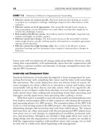
B
A
f
machine
Input
x
(a) A function as a mapping
Output
f(x)
(b) A function as a machine
FIGURE 1.1 Interpretations of the function f(x).
It may help to think of such a function as a “mapping” from numbers in A to numbers in B (Figure 1.1a), or as a “machine” that takes a given number from A and converts it into a number in B through a process indicated by the functional rule (Figure 1.1b).
For instance, the function f(x) ϭ x2 ϩ 4 can be thought of as an “f machine” that accepts
an input x, then squares it and adds 4 to produce an output y ϭ x2 ϩ 4.
No matter how you choose to think of a functional relationship, it is important
to remember that a function assigns one and only one number in the range (output)
to each number in the domain (input). Here is an example.
EXPLORE!
Store f(x) ϭ x2 ϩ 4 into your
graphing utility. Evaluate at
x ϭ Ϫ3, Ϫ1, 0, 1, and 3. Make
a table of values. Repeat
using g(x) ϭ x2 Ϫ 1. Explain
how the values of f(x) and g(x)
differ for each x value.
EXAMPLE 1.1.1
Find f(3) if f(x) ϭ x2 ϩ 4.
Solution
f(3) ϭ 32 ϩ 4 ϭ 13
hof32339_ch01_001-100.qxd 11/17/08 3:02 PM Page 3 User-S198 201:MHDQ082:mhhof10%0:hof10ch01:
1-3
SECTION 1.1 FUNCTIONS
3
Observe the convenience and simplicity of the functional notation. In Example 1.1.1,
the compact formula f(x) ϭ x2 ϩ 4 completely defines the function, and you can indicate
that 13 is the number the function assigns to 3 by simply writing f(3) ϭ 13.
It is often convenient to represent a functional relationship by an equation y ϭ
f(x), and in this context, x and y are called variables. In particular, since the numerical value of y is determined by that of x, we refer to y as the dependent variable
and to x as the independent variable. Note that there is nothing sacred about the
symbols x and y. For example, the function y ϭ x2 ϩ 4 can just as easily be represented by s ϭ t2 ϩ 4 or by w ϭ u2 ϩ 4.
Functional notation can also be used to describe tabular data. For instance,
Table 1.1 lists the average tuition and fees for private 4-year colleges at 5-year intervals from 1973 to 2003.
TABLE 1.1 Average Tuition and Fees for
4-Year Private Colleges
Academic
Year
Ending in
Period n
Tuition and
Fees
1973
1
$1,898
1978
2
$2,700
1983
3
$4,639
1988
4
$7,048
1993
5
$10,448
1998
6
$13,785
2003
7
$18,273
SOURCE: Annual Survey of Colleges, The College Board, New York.
We can describe this data as a function f defined by the rule
f(n) ϭ
Just-In-Time REVIEW
b
Recall that x a/b ϭ ͙x a
whenever a and b are positive
integers. Example 1.1.2 uses
the case when a ؍1 and
b ؍2; x1/2 is another way of
expressing ͙x.
tuition and fees at the
΄average
beginning of the nth 5-year period΅
Thus, f (1) ϭ 1,898, f(2) ϭ 2,700, . . . , f (7) ϭ 18,273. Note that the domain of f is the
set of integers A ϭ {1, 2, . . . , 7}.
The use of functional notation is illustrated further in Examples 1.1.2 and 1.1.3.
In Example 1.1.2, notice that letters other than f and x are used to denote the function and its independent variable.
EXAMPLE 1.1.2
If g(t) ϭ (t Ϫ 2)1/2, find (if possible) g(27), g(5), g(2), and g(1).
Solution
Rewrite the function as g(t) ϭ ͙t Ϫ 2. (If you need to brush up on fractional powers, consult the discussion of exponential notation in Appendix A1. Then
and
g(27) ϭ ͙27 Ϫ 2 ϭ ͙25 ϭ 5
g(5) ϭ ͙5 Ϫ 2 ϭ ͙3 Ϸ 1.7321
g(2) ϭ ͙2 Ϫ 2 ϭ ͙0 ϭ 0
hof32339_ch01_001-100.qxd 11/17/08 3:02 PM Page 4 User-S198 201:MHDQ082:mhhof10%0:hof10ch01:
4
CHAPTER 1 Functions, Graphs, and Limits
EXPLORE!
Store g(x) ͙ ؍x ؊ 2 in the
function editor of your
graphing utility as
Y1 (͙ ؍x ؊ 2). Now on your
HOME SCREEN create
Y1(27), Y1(5), and Y1(2), or,
alternatively, Y1({27, 5, 2}),
where the braces are used to
enclose a list of values. What
happens when you construct
Y1(1)?
However, g(1) is undefined since
g(1) ϭ ͙1 Ϫ 2 ϭ ͙Ϫ1
and negative numbers do not have real square roots.
Functions are often defined using more than one formula, where each individual formula describes the function on a subset of the domain. A function defined in this way is
sometimes called a piecewise-defined function. Here is an example of such a function.
EXAMPLE 1.1.3
12 , f(1), and f(2) if
Find f Ϫ
EXPLORE!
Create a simple piecewisedefined function using the
boolean algebra features of
your graphing utility. Write
Y1 ؍2(X , 1) ؉ (؊1)(X $ 1) in
the function editor. Examine
the graph of this function,
using the ZOOM Decimal
Window. What values does
Y1 assume at X ؍؊2, 0, 1,
and 3?
1-4
Ά
1
f(x) ϭ x Ϫ 1
3x 2 ϩ 1
if x Ͻ 1
if x Ն 1
Solution
1
Since x ϭ Ϫ satisfies x Ͻ 1, use the top part of the formula to find
2
1
1
1
2
f Ϫ ϭ
ϭ
ϭϪ
2
Ϫ1/2 Ϫ 1 Ϫ3/2
3
However, x ϭ 1 and x ϭ 2 satisfy x Ն 1, so f(1) and f (2) are both found by using the
bottom part of the formula:
f(1) ϭ 3(1)2 ϩ 1 ϭ 4
and
f (2) ϭ 3(2)2 ϩ 1 ϭ 13
Domain Convention ■ Unless otherwise specified, if a formula (or several
formulas, as in Example 1.1.3) is used to define a function f, then we assume the
domain of f to be the set of all numbers for which f(x) is defined (as a real number). We refer to this as the natural domain of f.
EXPLORE!
Store f(x) ؍1/(x ؊ 3) in your
graphing utility as Y1, and
display its graph using a
ZOOM Decimal Window.
TRACE values of the function
from X ؍2.5 to 3.5. What do
you notice at X ؍3? Next
store g(x) (͙ ؍x ؊ 2) into Y1,
and graph using a ZOOM
Decimal Window. TRACE
values from X ؍0 to 3, in 0.1
increments. When do the Y
values start to appear, and
what does this tell you about
the domain of g(x)?
Determining the natural domain of a function often amounts to excluding all numbers x that result in dividing by 0 or in taking the square root of a negative number.
This procedure is illustrated in Example 1.1.4.
EXAMPLE 1.1.4
Find the domain and range of each of these functions.
a. f(x) ϭ
1
xϪ3
b.
g(t) ϭ ͙t Ϫ 2
Solution
a. Since division by any number other than 0 is possible, the domain of f is the set
of all numbers x such that x Ϫ 3 ϶ 0; that is, x ϶ 3. The range of f is the set of
1
all numbers y except 0, since for any y ϶ 0, there is an x such that y ϭ
;
xϪ3
1
in particular, x ϭ 3 ϩ .
y
hof32339_ch01_001-100.qxd 11/17/08 3:02 PM Page 5 User-S198 201:MHDQ082:mhhof10%0:hof10ch01:
1-5
SECTION 1.1 FUNCTIONS
Just-In-Time REVIEW
Recall that ͙a is defined to
be the positive number whose
square is a.
Functions Used
in Economics
5
b. Since negative numbers do not have real square roots, g(t) can be evaluated only
when t Ϫ 2 Ն 0, so the domain of g is the set of all numbers t such that t Ն 2.
The range of g is the set of all nonnegative numbers, for if y Ն 0 is any such
number, there is a t such that y ϭ ͙t Ϫ 2; namely, t ϭ y2 ϩ 2.
There are several functions associated with the marketing of a particular commodity:
The demand function D(x) for the commodity is the price p ϭ D(x) that must be
charged for each unit of the commodity if x units are to be sold (demanded).
The supply function S(x) for the commodity is the unit price p ϭ S(x) at which producers are willing to supply x units to the market.
The revenue R(x) obtained from selling x units of the commodity is given by the
product
R(x) ϭ (number of items sold)(price per item)
ϭ xp (x)
The cost function C(x) is the cost of producing x units of the commodity.
The profit function P(x) is the profit obtained from selling x units of the commodity
and is given by the difference
p
P(x) ϭ revenue Ϫ cost
ϭ R(x) Ϫ C(x) ϭ xp(x) Ϫ C(x)
Supply
Demand
x
Generally speaking, the higher the unit price, the fewer the number of units
demanded, and vice versa. Conversely, an increase in unit price leads to an increase in
the number of units supplied. Thus, demand functions are typically decreasing (“falling”
from left to right), while supply functions are increasing (“rising”), as illustrated in the
margin. Here is an example that uses several of these special economic functions.
EXAMPLE 1.1.5
Market research indicates that consumers will buy x thousand units of a particular
kind of coffee maker when the unit price is
p(x) ϭ Ϫ0.27x ϩ 51
dollars. The cost of producing the x thousand units is
C(x) ϭ 2.23x2 ϩ 3.5x ϩ 85
thousand dollars.
a. What are the revenue and profit functions, R(x) and P(x), for this production process?
b. For what values of x is production of the coffee makers profitable?
Just-In-Time REVIEW
Solution
a. The revenue is
The product of two numbers
is positive if they have the
same sign and is negative if
they have different signs. That
is, ab . 0 if a . 0 and b . 0
and also if a , 0 and b , 0.
On the other hand, ab , 0 if
a , 0 and b . 0 or if a . 0
and b , 0.
R(x) ϭ xp(x) ϭ Ϫ0.27x2 ϩ 51x
thousand dollars, and the profit is
P(x) ϭ R(x) Ϫ C(x)
ϭ Ϫ0.27x 2 ϩ 51x Ϫ (2.23x 2 ϩ 3.5x ϩ 85)
ϭ Ϫ2.5x 2 ϩ 47.5x Ϫ 85
thousand dollars.
hof32339_ch01_001-100.qxd 11/17/08 3:02 PM Page 6 User-S198 201:MHDQ082:mhhof10%0:hof10ch01:
6
CHAPTER 1 Functions, Graphs, and Limits
1-6
b. Production is profitable when P(x) Ͼ 0. We find that
P(x) ϭ Ϫ2.5x 2 ϩ 47.5x Ϫ 85
ϭ Ϫ2.5(x 2 Ϫ 19x ϩ 34)
ϭ Ϫ2.5(x Ϫ 2)(x Ϫ 17)
Since the coefficient Ϫ2.5 is negative, it follows that P(x) Ͼ 0 only if the terms
(x Ϫ 2) and (x Ϫ 17) have different signs; that is, when x Ϫ 2 Ͼ 0 and
x Ϫ 17 Ͻ 0. Thus, production is profitable for 2 Ͻ x Ͻ 17.
Example 1.1.6 illustrates how functional notation is used in a practical situation.
Notice that to make the algebraic formula easier to interpret, letters suggesting the
relevant practical quantities are used for the function and its independent variable. (In
this example, the letter C stands for “cost” and q stands for “quantity” manufactured.)
EXPLORE!
Refer to Example 1.1.6, and
store the cost function C(q)
into Y1 as
X3 Ϫ 30X2 ϩ 500X ϩ 200
Construct a TABLE of values
for C(q) using your calculator,
setting TblStart at X ϭ 5 with
an increment ΔTbl ϭ 1 unit.
On the table of values observe
the cost of manufacturing the
10th unit.
EXAMPLE 1.1.6
Suppose the total cost in dollars of manufacturing q units of a certain commodity is
given by the function C(q) ϭ q3 Ϫ 30q2 ϩ 500q ϩ 200.
a. Compute the cost of manufacturing 10 units of the commodity.
b. Compute the cost of manufacturing the 10th unit of the commodity.
Solution
a. The cost of manufacturing 10 units is the value of the total cost function when
q ϭ 10. That is,
Cost of 10 units ϭ C(10)
ϭ (10)3 Ϫ 30(10)2 ϩ 500(10) ϩ 200
ϭ $3,200
b. The cost of manufacturing the 10th unit is the difference between the cost of
manufacturing 10 units and the cost of manufacturing 9 units. That is,
Cost of 10th unit ϭ C(10) Ϫ C(9) ϭ 3,200 Ϫ 2,999 ϭ $201
Composition
of Functions
There are many situations in which a quantity is given as a function of one variable
that, in turn, can be written as a function of a second variable. By combining the
functions in an appropriate way, you can express the original quantity as a function
of the second variable. This process is called composition of functions or functional
composition.
For instance, suppose environmentalists estimate that when p thousand people
live in a certain city, the average daily level of carbon monoxide in the air will be
c(p) parts per million, and that separate demographic studies indicate the population
in t years will be p(t) thousand. What level of pollution should be expected in t years?
You would answer this question by substituting p(t) into the pollution formula c(p)
to express c as a composite function of t.
We shall return to the pollution problem in Example 1.1.11 with specific formulas
for c(p) and p(t), but first you need to see a few examples of how composite functions are formed and evaluated. Here is a definition of functional composition.
hof32339_ch01_001-100.qxd 11/17/08 3:02 PM Page 7 User-S198 201:MHDQ082:mhhof10%0:hof10ch01:
1-7
SECTION 1.1 FUNCTIONS
7
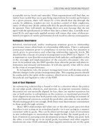
Composition of Functions ■ Given functions f(u) and g(x), the composition f(g(x)) is the function of x formed by substituting u ϭ g(x) for u in the formula for f(u).
Note that the composite function f (g(x)) “makes sense” only if the domain of f
contains the range of g. In Figure 1.2, the definition of composite function is illustrated as an “assembly line” in which “raw” input x is first converted into a transitional product g(x) that acts as input the f machine uses to produce f(g(x)).
g
Output . . .
g
Input
x x x
g
Machine
g(x) g(x)
f
Output
f
Input
g(x) g(x)
f
Machine
f (g(x))
FIGURE 1.2 The composition f (g(x)) as an assembly line.
EXAMPLE 1.1.7
Find the composite function f(g(x)), where f(u) ϭ u2 ϩ 3u ϩ 1 and g(x) ϭ x ϩ 1.
Solution
Replace u by x ϩ 1 in the formula for f (u) to get
EXPLORE!
Store the functions f(x) ϭ x2
and g(x) ϭ x ϩ 3 into Y1 and
Y2, respectively, of the
function editor. Deselect (turn
off) Y1 and Y2. Set Y3 ϭ
Y1(Y2) and Y4 ϭ Y2(Y1). Show
graphically (using ZOOM
Standard) and analytically (by
table values) that f(g(x))
represented by Y3 and g(f(x))
represented by Y4 are not the
same functions. What are the
explicit equations for both of
these composites?
f (g(x)) ϭ (x ϩ 1)2 ϩ 3(x ϩ 1) ϩ 1
ϭ (x2 ϩ 2x ϩ 1) ϩ (3x ϩ 3) ϩ 1
ϭ x2 ϩ 5x ϩ 5
NOTE By reversing the roles of f and g in the definition of composite function, you can define the composition g( f(x)). In general, f (g(x)) and g( f (x)) will
not be the same. For instance, with the functions in Example 1.1.7, you first
write
g(w) ϭ w ϩ 1
and
f(x) ϭ x2 ϩ 3x ϩ 1
and then replace w by x2 ϩ 3x ϩ 1 to get
g( f(x)) ϭ (x2 ϩ 3x ϩ 1) ϩ 1
ϭ x2 ϩ 3x ϩ 2
3
which is equal to f (g(x)) ϭ x2 ϩ 5x ϩ 5 only when x ϭ Ϫ (you should verify
2
this). ■
Example 1.1.7 could have been worded more compactly as follows: Find the composite function f(x ϩ 1) where f(x) ϭ x2 ϩ 3x ϩ 1. The use of this compact notation
is illustrated further in Example 1.1.8.
hof32339_ch01_001-100.qxd 11/17/08 3:02 PM Page 8 User-S198 201:MHDQ082:mhhof10%0:hof10ch01:
8
CHAPTER 1 Functions, Graphs, and Limits
EXPLORE!
Refer to Example 1.1.8. Store
f(x) ؍3x2 ϩ 1/x ϩ 5 into Y1.
Write Y2 ϭ Y1(X Ϫ 1). Construct
a table of values for Y1 and Y2
for 0, 1, . . . , 6. What do you
notice about the values for
Y1 and Y2?
1-8
EXAMPLE 1.1.8
Find f(x Ϫ 1) if f(x) ϭ 3x2 ϩ
1
ϩ 5.
x
Solution
At first glance, this problem may look confusing because the letter x appears both
as the independent variable in the formula defining f and as part of the expression
x Ϫ 1. Because of this, you may find it helpful to begin by writing the formula for
f in more neutral terms, say as
f ( □ ) ϭ 3( □ )2 ϩ
1
ϩ5
□
To find f(x Ϫ 1), you simply insert the expression x Ϫ 1 inside each box, getting
f(x Ϫ 1) ϭ 3(x Ϫ 1)2 ϩ
1
ϩ5
xϪ1
Occasionally, you will have to “take apart” a given composite function g(h(x))
and identify the “outer function” g(u) and “inner function” h(x) from which it was
formed. The procedure is demonstrated in Example 1.1.9.
EXAMPLE 1.1.9
If f(x) ϭ
5
ϩ 4(x Ϫ 2)3, find functions g(u) and h(x) such that f (x) ϭ g(h(x)).
xϪ2
Solution
The form of the given function is
f(x) ϭ
5
ϩ 4( □ )3
□
where each box contains the expression x Ϫ 2. Thus, f (x) ϭ g(h(x)), where
⎞
⎪
⎪
⎬
⎪
⎪
⎠
5
ϩ 4u3
u
and
h(x) ϭ x Ϫ 2
⎞
⎪
⎪
⎬
⎪
⎪
⎠
g(u) ϭ
outer function
inner function
Actually, in Example 1.1.9, there are infinitely many pairs of functions g(u)
5
and h(x) that combine to give g(h(x)) ϭ f(x). [For example, g(u) ϭ
ϩ 4(u ϩ 1)3
uϩ1
and h(x) ϭ x Ϫ 3.] The particular pair selected in the solution to this example is the
most natural one and reflects most clearly the structure of the original function f(x).
EXAMPLE 1.1.10
A difference quotient is an expression of the general form
f(x ϩ h) Ϫ f(x)
h