Ebook Data structures and algorithm analysis in C++ (4th edition) Part 2
Bạn đang xem bản rút gọn của tài liệu. Xem và tải ngay bản đầy đủ của tài liệu tại đây (4.18 MB, 345 trang )
C H A P T E R
7
Sorting
In this chapter, we discuss the problem of sorting an array of elements. To simplify matters,
we will assume in our examples that the array contains only integers, although our code
will once again allow more general objects. For most of this chapter, we will also assume
that the entire sort can be done in main memory, so that the number of elements is relatively
small (less than a few million). Sorts that cannot be performed in main memory and must
be done on disk or tape are also quite important. This type of sorting, known as external
sorting, will be discussed at the end of the chapter.
Our investigation of internal sorting will show that. . .
r
There are several easy algorithms to sort in O(N2 ), such as insertion sort.
r
There is an algorithm, Shellsort, that is very simple to code, runs in o(N2 ), and is
efficient in practice.
r There are slightly more complicated O(N log N) sorting algorithms.
r
Any general-purpose sorting algorithm requires
(N log N) comparisons.
The rest of this chapter will describe and analyze the various sorting algorithms. These
algorithms contain interesting and important ideas for code optimization as well as algorithm design. Sorting is also an example where the analysis can be precisely performed. Be
forewarned that where appropriate, we will do as much analysis as possible.
7.1 Preliminaries
The algorithms we describe will all be interchangeable. Each will be passed an array containing the elements; we assume all array positions contain data to be sorted. We will
assume that N is the number of elements passed to our sorting routines.
We will also assume the existence of the “<” and “>” operators, which can be used
to place a consistent ordering on the input. Besides the assignment operator, these are the
only operations allowed on the input data. Sorting under these conditions is known as
comparison-based sorting.
This interface is not the same as in the STL sorting algorithms. In the STL, sorting is
accomplished by use of the function template sort. The parameters to sort represent the
start and endmarker of a (range in a) container and an optional comparator:
void sort( Iterator begin, Iterator end );
void sort( Iterator begin, Iterator end, Comparator cmp );
291
292
Chapter 7
Sorting
The iterators must support random access. The sort algorithm does not guarantee that
equal items retain their original order (if that is important, use stable_sort instead of sort).
As an example, in
std::sort( v.begin( ), v.end( ) );
std::sort( v.begin( ), v.end( ), greater<int>{ } );
std::sort( v.begin( ), v.begin( ) + ( v.end( ) - v.begin( ) ) / 2 );
the first call sorts the entire container, v, in nondecreasing order. The second call sorts the
entire container in nonincreasing order. The third call sorts the first half of the container
in nondecreasing order.
The sorting algorithm used is generally quicksort, which we describe in Section 7.7.
In Section 7.2, we implement the simplest sorting algorithm using both our style of passing the array of comparable items, which yields the most straightforward code, and the
interface supported by the STL, which requires more code.
7.2 Insertion Sort
One of the simplest sorting algorithms is the insertion sort.
7.2.1 The Algorithm
Insertion sort consists of N − 1 passes. For pass p = 1 through N − 1, insertion sort ensures
that the elements in positions 0 through p are in sorted order. Insertion sort makes use of
the fact that elements in positions 0 through p − 1 are already known to be in sorted order.
Figure 7.1 shows a sample array after each pass of insertion sort.
Figure 7.1 shows the general strategy. In pass p, we move the element in position p left
until its correct place is found among the first p+1 elements. The code in Figure 7.2 implements this strategy. Lines 11 to 14 implement that data movement without the explicit use
of swaps. The element in position p is moved to tmp, and all larger elements (prior to position p) are moved one spot to the right. Then tmp is moved to the correct spot. This is the
same technique that was used in the implementation of binary heaps.
Original
34
8
64
51
32
21
Positions Moved
After p = 1
After p = 2
After p = 3
After p = 4
After p = 5
8
8
8
8
8
34
34
34
32
21
64
64
51
34
32
51
51
64
51
34
32
32
32
64
51
21
21
21
21
64
1
0
1
3
4
Figure 7.1 Insertion sort after each pass
7.2 Insertion Sort
1
2
3
4
5
6
7
8
9
10
11
12
13
14
15
16
/**
* Simple insertion sort.
*/
template <typename Comparable>
void insertionSort( vector<Comparable> & a )
{
for( int p = 1; p < a.size( ); ++p )
{
Comparable tmp = std::move( a[ p ] );
int j;
for( j = p; j > 0 && tmp < a[ j - 1 ]; --j )
a[ j ] = std::move( a[ j - 1 ] );
a[ j ] = std::move( tmp );
}
}
Figure 7.2 Insertion sort routine
7.2.2 STL Implementation of Insertion Sort
In the STL, instead of having the sort routines take an array of comparable items as a single
parameter, the sort routines receive a pair of iterators that represent the start and endmarker
of a range. A two-parameter sort routine uses just that pair of iterators and presumes that
the items can be ordered, while a three-parameter sort routine has a function object as a
third parameter.
Converting the algorithm in Figure 7.2 to use the STL introduces several issues. The
obvious issues are
1. We must write a two-parameter sort and a three-parameter sort. Presumably, the twoparameter sort invokes the three-parameter sort, with less<Object>{ } as the third
parameter.
2. Array access must be converted to iterator access.
3. Line 11 of the original code requires that we create tmp, which in the new code will
have type Object.
The first issue is the trickiest because the template type parameters (i.e., the generic
types) for the two-parameter sort are both Iterator; however, Object is not one of the
generic type parameters. Prior to C++11, one had to write extra routines to solve this
problem. As shown in Figure 7.3, C++11 introduces decltype which cleanly expresses the
intent.
Figure 7.4 shows the main sorting code that replaces array indexing with use of the
iterator, and that replaces calls to operator< with calls to the lessThan function object.
Observe that once we actually code the insertionSort algorithm, every statement in
the original code is replaced with a corresponding statement in the new code that makes
293
294
Chapter 7
1
2
3
4
5
6
7
8
9
Sorting
/*
* The two-parameter version calls the three-parameter version,
* using C++11 decltype
*/
template <typename Iterator>
void insertionSort( const Iterator & begin, const Iterator & end )
{
insertionSort( begin, end, less<decltype(*begin)>{ } );
}
Figure 7.3 Two-parameter sort invokes three-parameter sort via C++11 decltype
1
2
3
4
5
6
7
8
9
10
11
12
13
14
15
16
17
template <typename Iterator, typename Comparator>
void insertionSort( const Iterator & begin, const Iterator & end,
Comparator lessThan )
{
if( begin == end )
return;
Iterator j;
for( Iterator p = begin+1; p != end; ++p )
{
auto tmp = std::move( *p );
for( j = p; j != begin && lessThan( tmp, *( j-1 ) ); --j )
*j = std::move( *(j-1) );
*j = std::move( tmp );
}
}
Figure 7.4 Three-parameter sort using iterators
straightforward use of iterators and the function object. The original code is arguably much
simpler to read, which is why we use our simpler interface rather than the STL interface
when coding our sorting algorithms.
7.2.3 Analysis of Insertion Sort
Because of the nested loops, each of which can take N iterations, insertion sort is O(N2 ).
Furthermore, this bound is tight, because input in reverse order can achieve this bound.
A precise calculation shows that the number of tests in the inner loop in Figure 7.2 is at
most p + 1 for each value of p. Summing over all p gives a total of
N
i = 2 + 3 + 4 + ··· + N =
i=2
(N2 )
7.3 A Lower Bound for Simple Sorting Algorithms
On the other hand, if the input is presorted, the running time is O(N), because the
test in the inner for loop always fails immediately. Indeed, if the input is almost sorted
(this term will be more rigorously defined in the next section), insertion sort will run
quickly. Because of this wide variation, it is worth analyzing the average-case behavior of
this algorithm. It turns out that the average case is (N2 ) for insertion sort, as well as for
a variety of other sorting algorithms, as the next section shows.
7.3 A Lower Bound for Simple
Sorting Algorithms
An inversion in an array of numbers is any ordered pair (i, j) having the property that i < j
but a[i] > a[j]. In the example of the last section, the input list 34, 8, 64, 51, 32, 21 had
nine inversions, namely (34, 8), (34, 32), (34, 21), (64, 51), (64, 32), (64, 21), (51, 32),
(51, 21), and (32, 21). Notice that this is exactly the number of swaps that needed to be
(implicitly) performed by insertion sort. This is always the case, because swapping two
adjacent elements that are out of place removes exactly one inversion, and a sorted array
has no inversions. Since there is O(N) other work involved in the algorithm, the running
time of insertion sort is O(I + N), where I is the number of inversions in the original array.
Thus, insertion sort runs in linear time if the number of inversions is O(N).
We can compute precise bounds on the average running time of insertion sort by
computing the average number of inversions in a permutation. As usual, defining average is a difficult proposition. We will assume that there are no duplicate elements (if we
allow duplicates, it is not even clear what the average number of duplicates is). Using this
assumption, we can assume that the input is some permutation of the first N integers (since
only relative ordering is important) and that all are equally likely. Under these assumptions,
we have the following theorem:
Theorem 7.1
The average number of inversions in an array of N distinct elements is N(N − 1)/4.
Proof
For any list, L, of elements, consider Lr , the list in reverse order. The reverse list of the
example is 21, 32, 51, 64, 8, 34. Consider any pair of two elements in the list (x, y) with
y > x. Clearly, in exactly one of L and Lr this ordered pair represents an inversion. The
total number of these pairs in a list L and its reverse Lr is N(N − 1)/2. Thus, an average
list has half this amount, or N(N − 1)/4 inversions.
This theorem implies that insertion sort is quadratic on average. It also provides a very
strong lower bound about any algorithm that only exchanges adjacent elements.
Theorem 7.2
Any algorithm that sorts by exchanging adjacent elements requires
average.
(N2 ) time on
295
296
Chapter 7
Sorting
Proof
The average number of inversions is initially N(N−1)/4 =
only one inversion, so (N2 ) swaps are required.
(N2 ). Each swap removes
This is an example of a lower-bound proof. It is valid not only for insertion sort, which
performs adjacent exchanges implicitly, but also for other simple algorithms such as bubble
sort and selection sort, which we will not describe here. In fact, it is valid over an entire class
of sorting algorithms, including those undiscovered, that perform only adjacent exchanges.
Because of this, this proof cannot be confirmed empirically. Although this lower-bound
proof is rather simple, in general proving lower bounds is much more complicated than
proving upper bounds and in some cases resembles magic.
This lower bound shows us that in order for a sorting algorithm to run in subquadratic,
or o(N2 ), time, it must do comparisons and, in particular, exchanges between elements
that are far apart. A sorting algorithm makes progress by eliminating inversions, and to run
efficiently, it must eliminate more than just one inversion per exchange.
7.4 Shellsort
Shellsort, named after its inventor, Donald Shell, was one of the first algorithms to break
the quadratic time barrier, although it was not until several years after its initial discovery
that a subquadratic time bound was proven. As suggested in the previous section, it works
by comparing elements that are distant; the distance between comparisons decreases as
the algorithm runs until the last phase, in which adjacent elements are compared. For this
reason, Shellsort is sometimes referred to as diminishing increment sort.
Shellsort uses a sequence, h1 , h2 , . . . , ht , called the increment sequence. Any increment sequence will do as long as h1 = 1, but some choices are better than others (we
will discuss that issue later). After a phase, using some increment hk , for every i, we have
a[i] ≤ a[i + hk ] (where this makes sense); all elements spaced hk apart are sorted. The file
is then said to be hk -sorted. For example, Figure 7.5 shows an array after several phases
of Shellsort. An important property of Shellsort (which we state without proof) is that an
hk -sorted file that is then hk−1 -sorted remains hk -sorted. If this were not the case, the algorithm would likely be of little value, since work done by early phases would be undone by
later phases.
The general strategy to hk -sort is for each position, i, in hk , hk + 1, . . . , N − 1, place
the element in the correct spot among i, i − hk , i − 2hk , and so on. Although this does not
Original
81
94
11
96
12
35
17
95
28
58
41
75
15
After 5-sort
After 3-sort
After 1-sort
35
28
11
17
12
12
11
11
15
28
35
17
12
15
28
41
41
35
75
58
41
15
17
58
96
94
75
58
75
81
81
81
94
94
96
95
95
95
96
Figure 7.5 Shellsort after each pass
7.4 Shellsort
1
2
3
4
5
6
7
8
9
10
11
12
13
14
15
16
17
/**
* Shellsort, using Shell’s (poor) increments.
*/
template <typename Comparable>
void shellsort( vector<Comparable> & a )
{
for( int gap = a.size( ) / 2; gap > 0; gap /= 2 )
for( int i = gap; i < a.size( ); ++i )
{
Comparable tmp = std::move( a[ i ] );
int j = i;
for( ; j >= gap && tmp < a[ j - gap ]; j -= gap )
a[ j ] = std::move( a[ j - gap ] );
a[ j ] = std::move( tmp );
}
}
Figure 7.6 Shellsort routine using Shell’s increments (better increments are possible)
affect the implementation, a careful examination shows that the action of an hk -sort is to
perform an insertion sort on hk independent subarrays. This observation will be important
when we analyze the running time of Shellsort.
A popular (but poor) choice for increment sequence is to use the sequence suggested
by Shell: ht = N/2 , and hk = hk+1 /2 . Figure 7.6 contains a function that implements
Shellsort using this sequence. We shall see later that there are increment sequences that
give a significant improvement in the algorithm’s running time; even a minor change can
drastically affect performance (Exercise 7.10).
The program in Figure 7.6 avoids the explicit use of swaps in the same manner as our
implementation of insertion sort.
7.4.1 Worst-Case Analysis of Shellsort
Although Shellsort is simple to code, the analysis of its running time is quite another
story. The running time of Shellsort depends on the choice of increment sequence, and the
proofs can be rather involved. The average-case analysis of Shellsort is a long-standing open
problem, except for the most trivial increment sequences. We will prove tight worst-case
bounds for two particular increment sequences.
Theorem 7.3
The worst-case running time of Shellsort using Shell’s increments is
(N2 ).
Proof
The proof requires showing not only an upper bound on the worst-case running time
but also showing that there exists some input that actually takes (N2 ) time to run.
297
298
Chapter 7
Sorting
We prove the lower bound first by constructing a bad case. First, we choose N to be a
power of 2. This makes all the increments even, except for the last increment, which
is 1. Now, we will give as input an array with the N/2 largest numbers in the even
positions and the N/2 smallest numbers in the odd positions (for this proof, the first
position is position 1). As all the increments except the last are even, when we come
to the last pass, the N/2 largest numbers are still all in even positions and the N/2
smallest numbers are still all in odd positions. The ith smallest number (i ≤ N/2) is
thus in position 2i − 1 before the beginning of the last pass. Restoring the ith element
to its correct place requires moving it i−1 spaces in the array. Thus, to merely place the
N/2
N/2 smallest elements in the correct place requires at least i=1 i − 1 = (N2 ) work.
As an example, Figure 7.7 shows a bad (but not the worst) input when N = 16. The
number of inversions remaining after the 2-sort is exactly 1+2+3+4+5+6+7 = 28;
thus, the last pass will take considerable time.
To finish the proof, we show the upper bound of O(N2 ). As we have observed
before, a pass with increment hk consists of hk insertion sorts of about N/hk elements.
Since insertion sort is quadratic, the total cost of a pass is O(hk (N/hk )2 ) = O(N2 /hk ).
Summing over all passes gives a total bound of O( ti=1 N2 /hi ) = O(N2 ti=1 1/hi ).
Because the increments form a geometric series with common ratio 2, and the largest
term in the series is h1 = 1, ti=1 1/hi < 2. Thus we obtain a total bound of O(N2 ).
The problem with Shell’s increments is that pairs of increments are not necessarily relatively prime, and thus the smaller increment can have little effect. Hibbard suggested a
slightly different increment sequence, which gives better results in practice (and theoretically). His increments are of the form 1, 3, 7, . . . , 2k − 1. Although these increments are
almost identical, the key difference is that consecutive increments have no common factors. We now analyze the worst-case running time of Shellsort for this increment sequence.
The proof is rather complicated.
Theorem 7.4
The worst-case running time of Shellsort using Hibbard’s increments is
(N3/2 ).
Proof
We will prove only the upper bound and leave the proof of the lower bound as an
exercise. The proof requires some well-known results from additive number theory.
References to these results are provided at the end of the chapter.
For the upper bound, as before, we bound the running time of each pass and sum
over all passes. For increments hk > N1/2 , we will use the bound O(N2 /hk ) from the
Start
1
9
2
10
3
11
4
12
5
13
6
14
7
15
8
16
After 8-sort
After 4-sort
After 2-sort
After 1-sort
1
1
1
1
9
9
9
2
2
2
2
3
10
10
10
4
3
3
3
5
11
11
11
6
4
4
4
7
12
12
12
8
5
5
5
9
13
13
13
10
6
6
6
11
14
14
14
12
7
7
7
13
15
15
15
14
8
8
8
15
16
16
16
16
Figure 7.7 Bad case for Shellsort with Shell’s increments (positions are numbered 1 to 16)
7.4 Shellsort
previous theorem. Although this bound holds for the other increments, it is too large to
be useful. Intuitively, we must take advantage of the fact that this increment sequence
is special. What we need to show is that for any element a[p] in position p, when it is
time to perform an hk -sort, there are only a few elements to the left of position p that
are larger than a[p].
When we come to hk -sort the input array, we know that it has already been hk+1 and hk+2 -sorted. Prior to the hk -sort, consider elements in positions p and p − i, i ≤ p.
If i is a multiple of hk+1 or hk+2 , then clearly a[p − i] < a[p]. We can say more,
however. If i is expressible as a linear combination (in nonnegative integers) of hk+1
and hk+2 , then a[p − i] < a[p]. As an example, when we come to 3-sort, the file
is already 7- and 15-sorted. 52 is expressible as a linear combination of 7 and 15,
because 52 = 1 ∗ 7 + 3 ∗ 15. Thus, a[100] cannot be larger than a[152] because
a[100] ≤ a[107] ≤ a[122] ≤ a[137] ≤ a[152].
Now, hk+2 = 2hk+1 + 1, so hk+1 and hk+2 cannot share a common factor.
In this case, it is possible to show that all integers that are at least as large as
(hk+1 − 1)(hk+2 − 1) = 8h2k + 4hk can be expressed as a linear combination of
hk+1 and hk+2 (see the reference at the end of the chapter).
This tells us that the body of the innermost for loop can be executed at most
8hk + 4 = O(hk ) times for each of the N − hk positions. This gives a bound of O(Nhk )
per pass.
√
Using the fact that about half the increments satisfy hk < N, and assuming that t
is even, the total running time is then
⎛
⎞
⎛
⎞
O⎝
t/2
t
Nhk +
k=1
N2 /hk ⎠ = O ⎝N
k=t/2+1
t/2
t
hk + N 2
k=1
Because both sums are geometric series, and since ht/2 =
= O Nht/2 + O
N2
ht/2
1/hk ⎠
k=t/2+1
√
( N), this simplifies to
= O(N3/2 )
The average-case running time of Shellsort, using Hibbard’s increments, is thought to
be O(N5/4 ), based on simulations, but nobody has been able to prove this. Pratt has shown
that the (N3/2 ) bound applies to a wide range of increment sequences.
Sedgewick has proposed several increment sequences that give an O(N4/3 ) worstcase running time (also achievable). The average running time is conjectured to be
O(N7/6 ) for these increment sequences. Empirical studies show that these sequences perform significantly better in practice than Hibbard’s. The best of these is the sequence
{1, 5, 19, 41, 109, . . .}, in which the terms are either of the form 9 · 4i − 9 · 2i + 1 or
4i − 3 · 2i + 1. This is most easily implemented by placing these values in an array. This
increment sequence is the best known in practice, although there is a lingering possibility
that some increment sequence might exist that could give a significant improvement in the
running time of Shellsort.
There are several other results on Shellsort that (generally) require difficult theorems
from number theory and combinatorics and are mainly of theoretical interest. Shellsort is
a fine example of a very simple algorithm with an extremely complex analysis.
299
300
Chapter 7
Sorting
The performance of Shellsort is quite acceptable in practice, even for N in the tens of
thousands. The simplicity of the code makes it the algorithm of choice for sorting up to
moderately large input.
7.5 Heapsort
As mentioned in Chapter 6, priority queues can be used to sort in O(N log N) time. The
algorithm based on this idea is known as heapsort and gives the best Big-Oh running time
we have seen so far.
Recall from Chapter 6 that the basic strategy is to build a binary heap of N elements.
This stage takes O(N) time. We then perform N deleteMin operations. The elements leave
the heap smallest first, in sorted order. By recording these elements in a second array and
then copying the array back, we sort N elements. Since each deleteMin takes O(log N) time,
the total running time is O(N log N).
The main problem with this algorithm is that it uses an extra array. Thus, the memory
requirement is doubled. This could be a problem in some instances. Notice that the extra
time spent copying the second array back to the first is only O(N), so that this is not likely
to affect the running time significantly. The problem is space.
A clever way to avoid using a second array makes use of the fact that after each
deleteMin, the heap shrinks by 1. Thus the cell that was last in the heap can be used
to store the element that was just deleted. As an example, suppose we have a heap with six
elements. The first deleteMin produces a1 . Now the heap has only five elements, so we can
place a1 in position 6. The next deleteMin produces a2 . Since the heap will now only have
four elements, we can place a2 in position 5.
Using this strategy, after the last deleteMin the array will contain the elements in decreasing sorted order. If we want the elements in the more typical increasing sorted order, we can
change the ordering property so that the parent has a larger element than the child. Thus,
we have a (max)heap.
In our implementation, we will use a (max)heap but avoid the actual ADT for the
purposes of speed. As usual, everything is done in an array. The first step builds the
heap in linear time. We then perform N − 1 deleteMaxes by swapping the last element
in the heap with the first, decrementing the heap size, and percolating down. When
the algorithm terminates, the array contains the elements in sorted order. For instance,
consider the input sequence 31, 41, 59, 26, 53, 58, 97. The resulting heap is shown in
Figure 7.8.
Figure 7.9 shows the heap that results after the first deleteMax. As the figures imply,
the last element in the heap is 31; 97 has been placed in a part of the heap array that is
technically no longer part of the heap. After 5 more deleteMax operations, the heap will
actually have only one element, but the elements left in the heap array will be in sorted
order.
The code to perform heapsort is given in Figure 7.10. The slight complication is that,
unlike the binary heap, where the data begin at array index 1, the array for heapsort contains data in position 0. Thus the code is a little different from the binary heap code. The
changes are minor.
7.5 Heapsort
97
53
59
26
41
58
31
97 53 59 26 41 58 31
0
1
2
3
4
5
6
7
8
9
10
Figure 7.8 (Max) heap after buildHeap phase
59
53
58
26
41
31
97
59 53 58 26 41 31 97
0
1
2
3
4
5
6
7
8
9
10
Figure 7.9 Heap after first deleteMax
7.5.1 Analysis of Heapsort
As we saw in Chapter 6, the first phase, which constitutes the building of the heap, uses
less than 2N comparisons. In the second phase, the ith deleteMax uses at most less than
2 log (N − i + 1) comparisons, for a total of at most 2N log N − O(N) comparisons
(assuming N ≥ 2). Consequently, in the worst case, at most 2N log N − O(N) comparisons are used by heapsort. Exercise 7.13 asks you to show that it is possible for all of the
deleteMax operations to achieve their worst case simultaneously.
301
1
2
3
4
5
6
7
8
9
10
11
12
13
14
15
16
17
18
19
20
21
22
23
24
25
26
27
28
29
30
31
32
33
34
35
36
37
38
39
40
41
42
43
44
45
46
47
48
/**
* Standard heapsort.
*/
template <typename Comparable>
void heapsort( vector<Comparable> & a )
{
for( int i = a.size( ) / 2 - 1; i >= 0; --i ) /* buildHeap */
percDown( a, i, a.size( ) );
for( int j = a.size( ) - 1; j > 0; --j )
{
std::swap( a[ 0 ], a[ j ] );
/* deleteMax */
percDown( a, 0, j );
}
}
/**
* Internal method for heapsort.
* i is the index of an item in the heap.
* Returns the index of the left child.
*/
inline int leftChild( int i )
{
return 2 * i + 1;
}
/**
* Internal method for heapsort that is used in deleteMax and buildHeap.
* i is the position from which to percolate down.
* n is the logical size of the binary heap.
*/
template <typename Comparable>
void percDown( vector<Comparable> & a, int i, int n )
{
int child;
Comparable tmp;
for( tmp = std::move( a[ i ] ); leftChild( i ) < n; i = child )
{
child = leftChild( i );
if( child != n - 1 && a[ child ] < a[ child + 1 ] )
++child;
if( tmp < a[ child ] )
a[ i ] = std::move( a[ child ] );
else
break;
}
a[ i ] = std::move( tmp );
}
Figure 7.10 Heapsort
7.5 Heapsort
Experiments have shown that the performance of heapsort is extremely consistent:
On average it uses only slightly fewer comparisons than the worst-case bound suggests.
For many years, nobody had been able to show nontrivial bounds on heapsort’s average
running time. The problem, it seems, is that successive deleteMax operations destroy the
heap’s randomness, making the probability arguments very complex. Eventually, another
approach proved successful.
Theorem 7.5
The average number of comparisons used to heapsort a random permutation of N
distinct items is 2N log N − O(N log log N).
Proof
The heap construction phase uses (N) comparisons on average, and so we only need
to prove the bound for the second phase. We assume a permutation of {1, 2, . . . , N}.
Suppose the ith deleteMax pushes the root element down di levels. Then it uses 2di
comparisons. For heapsort on any input, there is a cost sequence D : d1 , d2 , . . . , dN
that defines the cost of phase 2. That cost is given by MD = N
i=1 di ; the number of
comparisons used is thus 2MD .
Let f(N) be the number of heaps of N items. One can show (Exercise 7.58) that
f(N) > (N/(4e))N (where e = 2.71828 . . .). We will show that only an exponentially
small fraction of these heaps (in particular (N/16)N ) have a cost smaller than M =
N(log N − log log N − 4). When this is shown, it follows that the average value of MD
is at least M minus a term that is o(1), and thus the average number of comparisons is
at least 2M. Consequently, our basic goal is to show that there are very few heaps that
have small cost sequences.
Because level di has at most 2di nodes, there are 2di possible places that the root
element can go for any di . Consequently, for any sequence D, the number of distinct
corresponding deleteMax sequences is at most
SD = 2d1 2d2 · · · 2dN
A simple algebraic manipulation shows that for a given sequence D,
S D = 2 MD
Because each di can assume any value between 1 and log N , there are at
most (log N)N possible sequences D. It follows that the number of distinct deleteMax
sequences that require cost exactly equal to M is at most the number of cost sequences
of total cost M times the number of deleteMax sequences for each of these cost
sequences. A bound of (log N)N 2M follows immediately.
The total number of heaps with cost sequence less than M is at most
M−1
(log N)N 2i < (log N)N 2M
i=1
303
304
Chapter 7
Sorting
If we choose M = N(log N − log log N − 4), then the number of heaps that have
cost sequence less than M is at most (N/16)N , and the theorem follows from our earlier
comments.
Using a more complex argument, it can be shown that heapsort always uses at least
N log N − O(N) comparisons and that there are inputs that can achieve this bound. The
average-case analysis also can be improved to 2N log N − O(N) comparisons (rather than
the nonlinear second term in Theorem 7.5).
7.6 Mergesort
We now turn our attention to mergesort. Mergesort runs in O(N log N) worst-case running
time, and the number of comparisons used is nearly optimal. It is a fine example of a
recursive algorithm.
The fundamental operation in this algorithm is merging two sorted lists. Because the
lists are sorted, this can be done in one pass through the input, if the output is put in a
third list. The basic merging algorithm takes two input arrays A and B, an output array C,
and three counters, Actr, Bctr, and Cctr, which are initially set to the beginning of their
respective arrays. The smaller of A[Actr] and B[Bctr] is copied to the next entry in C, and
the appropriate counters are advanced. When either input list is exhausted, the remainder
of the other list is copied to C. An example of how the merge routine works is provided for
the following input.
1
13
24
26
↑
Actr
2
15
27
38
↑
Bctr
↑
Cctr
If the array A contains 1, 13, 24, 26, and B contains 2, 15, 27, 38, then the algorithm
proceeds as follows: First, a comparison is done between 1 and 2. 1 is added to C, and
then 13 and 2 are compared.
1
13
24
26
↑
Actr
2
15
27
38
1
↑
Bctr
↑
Cctr
2 is added to C, and then 13 and 15 are compared.
1
13
↑
Actr
24
26
2
15
↑
Bctr
27
38
1
2
↑
Cctr
7.6 Mergesort
13 is added to C, and then 24 and 15 are compared. This proceeds until 26 and 27 are
compared.
1
13
24
26
2
↑
Actr
1
13
24
15
26
2
15
↑
Actr
1
13
24
27
38
1
2
13
↑
Bctr
↑
Cctr
27
38
1
2
13
15
↑
Bctr
26
2
15
↑
Actr
27
↑
Cctr
38
1
2
13
15
24
↑
Bctr
↑
Cctr
26 is added to C, and the A array is exhausted.
1
13
24
26
2
15
↑
Actr
27
38
1
2
13
15
24
26
↑
Bctr
↑
Cctr
The remainder of the B array is then copied to C.
1
13
24
26
2
↑
Actr
15
27
38
1
↑
Bctr
2
13
15
24
26
27
38
↑
Cctr
The time to merge two sorted lists is clearly linear, because at most N − 1 comparisons
are made, where N is the total number of elements. To see this, note that every comparison
adds an element to C, except the last comparison, which adds at least two.
The mergesort algorithm is therefore easy to describe. If N = 1, there is only one
element to sort, and the answer is at hand. Otherwise, recursively mergesort the first half
and the second half. This gives two sorted halves, which can then be merged together
using the merging algorithm described above. For instance, to sort the eight-element array
24, 13, 26, 1, 2, 27, 38, 15, we recursively sort the first four and last four elements, obtaining 1, 13, 24, 26, 2, 15, 27, 38. Then we merge the two halves as above, obtaining the final
list 1, 2, 13, 15, 24, 26, 27, 38. This algorithm is a classic divide-and-conquer strategy. The
problem is divided into smaller problems and solved recursively. The conquering phase
consists of patching together the answers. Divide-and-conquer is a very powerful use of
recursion that we will see many times.
An implementation of mergesort is provided in Figure 7.11. The one-parameter
mergeSort is just a driver for the four-parameter recursive mergeSort.
The merge routine is subtle. If a temporary array is declared locally for each recursive
call of merge, then there could be log N temporary arrays active at any point. A close examination shows that since merge is the last line of mergeSort, there only needs to be one
305
306
Chapter 7
1
2
3
4
5
6
7
8
9
10
11
12
13
14
15
16
17
18
19
20
21
22
23
24
25
26
27
28
29
30
Sorting
/**
* Mergesort algorithm (driver).
*/
template <typename Comparable>
void mergeSort( vector<Comparable> & a )
{
vector<Comparable> tmpArray( a.size( ) );
mergeSort( a, tmpArray, 0, a.size( ) - 1 );
}
/**
* Internal method that makes recursive calls.
* a is an array of Comparable items.
* tmpArray is an array to place the merged result.
* left is the left-most index of the subarray.
* right is the right-most index of the subarray.
*/
template <typename Comparable>
void mergeSort( vector<Comparable> & a,
vector<Comparable> & tmpArray, int left, int right )
{
if( left < right )
{
int center = ( left + right ) / 2;
mergeSort( a, tmpArray, left, center );
mergeSort( a, tmpArray, center + 1, right );
merge( a, tmpArray, left, center + 1, right );
}
}
Figure 7.11 Mergesort routines
temporary array active at any point, and that the temporary array can be created in the
public mergeSort driver. Further, we can use any part of the temporary array; we will use
the same portion as the input array a. This allows the improvement described at the end of
this section. Figure 7.12 implements the merge routine.
7.6.1 Analysis of Mergesort
Mergesort is a classic example of the techniques used to analyze recursive routines: We
have to write a recurrence relation for the running time. We will assume that N is a power
of 2 so that we always split into even halves. For N = 1, the time to mergesort is constant,
which we will denote by 1. Otherwise, the time to mergesort N numbers is equal to the
7.6 Mergesort
1
2
3
4
5
6
7
8
9
10
11
12
13
14
15
16
17
18
19
20
21
22
23
24
25
26
27
28
29
30
31
32
33
/**
* Internal method that merges two sorted halves of a subarray.
* a is an array of Comparable items.
* tmpArray is an array to place the merged result.
* leftPos is the left-most index of the subarray.
* rightPos is the index of the start of the second half.
* rightEnd is the right-most index of the subarray.
*/
template <typename Comparable>
void merge( vector<Comparable> & a, vector<Comparable> & tmpArray,
int leftPos, int rightPos, int rightEnd )
{
int leftEnd = rightPos - 1;
int tmpPos = leftPos;
int numElements = rightEnd - leftPos + 1;
// Main loop
while( leftPos <= leftEnd && rightPos <= rightEnd )
if( a[ leftPos ] <= a[ rightPos ] )
tmpArray[ tmpPos++ ] = std::move( a[ leftPos++ ] );
else
tmpArray[ tmpPos++ ] = std::move( a[ rightPos++ ] );
while( leftPos <= leftEnd )
// Copy rest of first half
tmpArray[ tmpPos++ ] = std::move( a[ leftPos++ ] );
while( rightPos <= rightEnd ) // Copy rest of right half
tmpArray[ tmpPos++ ] = std::move( a[ rightPos++ ] );
// Copy tmpArray back
for( int i = 0; i < numElements; ++i, --rightEnd )
a[ rightEnd ] = std::move( tmpArray[ rightEnd ] );
}
Figure 7.12 merge routine
time to do two recursive mergesorts of size N/2, plus the time to merge, which is linear.
The following equations say this exactly:
T(1) = 1
T(N) = 2T(N/2) + N
This is a standard recurrence relation, which can be solved several ways. We will show two
methods. The first idea is to divide the recurrence relation through by N. The reason for
doing this will become apparent soon. This yields
307
308
Chapter 7
Sorting
T(N/2)
T(N)
=
+1
N
N/2
This equation is valid for any N that is a power of 2, so we may also write
T(N/2)
T(N/4)
=
+1
N/2
N/4
and
T(N/4)
T(N/8)
=
+1
N/4
N/8
..
.
T(1)
T(2)
=
+1
2
1
Now add up all the equations. This means that we add all of the terms on the left-hand side
and set the result equal to the sum of all of the terms on the right-hand side. Observe that
the term T(N/2)/(N/2) appears on both sides and thus cancels. In fact, virtually all the
terms appear on both sides and cancel. This is called telescoping a sum. After everything
is added, the final result is
T(1)
T(N)
=
+ log N
N
1
because all of the other terms cancel and there are log N equations, and so all the 1s at the
end of these equations add up to log N. Multiplying through by N gives the final answer.
T(N) = N log N + N = O(N log N)
Notice that if we did not divide through by N at the start of the solutions, the sum
would not telescope. This is why it was necessary to divide through by N.
An alternative method is to substitute the recurrence relation continually on the righthand side. We have
T(N) = 2T(N/2) + N
Since we can substitute N/2 into the main equation,
2T(N/2) = 2(2(T(N/4)) + N/2) = 4T(N/4) + N
we have
T(N) = 4T(N/4) + 2N
Again, by substituting N/4 into the main equation, we see that
4T(N/4) = 4(2T(N/8) + N/4) = 8T(N/8) + N
So we have
T(N) = 8T(N/8) + 3N
7.7 Quicksort
Continuing in this manner, we obtain
T(N) = 2k T(N/2k ) + k · N
Using k = log N, we obtain
T(N) = NT(1) + N log N = N log N + N
The choice of which method to use is a matter of taste. The first method tends to
produce scrap work that fits better on a standard 81/2 × 11 sheet of paper leading to fewer
mathematical errors, but it requires a certain amount of experience to apply. The second
method is more of a brute-force approach.
Recall that we have assumed N = 2k . The analysis can be refined to handle cases when
N is not a power of 2. The answer turns out to be almost identical (this is usually the case).
Although mergesort’s running time is O(N log N), it has the significant problem that
merging two sorted lists uses linear extra memory. The additional work involved in copying to the temporary array and back, throughout the algorithm, slows the sort considerably.
This copying can be avoided by judiciously switching the roles of a and tmpArray at alternate levels of the recursion. A variant of mergesort can also be implemented nonrecursively
(Exercise 7.16).
The running time of mergesort, when compared with other O(N log N) alternatives,
depends heavily on the relative costs of comparing elements and moving elements in the
array (and the temporary array). These costs are language dependent.
For instance, in Java, when performing a generic sort (using a Comparator), an element
comparison can be expensive (because comparisons might not be easily inlined, and thus
the overhead of dynamic dispatch could slow things down), but moving elements is cheap
(because they are reference assignments, rather than copies of large objects). Mergesort
uses the lowest number of comparisons of all the popular sorting algorithms, and thus is a
good candidate for general-purpose sorting in Java. In fact, it is the algorithm used in the
standard Java library for generic sorting.
On the other hand, in classic C++, in a generic sort, copying objects can be expensive if
the objects are large, while comparing objects often is relatively cheap because of the ability of the compiler to aggressively perform inline optimization. In this scenario, it might
be reasonable to have an algorithm use a few more comparisons, if we can also use significantly fewer data movements. Quicksort, which we discuss in the next section, achieves
this tradeoff and is the sorting routine that has been commonly used in C++ libraries. New
C++11 move semantics possibly change this dynamic, and so it remains to be seen whether
quicksort will continue to be the sorting algorithm used in C++ libraries.
7.7 Quicksort
As its name implies for C++, quicksort has historically been the fastest known generic
sorting algorithm in practice. Its average running time is O(N log N). It is very fast, mainly
due to a very tight and highly optimized inner loop. It has O(N2 ) worst-case performance,
but this can be made exponentially unlikely with a little effort. By combining quicksort
309
310
Chapter 7
Sorting
with heapsort, we can achieve quicksort’s fast running time on almost all inputs, with
heapsort’s O(N log N) worst-case running time. Exercise 7.27 describes this approach.
The quicksort algorithm is simple to understand and prove correct, although for many
years it had the reputation of being an algorithm that could in theory be highly optimized
but in practice was impossible to code correctly. Like mergesort, quicksort is a divide-andconquer recursive algorithm.
Let us begin with the following simple sorting algorithm to sort a list. Arbitrarily choose
any item, and then form three groups: those smaller than the chosen item, those equal to
the chosen item, and those larger than the chosen item. Recursively sort the first and third
groups, and then concatenate the three groups. The result is guaranteed by the basic principles of recursion to be a sorted arrangement of the original list. A direct implementation
of this algorithm is shown in Figure 7.13, and its performance is, generally speaking, quite
1
2
3
4
5
6
7
8
9
10
11
12
13
14
15
16
17
18
19
20
21
22
23
24
25
26
27
28
29
template <typename Comparable>
void SORT( vector<Comparable> & items )
{
if( items.size( ) > 1 )
{
vector<Comparable> smaller;
vector<Comparable> same;
vector<Comparable> larger;
auto chosenItem = items[ items.size( ) / 2 ];
for( auto & i : items )
{
if( i < chosenItem )
smaller.push_back( std::move( i ) );
else if( chosenItem < i )
larger.push_back( std::move( i ) );
else
same.push_back( std::move( i ) );
}
SORT( smaller );
// Recursive call!
SORT( larger );
// Recursive call!
std::move( begin( smaller ), end( smaller ), begin( items ) );
std::move( begin( same ), end( same ), begin( items ) + smaller.size( ) );
std::move( begin( larger ), end( larger ), end( items ) - larger.size( ) );
}
}
Figure 7.13 Simple recursive sorting algorithm
7.7 Quicksort
respectable on most inputs. In fact, if the list contains large numbers of duplicates with relatively few distinct items, as is sometimes the case, then the performance is extremely good.
The algorithm we have described forms the basis of the quicksort. However, by making the extra lists, and doing so recursively, it is hard to see how we have improved upon
mergesort. In fact, so far, we really haven’t. In order to do better, we must avoid using
significant extra memory and have inner loops that are clean. Thus quicksort is commonly written in a manner that avoids creating the second group (the equal items), and
the algorithm has numerous subtle details that affect the performance; therein lies the
complications.
We now describe the most common implementation of quicksort—“classic quicksort,”
in which the input is an array, and in which no extra arrays are created by the algorithm.
The classic quicksort algorithm to sort an array S consists of the following four easy
steps:
1. If the number of elements in S is 0 or 1, then return.
2. Pick any element v in S. This is called the pivot.
3. Partition S − {v} (the remaining elements in S) into two disjoint groups: S1 = {x ∈
S − {v}|x ≤ v}, and S2 = {x ∈ S − {v}|x ≥ v}.
4. Return {quicksort(S1 ) followed by v followed by quicksort(S2 )}.
Since the partition step ambiguously describes what to do with elements equal to the
pivot, this becomes a design decision. Part of a good implementation is handling this case
as efficiently as possible. Intuitively, we would hope that about half the elements that are
equal to the pivot go into S1 and the other half into S2 , much as we like binary search trees
to be balanced.
Figure 7.14 shows the action of quicksort on a set of numbers. The pivot is chosen
(by chance) to be 65. The remaining elements in the set are partitioned into two smaller
sets. Recursively sorting the set of smaller numbers yields 0, 13, 26, 31, 43, 57 (by rule 3
of recursion). The set of large numbers is similarly sorted. The sorted arrangement of the
entire set is then trivially obtained.
It should be clear that this algorithm works, but it is not clear why it is any faster
than mergesort. Like mergesort, it recursively solves two subproblems and requires linear
additional work (step 3), but, unlike mergesort, the subproblems are not guaranteed to
be of equal size, which is potentially bad. The reason that quicksort is faster is that the
partitioning step can actually be performed in place and very efficiently. This efficiency
more than makes up for the lack of equal-sized recursive calls.
The algorithm as described so far lacks quite a few details, which we now fill in.
There are many ways to implement steps 2 and 3; the method presented here is the result
of extensive analysis and empirical study and represents a very efficient way to implement quicksort. Even the slightest deviations from this method can cause surprisingly bad
results.
7.7.1 Picking the Pivot
Although the algorithm as described works no matter which element is chosen as pivot,
some choices are obviously better than others.
311
312
Chapter 7
Sorting
31
81
57
43
13
75
0
26
92
65
select pivot
31
81
57
43
13
75
0
26
92
65
partition
65
31
0
43
13
57
quicksort small
13 26
0
13
81
92
26
0
75
quicksort large
31
43
57
26
31
43
65
57
65
75
75
81
81
92
92
Figure 7.14 The steps of quicksort illustrated by example
A Wrong Way
The popular, uninformed choice is to use the first element as the pivot. This is acceptable
if the input is random, but if the input is presorted or in reverse order, then the pivot
provides a poor partition, because either all the elements go into S1 or they go into S2 .
Worse, this happens consistently throughout the recursive calls. The practical effect is that
if the first element is used as the pivot and the input is presorted, then quicksort will
take quadratic time to do essentially nothing at all, which is quite embarrassing. Moreover,
presorted input (or input with a large presorted section) is quite frequent, so using the
first element as pivot is an absolutely horrible idea and should be discarded immediately. An
alternative is choosing the larger of the first two distinct elements as pivot, but this has
7.7 Quicksort
the same bad properties as merely choosing the first element. Do not use that pivoting
strategy, either.
A Safe Maneuver
A safe course is merely to choose the pivot randomly. This strategy is generally perfectly
safe, unless the random number generator has a flaw (which is not as uncommon as you
might think), since it is very unlikely that a random pivot would consistently provide a
poor partition. On the other hand, random number generation is generally an expensive
commodity and does not reduce the average running time of the rest of the algorithm at all.
Median-of-Three Partitioning
The median of a group of N numbers is the N/2 th largest number. The best choice
of pivot would be the median of the array. Unfortunately, this is hard to calculate and
would slow down quicksort considerably. A good estimate can be obtained by picking
three elements randomly and using the median of these three as pivot. The randomness
turns out not to help much, so the common course is to use as pivot the median of the
left, right, and center elements. For instance, with input 8, 1, 4, 9, 6, 3, 5, 2, 7, 0 as before,
the left element is 8, the right element is 0, and the center (in position (left + right)/2 )
element is 6. Thus, the pivot would be v = 6. Using median-of-three partitioning clearly
eliminates the bad case for sorted input (the partitions become equal in this case) and
actually reduces the number of comparisons by 14%.
7.7.2 Partitioning Strategy
There are several partitioning strategies used in practice, but the one described here is
known to give good results. It is very easy, as we shall see, to do this wrong or inefficiently,
but it is safe to use a known method. The first step is to get the pivot element out of
the way by swapping it with the last element. i starts at the first element and j starts at
the next-to-last element. If the original input was the same as before, the following figure
shows the current situation:
8
↑
i
1
4
9
0
3
5
2
7
↑
6
j
For now, we will assume that all the elements are distinct. Later on, we will worry about
what to do in the presence of duplicates. As a limiting case, our algorithm must do the
proper thing if all of the elements are identical. It is surprising how easy it is to do the
wrong thing.
What our partitioning stage wants to do is to move all the small elements to the left
part of the array and all the large elements to the right part. “Small” and “large” are, of
course, relative to the pivot.
While i is to the left of j, we move i right, skipping over elements that are smaller than
the pivot. We move j left, skipping over elements that are larger than the pivot. When i
and j have stopped, i is pointing at a large element and j is pointing at a small element. If
313
314
Chapter 7
Sorting
i is to the left of j, those elements are swapped. The effect is to push a large element to the
right and a small element to the left. In the example above, i would not move and j would
slide over one place. The situation is as follows:
8
↑
1
4
9
0
3
5
i
2
↑
7
6
j
We then swap the elements pointed to by i and j and repeat the process until i and j
cross:
After First Swap
2
↑
1
4
9
0
3
5
i
8
↑
7
6
7
6
7
6
7
6
j
Before Second Swap
2
1
4
9
↑
0
3
i
5
↑
8
j
After Second Swap
2
1
4
5
↑
0
3
i
9
↑
8
j
Before Third Swap
2
1
4
5
0
3
↑
9
↑
j
i
8
At this stage, i and j have crossed, so no swap is performed. The final part of the
partitioning is to swap the pivot element with the element pointed to by i:
After Swap with Pivot
2
1
4
5
0
3
6
↑
i
8
7
9
↑
pivot
When the pivot is swapped with i in the last step, we know that every element in a
position p < i must be small. This is because either position p contained a small element
7.7 Quicksort
to start with, or the large element originally in position p was replaced during a swap. A
similar argument shows that elements in positions p > i must be large.
One important detail we must consider is how to handle elements that are equal to
the pivot. The questions are whether or not i should stop when it sees an element equal
to the pivot and whether or not j should stop when it sees an element equal to the pivot.
Intuitively, i and j ought to do the same thing, since otherwise the partitioning step is
biased. For instance, if i stops and j does not, then all elements that are equal to the pivot
will wind up in S2 .
To get an idea of what might be good, we consider the case where all the elements in
the array are identical. If both i and j stop, there will be many swaps between identical
elements. Although this seems useless, the positive effect is that i and j will cross in the
middle, so when the pivot is replaced, the partition creates two nearly equal subarrays. The
mergesort analysis tells us that the total running time would then be O(N log N).
If neither i nor j stops, and code is present to prevent them from running off the end of
the array, no swaps will be performed. Although this seems good, a correct implementation
would then swap the pivot into the last spot that i touched, which would be the next-tolast position (or last, depending on the exact implementation). This would create very
uneven subarrays. If all the elements are identical, the running time is O(N2 ). The effect is
the same as using the first element as a pivot for presorted input. It takes quadratic time to
do nothing!
Thus, we find that it is better to do the unnecessary swaps and create even subarrays
than to risk wildly uneven subarrays. Therefore, we will have both i and j stop if they
encounter an element equal to the pivot. This turns out to be the only one of the four
possibilities that does not take quadratic time for this input.
At first glance it may seem that worrying about an array of identical elements is silly.
After all, why would anyone want to sort 500,000 identical elements? However, recall
that quicksort is recursive. Suppose there are 10,000,000 elements, of which 500,000 are
identical (or, more likely, complex elements whose sort keys are identical). Eventually,
quicksort will make the recursive call on only these 500,000 elements. Then it really will
be important to make sure that 500,000 identical elements can be sorted efficiently.
7.7.3 Small Arrays
For very small arrays (N ≤ 20), quicksort does not perform as well as insertion sort.
Furthermore, because quicksort is recursive, these cases will occur frequently. A common
solution is not to use quicksort recursively for small arrays, but instead use a sorting algorithm that is efficient for small arrays, such as insertion sort. Using this strategy can actually
save about 15 percent in the running time (over doing no cutoff at all). A good cutoff range
is N = 10, although any cutoff between 5 and 20 is likely to produce similar results. This
also saves nasty degenerate cases, such as taking the median of three elements when there
are only one or two.
7.7.4 Actual Quicksort Routines
The driver for quicksort is shown in Figure 7.15.
315