Ebook Optimized cloud resource management and scheduling Part 2
Bạn đang xem bản rút gọn của tài liệu. Xem và tải ngay bản đầy đủ của tài liệu tại đây (20.53 MB, 130 trang )
Energy Efficiency by Minimizing
Total Busy Time of Offline Parallel
Scheduling in Cloud Computing
7
Main Contents of this Chapter:
●
●
●
7.1
Approximation algorithm and its approximation ratio bound
Application to energy efficiency in Cloud computing
Performance evaluation
Introduction
We follow a three-field notation scheme for the job scheduling problem in
machines. This notation is proposed in Ref. [1] as αjβjγ, which specifies the
processor environment, task characteristics, and objective function, respectively.
For example, Pjrj ; ej jCmax refers to the multiprocessor problem of minimizing the
completion time
P(makespan), when each task has a release date and deadline specified. Pm jrj ; ej j Cj denotes the multiprocessor problem of minimizing the total
completion time, when each task has a release date and deadline specified, and m
number of processors is specified as part of the problem
type.
P
In this chapter, the notation is Pg jsj ; ej j i bi , where multiple machines
(each with capacity g) are considered. Each job has a start-time and end-time specified during which interval it should be processed, and the objective is to minimize
the total busy time of all used machines. Formally, the input is a set of n jobs
J 5 J1 ; . . .; Jn . Each job Jj is associated with an interval ½sj ; ej in which it should
be processed; pj 5 ej 2 sj 1 1 is the process time of job Jj . Also given is the capacity parameter g $ 1, which is the maximal capacity a single machine provides.
The busy time of a machine i is denoted by its working time interval length bi .
The goal is to P
assign jobs to machines such that the total busy time of all machines,
given by B 5 i bi is minimized. Note that the number of machines ðm . 1Þ to be
used is part of the output of the algorithm and takes an integral value. To the best
of our knowledge, Khandekar et al. [2] are among the first to discuss this issue,
while Brucker [3] reviews the problem and related references therein. Unless otherwise specified, lower case letters are used for indices, while upper case letters are
used for a set of jobs, time intervals, and machines.
Cloud computing allows for the sharing, allocating, and aggregating of software,
computational, and storage network resources on demand. Some of the key benefits
of Cloud computing include the hiding and abstraction of complexity, virtualized
Optimized Cloud Resource Management and Scheduling. DOI: />© 2015 Elsevier Inc. All rights reserved.
136
Optimized Cloud Resource Management and Scheduling
resources, and the efficient use of distributed resources. Maximizing the energy
efficiency of Cloud data centers is a significant challenge. Beloglazov et al. [4] propose a taxonomy and survey of energy-efficient data centers for Cloud computing,
while Jing et al. [5] conduct a state-of-the-art research study for green Cloud computing and point out three hot research areas.
A Cloud Infrastructure as a Service provider, such as Amazon EC2 [6], offers
virtual machine (VM) resources with specified computing units. A customer
requests certain computing units of resources for a period of time and then pays
based on the total provisioned time of these computing units. For a provider, the
total energy cost of computing resources is closely related to the total power-on
(busy) time of all computing resources. Hence, a provider aims to minimize the
total busy time to save on energy costs. Therefore, in this chapter, we propose and
prove a 3-approximation algorithm, modified first-fit-decreasing-earliest (MFFDE)
that can be applied to VM scheduling in Cloud data centers to minimize energy
consumption.
7.1.1 Related work
There is extensive research on job scheduling on parallel machines. In traditional
interval scheduling [7À9], jobs are given as intervals in real time, each job has to
be processed on some machine, and that machine can process only one job at any
time.
There are many studies on scheduling with fixed intervals, in which each job has
to be processed on some machine during a time interval between its release time
and due date, or each job has to be processed during the fixed interval between its
start-time and end-time assuming a machine can process a single job at any given
time. In addition, there are studies of real-time scheduling with capacity demands
in which each machine has some capacity; however, to the best of our knowledge,
Khandekar et al. [2] are among the first to discuss the objective of minimizing the
total busy time. There has also been earlier work on the problem of scheduling jobs
to a set of machines so as to minimize the total cost [10], but in these works the
cost of scheduling each job is fixed. On the other hand, in our problem, the cost of
scheduling each job depends on the other jobs that are scheduled on the same
machine in the corresponding time interval; thus, it may change over time and
across different machines. As pointed out in [2], our scheduling problem is different
from the batch scheduling of conflicting jobs [3].
In the general case, the scheduling problem is NP-hard [11]. Chapter 6 shows
that the problem is NP-hard for g 5 2, when the jobs are intervals on the line.
Flammini et al. [12] consider the scheduling problem, in which jobs are given as
intervals on the line with unit demand. For this version of the problem, Flammini
et al. give a 4-approximation algorithm for general inputs and better bounds for
some subclasses of inputs. In particular, Flammini et al. present a 2-approximation
algorithm for instances in which no interval is properly contained in another interval (i.e., the input forms a proper interval graph) and in which any two intervals
intersect (i.e., the input forms a clique (see also Ref. [2])). Flammini et al. also
Energy Efficiency by Minimizing Total Busy Time of Offline Parallel Scheduling in Cloud Computing 137
provide a 2-approximation for bounded lengths of time, i.e., the length (or process
time) of any job is bounded by some fixed integer d.
Khandekar et al. [2] propose a 5-approximation algorithm for the scheduling
problem by separating all jobs into wide and narrow jobs based on their demands
when α 5 0:25, which is a demand parameter of narrow jobs as compared to the
total capacity of a machine. The results obtained based on α 5 0:25 are only good
for this special case. In this chapter, we improve upon and extend the results of
Ref. [2] by proposing a 3-approximation algorithm for our scheduling problem.
As for energy efficiency in Cloud computing, one of the challenging scheduling
problems in Cloud data centers is to consider the allocation and migration of VMs
with full life cycle constraints, which is often neglected [13]. Srikantaiah et al. [14]
examine the interrelationships between power consumption, resource utilization,
and performance of consolidated workloads. Lee and Zomaya [15] introduce two
online heuristic algorithms for energy-efficient utilization of resources in Cloud
computing systems by consolidating active tasks. Liu et al. [16] study the performance and energy modeling for live migration of VMs and evaluate the models
using five representative workloads in a Xen virtualized environment. Beloglazov
et al. [10] consider the offline allocation of VMs by minimizing the total number of
machines used and minimizing the total number of migrations through modified
best-fit bin packing heuristics. Kim et al. [17] model a real-time service as a realtime VM request and use dynamic voltage frequency scaling schemes. Mathew
et al. [18] combine load balancing and energy efficiency by proposing an optimal
offline algorithm and an online algorithm for content delivery networks. Rao et al.
[19] model the problem as constrained mixed-integer programming and propose an
approximate solution. Lin et al. [20] propose online and offline algorithms for data
centers by turning off idle servers to minimize the total cost. However, there is still
a lack of research on VM scheduling that considers fixed processing intervals.
Hence, in this chapter, we demonstrate how our proposed 3-approximation algorithm can be applied to VM scheduling in Cloud computing. Mertzios et al. [21]
consider a similar problem model, but only consider it with respect to various special cases. They mainly provide constant factor approximation algorithms for both
total busy time minimization and throughput maximization problems, while we
focus on energy efficiency in Cloud data centers.
7.1.2 Preliminaries
For energy-efficient scheduling, the goal is to meet all requirements with the minimum number of machines and their total busy times based on the following
assumptions:
●
All data are deterministic and unless otherwise specified, the time is formatted in slotted
windows. We partition the total time period ½0; T into slots of equal length ðl0 Þ in discrete
time, thus the total number of slots is k 5 T=l0 (always making it a positive integer).
The start-time of the system is set as s0 5 0. Then the interval of a request j can be represented in slot format as [StartTime, EndTime, RequestedCapacity] 5 ½si ; ei ; di with both
start-time si and end-time ei being nonnegative integers.
138
●
●
●
Optimized Cloud Resource Management and Scheduling
All job tasks are independent. There are no precedence constraints other than those
implied by the start-time and end-time. Preemption is also not considered in this chapter.
The required capacity of each request is a positive integer between ½1; g.
Assuming that each request is assigned to a single machine when processed, interrupting
a request and resuming it on another machine is not allowed, unless explicitly stated
otherwise.
From the aforementioned assumptions, we have the following key definitions
and observations:
Definition 1 Given a time interval Ii 5 ½s; t where s and t is the start-time and endtime, respectively, the length of Ii is jIi j 5 t 2 s 1 P
1. The length of a set of pairwise
intervals I 5 , ki51 Ii , is defined as lenðIÞ 5 jIj 5 ki51 jIi j, i.e., the length of a set
of intervals is the sum of the length of each individual interval.
Definition 2 spanðIÞ is defined as the length of the union of all intervals considered, i.e., spanðIÞ 5 j , Ij.
Example 1 If I 5 f½1; 4; ½2; 4; ½5; 6g, then spanðIÞ 5 j½1; 4j 1 j½5; 6j 5 ð4 2 1Þ 1
1 1 ð6 2 5Þ 1 1 5 6, and lenðIÞ 5 j½1; 4j 1 j½2; 4j 1 j½5; 6j 5 9. Note that spanðIÞ #
lenðIÞ and equality holds if and only if I is a set of pairwise nonoverlapping
intervals.
Definition 3 For any instance I and capacity parameter g $ 1, let OPTðIÞ denote
the minimized total busy time of all machines. Here, strictly speaking, busy time
means the power-on time of all machines. From Definition 2 of spanðIÞ, to minimize the total busy time is to minimize the sum of makespan on all machines.
Note that the total power-on time of a machine is the sum of all intervals during
which the machine is power-on. As in Example 1, a machine is busy (power-on)
during intervals [1, 5] and [5, 6]. Based on Definition 1 of the interval for each job,
the total busy time of this machine is (5 2 1) 1 (6 2 5) 5 5 time units (or slots).
The interval [0, 1] is not included in the total busy time of the machine.
Definition 4 Approximation ratio: An offline deterministic algorithm is said to be
a C-approximation for the objective of minimizing the total busy time if the total
busy time is at most C times that of an optimal solution.
Definition 5 Time in slotted window: Assuming that the start-time and end-time of
all jobs are nonnegative integers, the required capacity of each job di is a natural
number between 1 and g, i.e., 1 # di # g.
Definition 6 For any job j, its required workload is wðjÞ, which is its capacity
demand multiplied by
Pits process time, i.e., wðjÞ 5 dj pj . Then the total workload of
all jobs J is WðJÞ 5 nj51 wðjÞ.
The following observations are given in Ref. [2].
Energy Efficiency by Minimizing Total Busy Time of Offline Parallel Scheduling in Cloud Computing 139
Observation 1 For any instance J and capacity parameter g $ 1, the following
bounds hold:
i. Capacity bound: OPTðJÞ $ WðJÞ=g;
ii. Span bound: OPTðJÞ $ spanðJÞ.
The capacity bound holds because g is the maximum capacity that can be
achieved in any solution. The span bound holds because only one machine is sufficient when g 5 1.
Observation 2 The upper bound for the optimal total busy time is OPTðJÞ # lenðJÞ.
The equality holds when g 5 1, or all intervals are not overlapped when g . 1.
For analyzing any scheduler S, the machines are numbered as M1 ; M2 ; . . . and Ji
is the set of jobs assigned to machine Mi with the scheduler S. The total busy period
of a machine Mi is the length of its busy intervals, i.e., bi 5 spanðJi Þ for all i $ 1,
where spanðJi Þ is the span of the set of job intervals scheduled on Mi .
7.1.3 Results
For the objective of minimizing the total busy time of multiple identical machines
without preemption subject to fixed interval and capacity constraints (referred to as
MinTBT), we obtain the following results:
●
●
●
●
●
●
●
Minimizing the total busy time of multiple identical machines in scheduling without preemption and with capacity constraint (MinTBT) is an NP-complete problem in the general
case (Theorem 1).
There exist algorithms to find an optimal solution for the MinTBT problem in polynomial
time when the demand is one unit and the total capacity of each machine is also one unit,
so in this case, MFFDEðIÞ 5 OPTðIÞ 5 lenðIÞ (Theorem 2). This shows the result in the
special case, which can be applied to energy-efficient Cloud data centers.
The approximation ratio of our proposed MFFDE algorithm for the MinTBT problem has
an upper bound 3 (Theorem 3). This is one of our main results, which guides us in the
approximation of the algorithm design.
The case in which di 5 1, as shown in Ref. [12]—called the unit demand case—there is a
special case of 1 # di # g (let us call it a general demand case). As for minimizing the
total busy time, the unit demand case represents the worst-case scenario for first-fitdecreasing (FFD) and MFFDE algorithms (Observation 3).
For the cases in which the capacities of all requests form a strongly divisible sequence,
there exist algorithms to find an optimal solution of the minimum number of machines for
the MinTBT problem in polynomial time (Theorem 4). This enables the design of approximate and near-optimal algorithms.
For the cases in which the capacity parameter g 5 N, there exist algorithms to find an
optimal solution for the MinTBT problem in polynomial time (Theorem 5).
For a linear power model and a given set of VM requests in Cloud computing, the total
energy consumption of all physical machines (PMs) is dominated by the total busy time
of all PMs, i.e., a longer total busy time of all PMs for a scheduler leads to higher total
energy consumption (Theorem 6).
The remaining content of this chapter is structured as follows: Section 7.2
presents our proposed approximation algorithm and its approximation bounds.
140
Optimized Cloud Resource Management and Scheduling
Section 7.3 discusses its application to VM scheduling in Cloud computing.
Section 7.4 compares the performance of MFFDE with FFD and the theoretical
optimal solution. Section 7.5 concludes and outlines the direction of future research
in this area.
7.2
Approximation algorithm and its approximation
ratio bound
For offline non-real-time scheduling, the longest processing time (LPT) is one of
the best approximation algorithms. LPT is known to have the best possible upper
bound for minimizing the maximum makespan for the case in which g 5 1 in a traditional multiprocessor system [4]. In this chapter, the start-time and end-time of
jobs are fixed, and the general case g . 1 is considered. We need to consider the
fixed start-time and end-time of jobs with the capacity constraint of machines when
allocating jobs. Our MFFDE algorithm, as shown in Algorithm 1, schedules jobs in
the nonincreasing order of their process times and considers the earlier start-time
first if two jobs have the same process time, or it breaks ties arbitrarily when two
jobs have exactly the same start-time, end-time, and process time. Each job is
scheduled to the first machine that has the capacity (so as to use as few machines
as possible to minimize the total busy time).
MFFDE algorithm has the computational complexity Oðn maxðm; log nÞÞ, where
n is the number of jobs and m is the number of machines used. It first sorts all
jobs in the nonincreasing order of their process times, which takes Oðn log nÞ time.
Then it finds a machine for a request, which needs OðmÞ steps, thus n jobs need
OðnmÞ steps. Therefore, the entire algorithm takes Oðn maxðm; log nÞÞ time, where
often n . m.
Input: (J, g) where J is set of jobs and g is maximum capacity of a machine
Output: Scheduled jobs, total busy time of all machines, and total number of machines used
Sort all jobs in non-increasing order of their process times, such that p1 ≥ p2... ≥ pn
(Considers earlier start-time first if two jobs have the same process time. Breaks ties
arbitrarily when two jobs have exactly the same start-time,end-time, and process time)
for j = 1 to n do
Find first machine i with available capacity;
Allocate job
j to machine i and update its load;
Compute workload and busy time of all machines;
Algorithm 1 MFFDE Algorithm.
Energy Efficiency by Minimizing Total Busy Time of Offline Parallel Scheduling in Cloud Computing 141
To see the hardness of the general problem:
Theorem 1 Minimizing the total busy time of multiple identical machines in offline
scheduling without preemption and with a capacity constraint (MinTBT) is an NPcomplete problem in the general case.
Proof This can be proved by reducing the well-known NP-complete set partitioning
problem to the MinTBT problem in polynomial time as follows:
The K-partition problem is NP-complete [22] for a given arrangement S of positive numbers and an integer k; partition S into k ranges so that the sums of all of
the ranges are close to each other. The K-partition problem can be reduced to the
MinTBT problem as follows: For a set of jobs J where each job has capacity
demand di (set as a positive number), partitioning J by capacity into K ranges is the
same as allocating K ranges of jobs with the capacity constraint g (i.e., the sum of
each range is at most g). On the other hand, if there is a solution to K-partition for
a given set of intervals, there exists a schedule for the given set of intervals.
Because K-partition is NP-hard in the strong sense, our problem is also NP-hard.
In this way, we have shown that the MinTBT problem is an NP-complete problem.
Khandekar et al. [2] have shown by a simple reduction from the subset sum
problem that it is already NP-hard to approximate our problem in the special case
in which all jobs have the same (unit) process time and can be scheduled in one
fixed time interval.
7.2.1 Bounds for approximation ratio when g is one unit
and di is one unit
When g is one unit and di is one unit, our problem reduces to the traditional interval
scheduling problem with the start-time and end-time constraints, where each job
needs a one unit capacity and the total capacity of a machine is one unit.
Theorem 2 There exist algorithms to find an optimal solution for the MinTBT problem in polynomial time when the demand is one unit and the total capacity of each
machine is also one unit, especially in the case of MFFDEðIÞ 5 OPTðIÞ 5 lenðIÞ.
Proof Because the capacity parameter g is one unit, let us set it to 1. As each
job needs a capacity 1, each machine can only process one job at any time. In this
case, using Definition 1 of interval length and Definition 2 of span, we have
OPTðIÞ 5 lenðIÞ no matter whether there are jobs that overlap or not. By allocating
each interval to different machines for continuous working intervals, MFFDEðIÞ is
also the sum of lengths of all intervals.
7.2.2 Bounds for the approximation ratio in the general case
when g . 1
Observation 3 The case in which di 5 1 as shown in Ref. [12], called the unit
demand case, is a special case of 1 # di # g (let us call it a general demand case).
142
Optimized Cloud Resource Management and Scheduling
As for minimizing the total busy time, the unit demand case represents the worstcase scenario for FFD and MFFDE algorithms.
Proof Consider the general demand case, i.e., where 1 # di # g. The adversary is
generated as follows: All gPgroups of requests have the same start-time at si 5 0,
demand di (for 1 # i # h, hi51 di 5 g), and each has an end-time at ei 5 T=kg2i ,
where T is the length of time under consideration, k is a natural number, and
j 5 i mod g if i mod g 6¼ 0, else j 5 g. In this case, for the optimal solution, one can
allocate all of the longest requests to a machine ðm1 Þ for a busy time of dg T, then
allocate all of the second longest requests to another machine ðm2 Þ for a busy time
of dg21 T=k, . . . , and—finally—allocate all of the shortest requests to machine ðmg Þ
with a busy time of d1 T=kg21 . Therefore, the total busy time of the optimal solution
is
OPTðIÞ 5 T
g
g
X
X
di
di
5
T
g2i
g2i
gk
k
i51
i51
ð7:1Þ
We consider the worst case (upper bound). For any offline algorithm, let us call
it ALGX , the upper bound will make ALGX =OPT the largest while keeping other
conditions unchanged. When k and T are given, Eq. (7.1) will have the smallest
value if di has the smallest value, i.e., di 5 1.
This means that the unit demand case represents the worst-case scenario.
Remark 1 We can easily check that Observation 3 is true for the worst-case scenario of FFD as shown in Figure 7.1. Because the unit demand case represents the
worst-case scenario for the MinTBT problem, we only consider this case for the
upper bound as follows.
Δ3
Δ1
ε
ε
g–1 jobs
Δ2
g–1 jobs
g copies
g–1 jobs
0
t1 – ε t1
t2 – ε t2
t3
Figure 7.1 Generalized instance for the proof of the upper bound of FFD.
Energy Efficiency by Minimizing Total Busy Time of Offline Parallel Scheduling in Cloud Computing 143
The following observation is given in Refs. [2,12]:
Observation 4 For any 1 # i # m 2 1, we have spanðIi 1 1Þ # 3wðIi Þ=g, in the worst
case for FFD algorithm, where m is the total number of machines used.
Remark 2 In Ref. [12], a result of spanðIi 1 1Þ # 3wðIi Þ=g is established and
proved for the FFD algorithm. For a job i on machine Mi , pi is its process time.
Let iL or iR be the job with the earliest or latest completion times, respectively, in
Ii11 on machine Mi11 . Because our proposed algorithm is also based on the FFD
algorithm for process time and considers earlier start-times first when ties exist,
we also have spanðIi 1 1Þ # 3pi 5 3wðIi Þ=g.
Theorem 3 The approximation ratio of our proposed MFFDE algorithm for the
MinTBT problem has an upper bound 3.
Proof Let us define that all of the jobs in Ji11 are assigned to machine Mi11 .
For such a set, the total busy time of the assignment is exactly its span.
m
X
MFFDEðJi Þ 5 MFFDEðJ1 Þ 1
i51
m
X
MFFDEðJi Þ
ð7:2Þ
MFFDEðJi11 Þ
ð7:3Þ
i52
5 MFFDEðJ1 Þ 1
m21
X
i51
# MFFDEðJ1 Þ 1
m21
3X
wðJi Þ
g i51
ð7:4Þ
5 MFFDEðJ1 Þ 1
m
3X
3
wðJi Þ 2 wðJm Þ
g i51
g
ð7:5Þ
5 MFFDEðJ1 Þ 1
3
3
WðJÞ 2 wðJm Þ
g
g
ð7:6Þ
3
# 3 OPTðJÞ 1 MFFDEðJ1 Þ 2 wðJm Þ
g
ð7:7Þ
# 3 OPTðJÞ
ð7:8Þ
Ideally, when MFFDEðJ1 Þ has the largest value and ð3=gÞwðJm Þ has the smallest
value at the same time, Eq. (7.6) will have the upper bound; but this generally is
not true. The analysis is given as follows:
1. If MFFDEðJ1 Þ 5 spanðJ1 Þ has the upper bound OPTðJÞ when all long jobs are allocated on
machine M1 , the optimal solution OPTðJÞ is dominated by MFFDEðJ1 Þ. In this case, allocations on other machines have little effect on OPTðJÞ, then ð3=gÞwðJm Þ is very small
144
Optimized Cloud Resource Management and Scheduling
(which can be ignored as compared to spanðJP
1 Þ), otherwiseMFFDEðJ1 Þ 5 spanðJ1 Þ cannot
reach the upper bound OPTðJÞ. In this case, m
i51 MFFDEðJi Þ is dominated by spanðJ1 Þ,
which is very close or equal to OPTðJÞ.
2. If MFFDEðJ1 Þ 5 spanðJ1 Þ is small as compared to OPTðJÞ (i.e., OPTðJÞ is not dominated by
MFFDEðJ1 Þ), we consider the worst case since it is for the upper bound. In the worst case,
spanðIi11 Þ # 3wðIi Þ=g, thus we can easily check that MFFDEðJ1 Þ , ð3=gÞwðJm Þ as shown in
Figures 7.1 and 7.2. Set Δ0 5 Δ1 5 Δ2 5 Δ3 , Actually, MFFDE considers the earlier starttime first when jobs have the same process times, so MFFDEðJ1 Þ 5 spanðJ1 Þ 5 Δ0 2 2ε,
ð3=gÞwðJm Þ 5 ð3=gÞwðJg Þ 5 ð3=gÞðgΔ0 1 Δ0 Þ 5 3Δ0 1 ð3Δ0 =gÞ. In this case, OPTðJÞ 5
gΔ0 1 Δ0 . Hence MFFDEðJ1 Þ 2 ð3=gÞwðJm Þ 5 2 2Δ0 2 ð3Δ0 =gÞ is very small as compared to OPTðJÞ when g is large. From Eq. (7.7), we have MFFDEðJ1 Þ 2 ð3=gÞ
wðJm Þ 1 ð3=gÞwðJÞ # 3 OPTðJÞ, (i.e., MFFDEðJÞ # 3 OPTðJÞ). In this case, a tight upper
bound is proved using Figure 7.2 as the worst case (which is shown in the next proof).
3. For special cases, such as one-sided clique and clique cases [2,12], we can easily find that
MFFDEðJÞ is very close to or equal to OPTðJÞ.
By combining the aforementioned three analyses, we have proved Theorem 3.
Another simpler proof considers the worst case only because we are looking for
the upper bound. As pointed out in Refs. [2,12], the worst case for the FFD algorithm
is shown in Figure 7.1. Therefore, we can easily check that MFFDEðJÞ 5 OPTðJÞ
because the MFFDE algorithm considers the earliest start-time first (ESTF) when two
requests have the same length of process time. We further construct the worst case
for the MFFDE algorithm and provide a proof as follows.
Right
Left
Middle
Δ3
Group #1 by
process time
g–1 jobs
Δ1
Δ2
Δ3 – i+1
g–1 jobs
Δ1 – i+1
Δ2 – i+1
Group #i by
process time
Note: for all jobs, each capacity request is di = 1
Δ3 – g+1
Δ1 – g+1
g–1 jobs
Δ2 – g+1
Group #g by
process time
Figure 7.2 Generalized instance for the proof of the upper bound of MFFDE.
g groups:
sorted by
decreasing
order of
process
time
Energy Efficiency by Minimizing Total Busy Time of Offline Parallel Scheduling in Cloud Computing 145
Proof The upper bound is tight: Consider the instance J as depicted in Figure 7.2.
Assuming that Δ1 5Δ2 5Δ3 5Δ0 , there are g groups of jobs sorted by the decreasing
order of their process times. For group i, all jobs have the same process times:
Δ0 2 i 1 1; i $ 1. Notice that the left-side jobs have start-time, end-time 5 ½i 2 1; Δ0 ;
the right-side jobs have start-time, end-time 5 ½2Δ0 2 2i; 3Δ0 2 3i 1 1, the middleplane jobs have start-time, end-time 5 ½Δ0 2 i; 2Δ0 2 2i 1 1, where Δ0 . 3g 2 2, so
that the intervals intersect between different groups. In this case, the optimal solution
uses one machine during ½0; Δ0 , ðg 2 1Þ machines with span 5 Δ0 1 2 2 i, 1 # i # g,
and one during ½2Δ0 2 2g; 3Δ0 2 3g 1 1, so OPTðJÞ 5 ðg 1 1ÞΔ0 1 3ðg 2 1Þ 2
0:5gðg 2 1Þ. In contrast, the MFFDE algorithm needs g machines with one machine
for each group of jobs,
P whereby each machine has span 5 3Δ0 2 5i 1 1, 1 # i # g.
Hence MFFDEðJÞ 5 gi51 3ðΔ0 2 5i 1 1Þ 5 3gΔ0 2 2:5g2 2 1:5g. We now have the
following:
MFFDEðJÞ
3gΔ0 2 2:5g2 2 1:5g
3 2 ð2:5g 1 1:5Þ=Δ0
5
5
OPTðJÞ
ðg 1 1ÞΔ0 1 3ðg 2 1Þ 2 0:5ðg 2 1Þ 1 1 1=g 2 ð0:5g2 2 3:5g 1 3Þ=gΔ0
which has an upper bound 3 when g is large since Δ0 . 3g 2 2 by setting.
Remark 3 With comparison to the random capacity configuration case, there are
many good features in the strongly divisible case [23]; thus it is possible to find an
optimal number of machines for the MinTBT problem as follows.
Theorem 4 In the case in which the capacities of all requests form a strongly divisible sequence, there exists an algorithm to find an optimal solution of the minimum
number of machines for the MinTBT problem in polynomial time.
Remark 4 In the strongly divisible capacity case, the total capacity of a machine
and the capacities of all jobs form a strongly divisible sequence. Our scheduling
problem therefore can be transformed into the classical one-dimensional interval
(bin) packing problem, whereby the best-fit-decreasing algorithm produces the optimal result for offline scheduling [23]. Also in this case, the problem can be transformed into the interval scheduling problem, in which the minimum number of
machines exist to host all requests [8]. Theorem 4 guides the design of the system
to have the optimal number of machines used while minimizing the total busy time.
In this way, the average utilization of all machines also improves. Notice that
Theorem 4 is not true for the general capacity case where each job requests a random real number of capacity between 1 and g.
Example 2 Assuming that the total capacity of each machine is g 5 10, there are
four jobs in [StartTime, EndTime, RequestedCapacity] format: [0, 1, 9], [0, 1, 5],
[0, 1, 3], and [0, 1, 3] with the capacity requirement of 9, 5, 3, and 3, respectively.
In this case, the total requested capacity is 20, thus—ideally—two machines will be
the optimal solution. But because of the randomness of each requested capacity, no
146
Optimized Cloud Resource Management and Scheduling
subset sum of jobs has the total capacity exactly equal to 10. In fact, three machines
are necessary regardless of what scheduling algorithms are used: one for [0, 1, 9];
one for [0, 1, 5] and [0, 1, 3]; and one for [0, 1, 3].
Theorem 5 For the case of the capacity parameter g 5 N, there exists an algorithm
to find an optimal solution for the MinTBT problem in polynomial time.
Proof When g 5 N, one machine is sufficient for all jobs. Once all jobs J are
given, their total spanðJÞ is fixed by the definition and can be computed in polynomial time, which is linear to the number of total jobs. Let the intervals of all of the
jobs be contained in ½0; T, assuming the time is in slotted window format and each
slot has a unit time length. In addition, all start-times and end-times are integers.
For example, a job Jj has requested ½tj ; ej ; dj 5 [2, 10, 1], which means it has a starttime at slot-2, an end-time at slot-10, and the required capacity of 1, respectively.
One way to find the total busy time is to sum the lengths of all slots, which have at
least one job spanning them. By Definition 2 of spanðJÞ, this is the total busy time.
In summary, the approximation ratio of the MFFDE algorithm for multiple
machine scheduling has an upper bound 3, which is an improvement as compared
to the 5-approximation algorithm proposed in Ref. [2].
7.3
Application to energy efficiency in Cloud computing
In this section, we introduce how our results are applied to Cloud computing.
We consider VM allocation in Cloud data centers where PMs are major resources
[4,10,17]. Each VM has a start-time si , an end-time ei , and a capacity request di .
The capacity request di of a VM is a natural number between 1 and the total capacity
g of a PM. Our objective here is to minimize the total energy consumption of all PMs
by minimizing the total busy time. This is exactly the same as the MinTBT problem.
7.3.1 Problem formulation
Theorem 6 For the abovementioned power model and a given set of VM requests
in Cloud computing, the total energy consumption of all PMs is dominated by the
total busy time of all PMs. That is, the longer the total busy time of all PMs for a
scheduler, the higher the total energy consumption.
Proof By setting α 5 Pmin and β 5 ðPmax 2 Pmin Þ, we have
m
m
k
X
X
X
Ei 5
ðEion 1
Eij Þ
i51
i51
m
X
5α
i51
j51
n
X
Ti 1 β
5 αT 1 βL
X
i51 jAPMi
ð7:9Þ
uj tj
Energy Efficiency by Minimizing Total Busy Time of Offline Parallel Scheduling in Cloud Computing 147
P
Where T 5 m
i51 ti is the total busy time of all PMs and L is the total workload
of all VMs, which is fixed once the set of VM requests is given. From Eq. (7.9),
we can see that the total energy consumption of all PMs is dominated by the total
busy time (T) of all PMs, i.e., the longer the total busy time of all PMs for a scheduler, the higher the total energy consumption.
From Theorem 6, for energy efficiency, one should try to minimize the total
busy time of all PMs. However, the general problem is an NP-complete problem as
stated in Theorem 1.
Observation 5 For a given set of interval requests, the total busy time of all
PMs depends on the scheduling algorithms (or schedulers). It is possible that different schedulers can have different total numbers of PMs used, but with the same
total busy time of all PMs. In other words, a solution that minimizes the total busy
time may not be optimal with respect to the number of PMs used, or a solution that
minimizes the number of PMs used may not be optimal with respect to the total
busy time.
Example 3 We assume that the total capacity of a PM is g 5 16, and that each PM
has a load threshold of 0.75. As given in Table 7.1, there are six VM requests in
[StartTime, EndTime, RequestedCapacity] format: v1 ½1; 5; 4, v2 ½2; 4; 1, v3 ½4; 9; 8,
v4 ½4; 6; 8, v5 ½4; 9; 8, v6 ½5; 9; 4. As shown in Figure 7.3, the VM allocations based
on three scheduling approaches are as follows:
●
●
●
Scheduler A (MFFDE) uses 3 PMs with a total busy time of 20 slots (PM1 runs 9 slots for
v1 ; v3 ; PM2 runs 8 slots for v2 ; v5 ; v6 ; PM3 runs 3 slots for v4 ).
Scheduler B (earliest start-time first (ESTF)) uses 4 PMs with a total busy time of 20 slots
(PM1 runs 5 slots for v1 ; v2 ; PM2 runs 6 slots for v3 ; PM3 runs 3 slots for v4 ; PM4 runs
6 slots for v5 ; v6 ).
Scheduler C (shortest process time first (SPTF)) uses 3 PMs with a total busy time
of 23 slots (PM1 runs 8 slots for v2 ; v4 ; v6 ; PM2 runs 9 slots for v1 ; v3 ; PM3 runs 6 slots
for v5 ).
Schedulers A and B show that two solutions can use different number of PMs
but still have the same total busy time. Scheduler C uses 3 PMs (optimal) as scheduler A does but has longer total busy time.
Table 7.1
Six VM requests for Example 3
VM\slot
1
2
3
4
5
v1
v2
v3
v4
v5
v6
4
4
1
4
1
4
1
8
8
8
4
8
8
8
4
6
7
8
9
8
8
8
4
8
8
8
8
4
8
4
8
4
148
Optimized Cloud Resource Management and Scheduling
ν4 [4, 6, 8]
PM3
ν2 [2, 4, 1]
MFFDE
PM1
ESTF
ν6 [5, 9, 4]
ν5 [4, 9, 8]
PM2
ν1 [1, 5, 4]
ν3 [4, 9, 8]
PM4
ν6 [5, 9, 4]
ν5 [4, 9, 8]
PM3
ν4 [4, 6, 8]
ν3 [4, 9, 8]
PM2
PM1
ν2 [2, 4, 1]
ν1 [1, 5, 4]
ν5 [4, 9, 8]
PM3
PM2
SPTF
ν3 [4, 9, 8]
ν1 [1, 5, 4]
ν6 [5, 9, 4]
ν4 [4, 6, 8]
PM1
ν2 [2, 4, 1]
1
Scheduler
PM
2
3
4
5
6
7
8
9
Time slot
Figure 7.3 VM allocation based on the MFFDE algorithm, the ESTF, and the SPTF for
Example 3.
From Theorem 6, we can induce the following two observations:
Observation 6 For a given set of VM requests, scheduler A uses the same number
of PMs as scheduler B. Scheduler A has a total busy time TA of all PMs, while
scheduler B has total busy time TB of all PMs. If TA . TB , then the total energy
consumption of scheduler A is higher than scheduler B.
This means that the scheduler should attempt to minimize the total busy time of
all PMs so as to reduce the total energy consumption when all other conditions are
the same, which is one of main objectives of this chapter.
Observation 7 For the same set of VM requests, scheduler A uses more number of
PMs than scheduler B. Scheduler A uses MA number of PMs with a total busy time TA ,
while scheduler B uses MB number of PMs with a total busy time TB . If MA . MB but
TA 5 TB , then the total energy consumption of scheduler A is the same as scheduler B.
Example 4 Let us consider a set of n VM requests, which are not overlapped
and require unit demand. Then there are two ways to have optimal total busy time.
The first way is to use one PM for all n requests. The second way is to use n PMs,
respectively, for each job. It is obvious that these two ways result in the same total
busy time.
Energy Efficiency by Minimizing Total Busy Time of Offline Parallel Scheduling in Cloud Computing 149
This means that a solution that minimizes the total busy time may not be unique
and may not be optimal in the number of PMs used. For practical consideration,
one should attempt to minimize the total busy time and use the optimal number
of PMs. Theorem 6 guides the design of the system to have the optimal number of
PMs used while minimizing the total busy time. In this way, the average utilization
of all PMs also improves.
Remark 5 Observations 6 and 7 also explain the feature of cost associativity in
Cloud computing [24], i.e., 1000 computers used for 1 h costs the same as one computer used for 1000 h because the total busy time is 1000 h for the same given set
of jobs in this case.
Observation 8 By applying our proposed MFFDE algorithm, the approximation
ratio of minimizing the total energy consumption of Cloud data centers is 3 in the
general case and can be near optimal in special cases such as one-sided clique and
clique cases (special cases discussed in Refs. [2,12]).
7.3.2 Average case analysis
In the previous sections, we mainly focus on the worst-case analysis and provide
the upper bound of approximation ratio for the worst case. For the average case,
MFFDE algorithm accepts random inputs subject to some underlying random process (such as Poisson process). It is well known that the approximation ratio for the
average case is below the upper bound for the worst case.
7.4
Performance evaluation
The open source private Cloud platform, Eucalyptus [25] provides two scheduling
options: GREEDY and ROUNDROBIN. Both options do not shut down machines or
put machines to sleep. GREEDY is similar to first-fit bin packing approximation by
minimizing the total number of PMs used to save energy. ROUNDROBIN (also used
in Amazon EC2 [6]) sets the order of PMs first and then allocates jobs (requests) to
the PMs in that order. In this chapter, we discuss offline scheduling algorithms FFD
[2,12] and MFFDE, which are known to have better approximation ratio than first-fit
and ROUNDROBIN because preprocess sorting in the decreasing order of all process
time are adopted. Therefore, for performance evaluation, we only compare the results
of FFD, MFFDE, and the theoretical optimal solution (OPT).
7.4.1 Methodology
To evaluate performance, we use a Java discrete event simulator [26]. For incoming
VM requests, we consider eight VM types in Amazon EC2 [6] as listed in Table 7.2.
From these eight VM types, we derive three PM types as listed in Table 7.3. For
example, PM type 1 is derived from the first three VM types 1-1, 1-2, and 1-3.
150
Table 7.2
Optimized Cloud Resource Management and Scheduling
Eight VM types in Amazon EC2
VM type
Compute units
Memory (GB)
Storage (GB)
1-1 (1)
1-2 (2)
1-3 (3)
2-1 (4)
2-2 (5)
2-3 (6)
3-1 (7)
3-2 (8)
1
4
8
6.5
13
26
5
20
1.875
7.5
15
17.1
34.2
68.4
1.7
6.8
211.25
845
1690
422.5
845
1690
422.5
1690
Table 7.3
Three PM types for divisible configuration
PM type
CPU
Memory (GB)
Storage (GB)
Pmin ðWÞ
Pmax ðWÞ
1
2
3
16
52
40
30
136.8
14
3380
3380
3380
210
420
350
300
600
500
7.4.2 Algorithms
We compare three algorithms as follows:
1. (FFD [2,12] first sorts all VM requests in the nonincreasing order of their process time
and then allocates the requests to the first available PM;
2. MFFDE as proposed in this chapter;
3. Optimal solution (OPT) represents the theoretical lower bound, which is obtained by multiplying the sum of minimum number of machines needed in all slots and the time length
of each slot.
We assume that all VMs occupy their requested capacity fully (the worst case).
For each set of VM requests, simulations are run 10 times. All the results shown
are the average of the 10 runs.
7.4.3 Simulation using real traces
Because of a lack of data from real Cloud data centers regarding the energy consumption of computing resources, we use the readily available Lawrence Livermore
National Lab Thunder log from Parallel Workloads Archive [27] to model incoming
VM requests. This log is collected by a large Linux cluster called Thunder installed
at Lawrence Livermore National Lab. From the log, we can extract relevant data
consistent with our problem model, which includes the request number, start-time,
requested time, and requested number of processors. We convert the time unit from
seconds—as in the log—to minutes because we set 1 min as the time slot length in
our simulation. We also convert the requested number of processors to correspond
Energy Efficiency by Minimizing Total Busy Time of Offline Parallel Scheduling in Cloud Computing 151
20000
FFD
MFFDE
OPT
18000
16000
14000
12000
10000
8000
6000
4000
2000
VMs = 7000
VMs = 6000
VMs = 5000
VMs = 4000
VMs = 3000
VMs = 2000
VMs = 1000
0
Figure 7.4 Total busy time (min) for increasing number of VM requests.
to the eight types of VM requests listed in Table 7.2. We run the simulations with
sufficient number of PMs so that all VM requests can be allocated successfully
without being rejected.
Figures 7.4À7.6 show the total busy time (in minutes), total energy consumption
(in kilowatt hours), and total simulation time (in milliseconds), respectively, for the
increasing number of VM requests (from 1000 to 7000).
7.4.4 Simulation using synthetic data
7.4.4.1 Data center energy consumption evaluation
All requests follow the Poisson arrival process and have exponential service times.
The mean interarrival period is set as 5 slots, the maximum intermediate period
between two arrivals is set as 50 slots, and the maximum duration of requests is set
as 50, 100, 200, 400, and 800 slots, respectively. The total number of arrivals
(VM requests) is 1000, each VM type has an equal number of 125 requests, and
there are 60 PMs (20 for each PM type). Each slot is 5 min long. For example, if
the requested duration (service time) of a VM is 20 slots, its actual time duration is
20 3 5 5 100 min.
450
FFD
MFFDE
OPT
400
350
300
250
200
150
100
50
VMs = 7000
VMs = 6000
VMs = 5000
VMs = 4000
VMs = 3000
VMs = 2000
VMs = 1000
0
Figure 7.5 Total energy consumption (kWh) for increasing number of VM requests.
50000
FFD
MFFDE
45000
40000
35000
30000
25000
20000
15000
10000
5000
VMs = 7000
VMs = 6000
VMs = 5000
VMs = 4000
VMs = 3000
VMs = 2000
VMs = 1000
0
Figure 7.6 Total simulation time (ms) for increasing number of VM requests.
Energy Efficiency by Minimizing Total Busy Time of Offline Parallel Scheduling in Cloud Computing 153
3000.0
FFD
MFFDE
OPT
2500.0
2000.0
1500.0
1000.0
Max length = 800
Max length = 400
Max length = 200
Max length = 100
0.0
Max length = 50
500.0
Figure 7.7 Total busy time (min) for increasing maximum duration (slots) of VM requests.
Figures 7.7 and 7.8 show the total busy time (in minutes) and total energy consumption (in kilowatt hours), respectively, for the increasing maximum duration (in
slots) of VM requests (from 50 to 800). Results of the MFFDE are less than three
times the results of the optimal solution (OPT). This validates our theoretical results
and observations for total energy consumption.
7.4.4.2 Impact of total workload
P
Let us define the total workload ρ 5 ð ’ j dj pj Þ=mT0 , where m is the total number
of PMs, T0 is the total time length under consideration, j is a VM request, and dj is
the capacity demand. By keeping the total number of VM requests fixed (e.g., VMs
D 3000) and varying their durations, we can study the impact of total workload
when p varies from 0.1 to 0.9.
Figures 7.9 and 7.10 show the total busy time (in minutes) and total energy consumption (in kilowatt hours), respectively, for the increasing total workload p (from
0.1 to 0.9). Both the FFD and the MFFDE have almost the same simulation times.
400.0
FFD
MFFDE
OPT
350.0
300.0
250.0
200.0
150.0
100.0
50.0
Max length = 800
Max length = 400
Max length = 200
Max length = 100
Max length = 50
0.0
Figure 7.8 Total energy consumption (kWh) for increasing maximum duration (slots) of
VM requests.
16000
FFD
MFFDE
OPT
14000
12000
10000
8000
6000
4000
2000
Figure 7.9 Total busy time (min) for increasing total workload p.
ρ = 0.9
ρ = 0.8
ρ = 0.7
ρ = 0.6
ρ = 0.5
ρ = 0.4
ρ = 0.3
ρ = 0.2
ρ = 0.1
0
Energy Efficiency by Minimizing Total Busy Time of Offline Parallel Scheduling in Cloud Computing 155
400
FFD
MFFDE
OPT
350
300
250
200
150
100
ρ = 0.9
ρ = 0.8
ρ = 0.7
ρ = 0.6
ρ = 0.5
ρ = 0.4
ρ = 0.3
ρ = 0.2
0
ρ = 0.1
50
Figure 7.10 Total energy consumption (kWh) for increasing total workload p.
7.4.5 General observations
For both simulations using real traces and synthetic data, we observe that the total
simulation times for the FFD and the MFFDE are in the same order, ranging from a
few seconds to a few minutes. FFD . MFFDE . OPT for total busy time and total
energy consumption; the results of the MFFDE are closer to the lower bound (OPT)
and are about 2À10% more energy-saving than the FFD on the average. Hence,
these simulation results validate our theoretical results and observations. Other similar results are not shown.
7.5
Conclusions
In this chapter, we improve the best-known bounds for multiple machine scheduling. As pointed out in [2,12], there is no existing polynomial time solution for
the case of minimizing the total busy time of all machines to schedule all jobs
nonpreemptively in their start-timeÀend-time windows, subject to the machine
capacity constraint. We propose an approximation algorithm, the MFFDE, i.e., a
3-approximation in the general case and near optimal in the special and average
cases. The MFFDE algorithm can be applied to Cloud computing and other related
areas to improve energy efficiency. Because the MFFDE algorithm combines features of the FFD algorithm (largest process time first) and the ESTF algorithm, it
also is a good approximation bound for minimizing the maximum makespan while
156
Optimized Cloud Resource Management and Scheduling
minimizing the total busy time. It will not sacrifice the makespan in order to minimize the total busy time.
Some open issues to be further investigated include the following:
●
●
●
●
Find better algorithms and bounds for general and special cases: We conjecture there are
better offline algorithms for improving performance.
Consider VM migration and energy consumption during migration transitions: It is possible to reduce the total energy consumption by limiting the number of VM migrations.
As frequently migrating VMs can cause network congestion, the number of VM migrations should be minimized.
Collect and analyze energy consumption data in real Cloud data centers: There is still a
lack of data for real Cloud data centers regarding the energy consumption of computing
resources. We can evaluate our algorithms in a medium-sized Cloud data center to analyze how they can be further improved.
Considering start up time, shut down time, and other additional overheads in real implementation: In theoretical proofs and performance evaluations, these overheads are not
considered for all algorithms. We will consider this during real implementation.
References
[1] Hoogeveen JA, van de Velde SL, Veltman B. Complexity of scheduling multiprocessor
tasks with prespecified processor allocations. Discrete Appl Math 1994;55(3):259À72.
[2] Khandekar R, Schieber B, Shachnai H, Tamir T. Minimizing busy time in multiple
machine real-time scheduling. Proceedings of IARCS annual conference on foundations
of software technology and theoretical computer science (FSTTCS 2010), vol. 8.
Chennai, India: LIPIcs, Schloss Dagstuhl—Leibniz-Zentrum fuer Informatik; 2010.
p. 169À80.
[3] Brucker P. Scheduling algorithms. 5th ed. Berlin, Heidelberg, New York: Springer;
2007.
[4] Beloglazov A, Buyya R, Lee YC, Zomaya AY. A taxonomy and survey of energyefficient data centers and Cloud computing systems. Adv Comput 2011;82:47À111.
[5] Jing SY, Ali S, She K, Zhong Y. State-of-the-art research study for green Cloud computing. J Supercomput 2011;1À24.
[6] Amazon EC2. Available from: , 2013 [accessed
15.06.13].
[7] Graham RL. Bounds on multiprocessing timing anomalies. SIAM J Appl Math 1969;17
(2):416À29.
[8] Kleinberg JM, Tardos E. Algorithm design. Boston, MA: Addison-Wesley: Pearson
Education, Inc.; 2006.
[9] Kovalyov MY, Ng CT, Cheng TCE. Fixed intervals scheduling: models, applications,
computational complexity and algorithms. Eur J Oper Res 2007;178(2):331À42.
[10] Beloglazov A, Abawajy JH, Buyya R. Energy-aware resource allocation heuristics for
efficient management of data centers for Cloud computing. Future Gen Comput Syst
2012;28(5):755À68.
[11] Winkler P, Zhang L. Wavelength assignment generalized interval graph coloring.
Proceedings of fourteenth annual ACM-SIAM symposium on discrete algorithms
(SODA 2003). Baltimore, MD: ACM/SIAM; 2003. p. 830À1.
Energy Efficiency by Minimizing Total Busy Time of Offline Parallel Scheduling in Cloud Computing 157
[12] Flammini M, Monaco G, Moscardelli L, Shachnai H, Shalom M, Tamir T, et al.
Minimizing total busy time in parallel scheduling with application to optical networks.
Theor Comput Sci 2010;411(40À42):3553À62.
[13] Kolen AW, Lenstra JK, Papadimitriou CH, Spieksma FC. Interval scheduling: a survey.
Nav Res Log 2007;54(5):530À43.
[14] Srikantaiah S, Kansal A, Zhao F. Energy aware consolidation for Cloud computing.
Proceedings of USENIX workshop on power aware computing and systems (HotPower
2008). San Diego, CA: USENIX; 2008. p. 10À4.
[15] Lee YC, Zomaya AY. Energy efficient utilization of resources in Cloud computing systems. J Supercomput 2012;60(2):268À80.
[16] Liu H, Xu C, Jin H, Gong J, Liao X. Performance and energy modeling for live migration of virtual machines, the 20th international symposium on high performance distributed computing. 2011. p. 171À82.
[17] Kim KH, Beloglazov A, Buyya R. Power-aware provisioning of virtual machines for
real-time Cloud services. Concurr Comput Pract Exp 2011;23(13):1491À505.
[18] Mathew V, Sitaraman RK, Shenoy PJ. Energy-aware load balancing in content delivery
networks. Proceedings of IEEE INFOCOM. Orlando, FL: IEEE; 2012. p. 954À62.
[19] Rao L, Liu X, Xie L, Liu W. Minimizing electricity cost: optimization of distributed
internet data centers in a multi-electricity-market environment. Proceedings of IEEE
INFOCOM 2010. San Diego, CA: IEEE; 2010. p. 1145À53.
[20] Lin M, Wierman A, Andrew LLH, Thereska E. Dynamic right-sizing for powerproportional data centers. Proceedings of IEEE INFOCOM 2011. Shanghai, China:
IEEE; 2011. p. 1098À106.
[21] Mertzios GB, Shalom M, Voloshin A, Wong PWH, Zaks S. Optimizing busy time on
parallel machines. Proceedings of IPDPS. Shanghai, China: IEEE; 2012. p. 238À48.
[22] Garey MR, Johnson DS. Computers and intractability: a guide to the theory of
NP-completeness. New York, NY: W. H. Freeman and Co.; 1979.
[23] Coffman EG, Garey MR, Johnson DS. Bin packing with divisible item sizes.
J Complexity 1987;3(4):406À28.
[24] Armbrust M, Fox A, Griffith R, Joseph AD, Katz RH, Konwinski A, et al. A view of
Cloud computing. Commun ACM 2010;53(4):50À8.
[25] Eucalyptus. Available from: ,.; 2013 [accessed 15.06.13].
[26] Tian W, Zhao Y, Xu M, Zhong Y, Sun X. A toolkit for modeling and simulation of
real-time virtual machine allocation in a Cloud data center. IEEE Transactions on
Automation Science and Engineering 2013. Available from: />TASE.2013.2266338.
[27] Parallel Workloads Archive. Available from: , />workload.; 2013 [accessed 10.07.13].
Comparative Study of Energyefficient Scheduling in Cloud Data
Centers
8
Main Contents of this Chapter:
●
●
●
●
●
8.1
Background of energy-efficient scheduling
Data center energy models
MFFDE algorithm
BFF algorithm
GRID algorithm
Introduction
Today, the industry regards Cloud computing to be the fifth utility after water, electricity, gas, and oil resources. Cloud computing is a model of the business computing and information services, which allocate jobs to different data centers that
consist of large numbers of physical or virtual servers, so applications can access
computing power, storage space, and information services as needed.
Cloud computing is in an era of vigorous development, with new Cloud data centers becoming larger and larger. Additionally, energy consumption is gradually
increasing. The current energy consumption in GDP in China is 11.5 times more
than Japan, 8.7 times more than Germany and France, and 4.3 times more than the
United States. In 2007, the total cost of energy consumption in China reached 13.68
billion yuan, which is equivalent to the amount of power generated by Gezhouba
power station in 1 year. A data center with 500 servers will cost 1.8 million yuan in
electricity bills each year. The power consumption used by server facilities—such as
that for air-conditioning for cooling—is almost the same as that used by the server,
itself. Once we spend 1 W of IT energy, we need more than 1 W of energy for cooling; but if we can save 1 W of IT energy, then we can also reduce the amount of
energy used by the data center by at least as much. In order to avoid rising costs in
terms of energy consumption, traditional data centers are struggling to find ways to
enhance data center resource efficiency and reduce energy consumption.
According to statistics, a data center only uses about 20% of its computing
power at any given time on average, therefore, 80% of its resources are idle or
wasted. In addition, only about 3% of the power consumption in a data center is
used to process the data. The huge waste of energy mainly stems from two separate
Optimized Cloud Resource Management and Scheduling. DOI: />© 2015 Elsevier Inc. All rights reserved.
160
Optimized Cloud Resource Management and Scheduling
sources: the need for redundant backup devices in order to ensure real-time system
capabilities and a lack of efficient resource utilization.
With the development of Cloud computing, today’s Cloud data centers must
ensure critical business access capability, provide large-scale service scheduling
ability or “transparent infinite capacity,” ensure controllable bandwidth, and possess
large-scale data center architecture. Well-designed energy-efficient scheduling algorithms can: centrally manage and dynamically use physical server and virtual
resources in Cloud data centers, provide flexible and resilient services that help
companies build dynamic, flexible infrastructure able to accommodate business
growth; enable enterprises to provide high performance services; and achieve the
goals of cost reduction and energy efficiency.
Power supply and air-conditioning needs currently make up the major costs of
Cloud computing data centers. In order to measure the energy efficiency of Cloud
data centers, the industry generally uses a data center energy consumption index.
This index refers to the percentage of energy consumed by data center computing
devices out of all of the energy consumed by the data center. Here the data center
energy consumption includes the energy consumption of computing devices, as
well as the energy used for temperature control, heating, ventilation, and lighting,
among other things. The higher the energy consumption index, the better. In reality,
the target value of the index should generally be between 0.8 and 0.9. Figure 8.1
shows 22 data center energy consumption indices, which indicate that the energy
consumption in data centers has room for improvement. Energy-efficient scheduling
algorithms for data centers are designed to target that need.
Scheduling algorithms for Cloud data centers need to dynamically allocate and
integrate resources reasonably. Studies have shown that in the context of dealing
with a fixed number of user requests, turning on fewer physical servers leads to less
total energy consumption. However, what is the specific quantitative relationship
between total data center energy consumption and the total number of physical
machines being utilized? Is the total number of physical machine used directly
Energy consumption index
0.80
0.70
0.60
0.75
0.74
0.68
0.66
0.67
0.70
0.63
0.59
0.59
0.59
0.60
0.55
0.49 0.49
0.47
0.50
0.43
0.42
0.38
0.40
0.33
0.30
0.20
0.10
0.00
1
2
3
4
5
6
7
8 9 10 11 12 16 17 18 19 20 21 22
The i th data center
Figure 8.1 The comparison of 22 data centers’ energy consumption [1] index.