Ebook Organic structure determination using 2D NMR spectroscopy Part 1

Organic Structure Determination
Using 2-D NMR Spectroscopy


This page intentionally left blank


Organic Structure Determination
Using 2-D NMR Spectroscopy
A Problem-Based Approach

Jeffrey H. Simpson
Department of Chemistry Instrumentation Facility
Massachusetts Institute of Technology
Cambridge, Massachusetts

AMSTERDAM • BOSTON • HEIDELBERG • LONDON • OXFORD • NEW YORK
PARIS • SAN DIEGO • SAN FRANCISCO • SINGAPORE • SYDNEY • TOKYO
Academic Press is an imprint of Elsevier


Academic Press is an imprint of Elsevier
30 Corporate Drive, Suite 400, Burlington, MA 01803, USA
525 B Street, Suite 1900, San Diego, California 92101-4495, USA
84 Theobald’s Road, London WC1X 8RR, UK
ϱ

This book is printed on acid-free paper.
Copyright © 2008, Elsevier Inc. All rights reserved.
No part of this publication may be reproduced or transmitted in any form or

by any means, electronic or mechanical, including photocopy, recording,
or any information storage and retrieval system, without permission in
writing from the publisher.
Permissions may be sought directly from Elsevier’s Science & Technology
Rights Department in Oxford, UK: phone: (ϩ44) 1865 843830, fax: (ϩ44)
1865 853333, E-mail: You may also complete
your request online via the Elsevier homepage (), by selecting
“Support & Contact” then “Copyright and Permission” and then “Obtaining
Permissions.”
Library of Congress Cataloging-in-Publication Data
Simpson, Jeffrey H.
Organic structure determination using 2-D NMR spectroscopy / Jeffrey
H. Simpson,
p. cm.
Includes bibliographical references and index.
ISBN 978-0-12-088522-0 (pbk. : alk. paper) 1. Molecular structure. 2. Organic
compounds—Analysis. 3. Nuclear magnetic resonance spectroscopy. I. Title.
QD461.S468 2008
541’.22—dc22
2008010004
British Library Cataloguing-in-Publication Data
A catalogue record for this book is available from the British Library
ISBN: 978-0-12-088522-0
For information on all Academic Press publications
visit our Web site at www.books.elsevier.com
Printed in Canada
08 09 10 11

9 8 7 6 5 4 3 2 1

Dedicated to
Alan Jones
mentor, friend, and tragic hero

v


This page intentionally left blank


Contents
Preface

xiii

CHAPTER 1
1.1
1.2
1.3
1.4
1.5
1.6
1.7
1.8
1.9
1.10

Introduction
What Is Nuclear Magnetic Resonance?

Consequences of Nuclear Spin
Application of a Magnetic Field to a Nuclear Spin
Application of a Magnetic Field to an Ensemble of Nuclear Spins
Tipping the Net Magnetization Vector from Equilibrium
Signal Detection
The Chemical Shift
The 1-D NMR Spectrum
The 2-D NMR Spectrum
Information Content Available Using NMR

1
1
1
3
5
11
12
13
13
15
16

CHAPTER 2
2.1
2.1.1
2.1.2
2.1.3
2.1.4
2.1.5
2.1.6

2.1.7
2.1.8
2.1.9
2.1.10
2.2
2.3
2.4
2.5
2.5.1
2.5.2
2.5.3
2.5.4
2.6
2.7

Instrumental Considerations
Sample Preparation
NMR Tube Selection
Sample Purity
Solvent Selection
Cleaning NMR Tubes Prior to Use or Reuse
Drying NMR Tubes
Sample Mixing
Sample Volume
Solute Concentration
Optimal Solute Concentration
Minimizing Sample Degradation
Locking
Shimming
Temperature Regulation

Modern NMR Instrument Architecture
Generation of RF and Its Delivery to the NMR Probe
Probe Tuning
When to Tune the NMR Probe and Calibrate RF Pulses
RF Filtering
Pulse Calibration
Sample Excitation and the Rotating Frame of Reference

19
19
20
20
21
21
21
22
22
24
26
27
27
28
29
29
31
31
32
33
34
36

vii


viii Contents

2.8
2.9
2.9.1
2.9.2
2.9.3
2.9.4
2.9.5
2.10
2.11

Pulse Roll-off
Probe Variations
Small Volume NMR Probes
Flow-Through NMR Probes
Cryogenically Cooled Probes
Probe Sizes (Diameter of Recommended NMR Tube)
Normal Versus Inverse Coil Configurations in NMR Probes
Analog Signal Detection
Signal Digitization

37
39
41
41

42
43
44
45
45

CHAPTER 3
3.1
3.2
3.3
3.4
3.5
3.6
3.7
3.8
3.9
3.10
3.11
3.12
3.13
3.14
3.15
3.16

Data Collection, Processing, and Plotting
Setting the Spectral Window
Determining the Optimal Wait Between Scans
Setting the Acquisition Time
How Many Points to Acquire in a 1-D Spectrum
Zero Filling and Digital Resolution

Setting the Number of Points to Acquire in a 2-D Spectrum
Truncation Error and Apodization
The Relationship Between T2* and Observed Line Width
Resolution Enhancement
Forward Linear Prediction
Pulse Ringdown and Backward Linear Prediction
Phase Correction
Baseline Correction
Integration
Measurement of Chemical Shifts and J-Couplings
Data Representation

51
51
53
56
57
58
59
61
62
64
65
66
67
70
71
73
76

CHAPTER 4
4.1
4.2
4.3
4.4
4.5
4.6
4.7

1

H and 13C Chemical Shifts
The Nature of the Chemical Shift
Aliphatic Hydrocarbons
Saturated, Cyclic Hydrocarbons
Olefinic Hydrocarbons
Acetylenic Hydrocarbons
Aromatic Hydrocarbons
Heteroatom Effects

83
83
86
88
88
90
90
91

CHAPTER 5

5.1
5.2
5.3

Symmetry and Topicity
Homotopicity
Enantiotopicity
Diastereotopicity

95
95
97
98


Contents ix

5.4 Chemical Equivalence
5.5 Magnetic Equivalence
CHAPTER 6
6.1
6.2
6.3
6.4
6.5
6.6
6.7
6.8
6.9
6.9.1

99
99

Through-Bond Effects: Spin-Spin (J) Coupling
Origin of J-Coupling
Skewing of the Intensity of Multiplets
Prediction of First-Order Multiplets
The Karplus Relationship for Spins Separated by Three Bonds
The Karplus Relationship for Spins Separated by Two Bonds
Long Range J-Coupling
Decoupling Methods
One-Dimensional Experiments Utilizing J-Couplings
Two-Dimensional Experiments Utilizing J-Couplings
Homonuclear Two-Dimensional Experiments Utilizing
J-Couplings
COSY
Phase Sensitive COSY
Absolute-Value COSY, Including gCOSY
TOCSY
INADEQUATE
Heteronuclear Two-Dimensional Experiments Utilizing J-Couplings
HMQC and HSQC
HMBC

118
118
119
120
120

123
124
124
132

CHAPTER 7
7.1
7.2
7.3
7.4
7.5
7.6
7.7
7.7.1
7.7.2

Through-Space Effects: The Nuclear Overhauser Effect (NOE)
The Dipolar Relaxation Pathway
The Energetics of an Isolated Heteronuclear Two-Spin System
The Spectral Density Function
Decoupling One of the Spins in a Heteronuclear Two-Spin System
Rapid Relaxation via the Double Quantum Pathway
A One-Dimensional Experiment Utilizing the NOE
Two-Dimensional Experiments Utilizing the NOE
NOESY
ROESY

137
137
138

139
141
142
144
147
147
148

CHAPTER 8
8.1
8.2
8.3
8.4
8.5

Molecular Dynamics
Relaxation
Rapid Chemical Exchange
Slow Chemical Exchange
Intermediate Chemical Exchange
Two-Dimensional Experiments that Show Exchange

151
152
153
153
154
156

6.9.1.1

6.9.1.1.1
6.9.1.1.2
6.9.1.2
6.9.1.3
6.9.2
6.9.2.1
6.9.2.2

101
101
103
106
110
111
113
113
115
117


x Contents

CHAPTER 9
9.1
9.2
9.3
9.4
9.5
9.6
9.7

9.8
9.9
9.10
9.11

Strategies for Assigning Resonance to Atoms Within a Molecule
Prediction of Chemical Shifts
Prediction of Integrals and Intensities
Prediction of 1H Multiplets
Good Bookkeeping Practices
Assigning 1H Resonances on the Basis of Chemical Shifts
Assigning 1H Resonances on the Basis of Multiplicities
Assigning 1H Resonances on the Basis of the gCOSY Spectrum
The Best Way to Read a gCOSY Spectrum
Assigning 13C Resonances on the Basis of Chemical Shifts
Pairing 1H and 13C Shifts by Using the HSQC/HMQC Spectrum
Assignment of Nonprotonated 13C’s on the Basis of the HMBC Spectrum

157
158
159
159
160
162
163
166
169
171
173
178

CHAPTER 10
10.1
10.2
10.3
10.4

Strategies for Elucidating Unknown Molecular Structures
Initial Inspection of the One-Dimensional Spectra
Good Accounting Practices
Identification of Entry Points
Completion of Assignments

183
184
187
191
191

CHAPTER 11
11.1
11.2
11.3
11.4
11.5
11.6
11.7
11.8
11.9
11.10

Simple Assignment Problems
2-Acetylbutyrolactone in CDCl3 (Sample 26)
-Terpinene in CDCl3 (Sample 28)
(1R)-endo-(ϩ)-Fenchyl Alcohol in CDCl3 (Sample 30)
(Ϫ)-Bornyl Acetate in CDCl3 (Sample 31)
N-Acetylhomocysteine Thiolactone in CDCl3 (Sample 35)
Guaiazulene in CDCl3 (Sample 52)
2-Hydroxy-3-Pinanone in CDCl3 (Sample 76)
(R)-(ϩ)-Perillyl Alcohol in CDCl3 (Sample 81)
7-Methoxy-4-Methylcoumarin in CDCl3 (Sample 90)
Sucrose in D2O (Sample 21)

199
199
201
205
209
214
217
221
224
227
230

CHAPTER 12
12.1
12.2
12.3
12.4

12.5
12.6
12.7
12.8
12.9
12.10

Complex Assignment Problems
Longifolene in CDCl3 (Sample 48)
(ϩ)-Limonene in CDCl3 (Sample 49)
L-Cinchodine in CDCl3 (Sample 53)
(3aR)-(ϩ)-Sclareolide in CDCl3 (Sample 54)
(Ϫ)-Epicatechin in Acetone-d6 (Sample 55)
(Ϫ)-Eburnamonine in CDCl3 (Sample 71)
trans-Myrtanol in CDCl3 (Sample 72/78)
cis-Myrtanol in CDCl3 (Sample 73/77)
Naringenin in Acetone-d6 (Sample 89)
(Ϫ)-Ambroxide in CDCl3 (Sample Ambroxide)

233
233
238
241
246
251
255
258
261
264
268

Contents xi

CHAPTER 13
13.1
13.2
13.3
13.4
13.5
13.6
13.7
13.8
13.9
13.10

Simple Unknown Problems
Unknown 13.1 in CDCl3 (Sample 20)
Unknown 13.2 in CDCl3 (Sample 41)
Unknown 13.3 in CDCl3 (Sample 22)
Unknown 13.4 in CDCl3 (Sample 24)
Unknown 13.5 in CDCl3 (Sample 34)
Unknown 13.6 in CDCl3 (Sample 36)
Unknown 13.7 in CDCl3 (Sample 50)
Unknown 13.8 in CDCl3 (Sample 83)
Unknown 13.9 in CDCl3 (Sample 82)
Unknown 13.10 in CDCl3 (Sample 84)

271
271

274
278
280
282
285
287
290
293
295

CHAPTER 14
14.1
14.2
14.3
14.4
14.5
14.6
14.7
14.8
14.9
14.10

Complex Unknown Problems
Unknown 14.1 in CDCl3 (Sample 32)
Unknown 14.2 in CDCl3 (Sample 33)
Unknown 14.3 in CDCl3 (Sample 51)
Unknown 14.4 in CDCl3 (Sample 74)
Unknown 14.5 in CDCl3 (Sample 75)
Unknown 14.6 in CDCl3 (Sample 80)
Unknown 14.7 in ACETONE-d6 (Sample 86)

Unknown 14.8 in CDCl3 (Sample 87)
Unknown 14.9 in CDCl3 (Sample 88)
Unknown 14.10 in CDCl3 (Sample 72)

299
299
302
305
309
312
315
319
322
326
329

Glossary of Terms

333

Index

349


This page intentionally left blank


Preface
I wrote this book because nothing like it existed when I began to

learn about the application of nuclear magnetic resonance spectroscopy to the elucidation of organic molecular structure. This book
started as 40 two-dimensional (2-D) nuclear magnetic resonance
(NMR) spectroscopy problem sets, but with a little cajoling from
my original editor (Jeremy Hayhurst), I agreed to include problemsolving methodology in Chapters 9 and 10, and after that concession
was made, the commitment to generate the first 8 chapters was a
relatively small one.
Two distinct features set this book apart from other books available
on the practice of NMR spectroscopy as applied to organic structure
determination. The first feature is that the material is presented with a
level of detail great enough to allow the development of useful ‘NMR
intuition’ skills, and yet is given at a level that can be understood by
a junior-level chemistry major, or a more advanced organic chemist
with a limited background in mathematics and physical chemistry.
The second distinguishing feature of this book is that it reflects my
contention that the best vehicle for learning is to give the reader
an abundance of real 2-D NMR spectroscopy problem sets. These
two features should allow the reader to develop problem-solving
skills essential in the practice of modern NMR spectroscopy.
Beyond the lofty goal of making the reader more skilled at NMR
spectra interpretation, the book has other passages that may provide
utility. The inclusion of a number of practical tips for successfully
conducting NMR experiments should also allow this book to serve
as a useful resource.
I would like to thank D.C. Lea, my first teacher of chemistry,
Dana Mayo, who inspired me to study NMR spectroscopy, Ronald
Christensen, who took me under his wing for a whole year, Bernard
Shapiro, who taught the best organic structure determination course
I ever took, David Rice, who taught me how to write a paper, Paul
Inglefield and Alan Jones, who had more faith in me than I had
in myself, Dan Reger who was the best boss a new NMR lab manager could have and who let me go without recriminations, and of

course Tim Swager, who inspired me to amass the data sets that are
the heart of this book. I thank Jeremy Hayhurst, Jason Malley, Derek
Coleman, and Phil Bugeau of Elsevier, and Jodi Simpson, who graciously agreed to come out of retirement to copyedit the manuscript.

xiii


xiv Preface

I also wish to thank those that reviewed the book and provided helpful suggestions. Finally, I have to thank my wife, Elizabeth Worcester,
and my children, Grant, Maxwell, and Eva, for putting up with me
during manuscript preparation.
Any errors in this book are solely the fault of the author. If you find
an error or have any constructive suggestions, please tell me about it
so that I can improve any possible future editions. As of this writing,
e-mail can be sent to me at
Jeff Simpson
Epping, NH, USA
January 2008


Chapter

1

Introduction
1.1 WHAT IS NUCLEAR MAGNETIC RESONANCE?
Nuclear magnetic resonance (NMR) spectroscopy is arguably the
most important analytical technique available to chemists. From
its humble beginnings in 1945, the area of NMR spectroscopy has

evolved into many overlapping subdisciplines. Luminaries have been
awarded several recent Nobel prizes, including Richard Ernst in 1991
and Kurt Wüthrich in 2002.
Nuclear magnetic resonance spectroscopy is a technique wherein a
sample is placed in a homogeneous (constant) magnetic field, irradiated, and a magnetic signal is detected. Photon bombardment of
the sample causes nuclei in the sample to undergo transitions (resonance) between states. Perturbing the equilibrium distribution of
state populations is called excitation. The excited nuclei emit a magnetic signal called a free induction decay (FID) that we detect with
electronics and capture digitally. The digitized FID(s) is(are) processed by using computational methods to (we hope) reveal meaningful things about our sample.
Although excitation and detection may sound very complicated
and esoteric, we are really just tweaking the nuclei of atoms in our
sample and getting information back. How the nuclei behave once
tweaked conveys information about the chemistry of the atoms in
the molecules of our sample.
The acronym NMR simply means that the nuclear portions of atoms
are affected by magnetic fields and undergo resonance as a result.

Homogeneous. Constant throughout.
Signal. An electrical current containing information.

Excitation. The perturbation of spins
from their equilibrium distribution of
spin state populations.
Free induction decay, FID. The analog signal induced in the receiver coil
of an NMR instrument caused by the xy
component of the net magnetization.
Sometimes the FID is also assumed to
be the digital array of numbers corresponding to the FID’s amplitude as a
function of time.

1.2 CONSEQUENCES OF NUCLEAR SPIN

Observation of the NMR signal requires a sample containing atoms of
a specific atomic number and isotope, i.e., a specific nuclide such as

1


CHAPTER 1 Introduction

2

Table 1.1 NMR-active nuclides.
Nuclide

Element-isotope

1

H

Spin

Natural abundance (%)

Frequency relative to 1H

Hydrogen-1

½

99.985

1.00000

13

Carbon-13

½

1.108

0.25145

15

Nitrogen-15

½

0.37

0.10137

19

Fluorine-19

½

100.

0.94094

Phosphorus-31

½

100.

0.40481

Deuterium-2

1

0.015

0.15351

C
N
F

31

P

2

2

H (or D)

Spin state. Syn. spin angular momentum quantum number. The projection
of the magnetic moment of a spin
onto the z-axis. The orientation of a
component of the magnetic moment
of a spin relative to the applied field
axis (for a spin-½ nucleus, this can be
ϩ½ or Ϫ½).
Magnetic moment. A vector quantity expressed in units of angular
momentum that relates the torque
felt by the particle to the magnitude
and direction of an externally applied
magnetic field. The magnetic field
associated with a circulating charge.
Nuclear spin. The circular motion of
the positive charge of a nucleus.

protium, the lightest isotope of the element hydrogen. A magnetically active nuclide will have two or more allowed nuclear spin
states. Magnetically active nuclides are also said to be NMR-active.
Table 1.1 lists several NMR-active nuclides in approximate order of
their importance.
An isotope’s NMR activity is caused by the presence of a magnetic
moment in its nucleus. The nuclear magnetic moment arises because
the positive charge prefers not to be well located, as described by the
Heisenberg uncertainty principle. Instead, the nuclear charge circulates; because the charge and mass are both inherent to the particle,
the movement of the charge imparts movement to the mass of the
nucleus. The motion of all rotating masses comes in units of angular
momentum; in a nucleus this motion is called nuclear spin. Imagine

the motion of the nucleus as being like that of a wild animal pacing
in circles in a cage. Nuclear spin (see column three of Table 1.1) is an
example of the motion associated with zero-point energy in quantum mechanics, whose most well known example is perhaps the
harmonic oscillator.
The small size of the nucleus dictates that the spinning of the
nucleus is quantized. That is, the quantum mechanical nature of
small particles forces the spin of the NMR-active nucleus to be quantized into only a few discreet states. Nuclear spin states are differentiated from one another based on how much the axis of nuclear spin
aligns with a reference axis (the axis of the applied magnetic field).
We can determine how many allowed spin states there are for a given
nuclide by multiplying the nuclear spin number by 2 and adding 1.
For a spin-½ nuclide, there are therefore 2 (½) ϩ 1 ϭ 2 allowed spin
states.


1.3 Application of a Magnetic Field to a Nuclear Spin

In the absence of an externally applied magnetic field, the
energies of the two spin states of a spin-½ nuclide are degenerate
(the same).

3

Degenerate. Two spin states are said
to be degenerate when their energies are the same.

The circulation of the nuclear charge, as is expected of any circulating charge, gives rise to a tiny magnetic field called the nuclear magnetic moment—also commonly referred to as a spin for short (recall
that the mass puts everything into a world of angular momentum).
Magnetically active nuclei are rotating masses, each with a tiny magnet, and these nuclear magnets interact with other magnetic fields
according to Maxwell’s equations.

1.3 APPLICATION OF A MAGNETIC FIELD TO
A NUCLEAR SPIN
Placing a sample inside the NMR magnet puts the sample into a very
high strength magnetic field. Application of a magnetic field to this
sample will cause the nuclear magnetic moments of the NMR-active
nuclei of the sample to become aligned either partially parallel
( spin state) or antiparallel ( spin state) with the direction of the
magnetic field.
Alignment of the two allowed spin states for a spin-½ nucleus is
analogous to the alignment of a compass needle with the Earth’s
magnetic field. A point of departure from this analogy comes when
we consider that nearly half of the nuclear magnetic moments in our
sample line up opposed to the directions of the magnetic field lines
we apply (applied field). A second point of departure from this analogy is due to the small size of the nucleus and the Heisenberg uncertainty principle (again!). The nuclear magnetic moment cannot align
itself exactly with the applied field. Instead, only part of the nuclear
magnetic moment (half of it) can align with the field. If the nuclear
magnetic moment were to align exactly with the applied field axis,
then we would essentially know too much, which nature does not
allow. The Heisenberg uncertainty principle forbids mathematically
the attainment of this level of knowledge.
The energies of the parallel and antiparallel spin states of a spin-½
nucleus diverge linearly with increasing magnetic field. This is the
Zeeman effect (see Figure 1.1). At a given magnetic field strength,
each NMR-active nuclide exhibits a unique energy difference between
its spin states. Hydrogen has the second greatest slope for the energy

Applied field, B0. Syn. applied magnetic field. The area of nearly constant
magnetic flux in which the sample
resides when it is inside the probe,
which is in turn inside the bore tube

of the magnet.


4

CHAPTER 1 Introduction

■ FIGURE 1.1

Zeeman energy diagram showing how the energies
of the two allowed spin states for the spin-½ nucleus diverge with
increasing applied magnetic field strength.

Zeeman effect. The linear divergence of the energies of the allowed
spin states of an NMR-active nucleus
as a function of applied magnetic
field strength.
Gyromagnetic ratio, . Syn. magnetogyric ratio. A nuclide-specific proportionality constant relating how fast
spins will precess (in radians .secϪ1)
per unit of applied magnetic field
(in T).

divergence (second only to its rare isotopic cousin, tritium, 3H or 3T).
This slope is expressed through the gyromagnetic ratio, , which is
a unique constant for each NMR-active nuclide. The gyromagnetic
ratio tells how many rotations per second (gyrations) we get per unit
of applied magnetic field. Equation 1.1 shows how the energy gap
between states ( E) of a spin-½ nucleus varies with the strength of
the applied magnetic field B0 (in tesla). By necessity, the units of
are joules per tesla.

E ϭ ␥ B0

(1.1)

To induce transitions between the allowed spin states of an NMRactive nucleus, photons with their energy tuned to the gap between
the two spin states must be applied (Equation 1.2).
Eϭh ϭប

(1.2)

where h is Planck’s constant in joule и seconds is the frequency in
events per second, ប (“h bar”) is Planck’s constant divided by 2 ,
and is the angular frequency in radians per second.
From Equations 1.1 and 1.2 we can calculate the NMR frequency of any
NMR-active nuclide on the basis of the strength of the applied magnetic field alone (Equations 1.3a and 1.3b). In practice, the gyromagnetic ratio we look up will already have the factor of Planck’s constant
included; thus the units of will be in radians per tesla per second.
For hydrogen, is 2.675 ϫ 108 radians/tesla/second (radians are used


1.4 Application of a Magnetic Field to an Ensemble of Nuclear Spins

5

because the radian is a “natural” unit for oscillations and rotations), so
the frequency is:
ϭ B0 /h

(1.3a)

ϭ B0 /ប

(1.3b)

or,

To calculate NMR frequency correctly, it is important we make sure
our units are consistent. For a magnetic field strength of 11.74 tesla
(117,400 gauss), the NMR frequency for hydrogen is:
ϭ 2 . 675 ϫ 108 radians/tesla/second ϫ 11 . 74 tesla/2 ␲ radians/cyclle
ϭ 4.998 ϫ 108 cycles/second ϭ 500 MHz

(1.4)

Thus, an NMR instrument operating at a frequency of 500 MHz
requires an 11.74 tesla magnet. Each spin experiences a torque from
the applied magnetic field. The torque applied to an individual
nuclear magnetic moment can be calculated by using the right hand
rule because it involves the mathematical operation called the cross
product. Because a spin cannot align itself exactly parallel to the
applied field, it will always feel the torque from the applied field.
Hence, the rotational axis of the spin will precess around the applied
field axis just as a top’s rotational axis precesses in the Earth’s gravitational field. The amazing fact about the precession of the spin’s
axis is that its frequency is the same as that of a photon that can
induce transitions between its spin states. That is, the precession frequency for protons in an 11.74 Tesla magnetic field is also 500 MHz!
This nuclear precession frequency is called the Larmor (or NMR)
frequency; the Larmor frequency will become an important concept
to remember when we discuss the rotating frame of reference.

1.4 APPLICATION OF A MAGNETIC FIELD TO
AN ENSEMBLE OF NUCLEAR SPINS

Only half of the nuclear spins align with a component of their magnetic moment parallel to an applied magnetic field because the
energy difference between the parallel and antiparallel spin states is
extremely small relative to the available thermal energy, kT. The omnipresent thermal energy kT randomizes spin populations over time.

NMR instrument. A host computer,
console, preamplifier, probe, cryomagnet, pneumatic plumbing, and
cabling that together allow the collection of NMR data.
Cross product. A geometrical
operation wherein two vectors will
generate a third vector orthogonal
(perpendicular) to both vectors. The
cross product also has a particular
handedness (we use the right-hand
rule), so the order of how the vectors
are introduced into the operation is
often important.
Precession frequency. Syn. Larmor
frequency, NMR frequency. The frequency at which a nuclear magnetic
moment rotates about the axis of the
applied magnetic field.
Larmor frequency. Syn. precession frequency, nuclear precession
frequency, NMR frequency, rotating
frame frequency. The rate at which
the xy component of a spin precesses
about the axis of the applied magnetic field. The frequency of the photons capable of inducing transitions
between allowed spin states for a
given NMR-active nucleus.


6

CHAPTER 1 Introduction

Thermal energy, kT. The random
energy present in all systems which
varies in proportion to temperature.

This nearly complete randomization is described by using the following variant of the Boltzmann equation:
N ␣ /N␤ ϭ exp( E/kT )

(1.5)

In Equation 1.5, N is the number of spins in the (lower energy)
spin state, N is the number of spins in the (higher energy) spin
state, E is the difference in energy between the and spin states,
k is the Boltzmann constant, and T is the temperature in degrees kelvin. Because E/kT is very nearly zero, both spin states are almost
equally populated. That is, because the spin state energy difference is
much less than kT, thermal energy equalizes the populations of the
spin states. Mathematically, this equal distribution is borne out by
Equation 1.5, because raising e (2.718 . . .) to the power of almost
0 is very nearly 1, thus showing that the ratio of the populations of
the two spin states is almost 1:1.
An analogy here will serve to illustrate what may seem to be a rather
dry point. Suppose we have an empty paper box that normally holds
ten reams of paper. If we put 20 ping pong balls in it and then shake
up the box with the cover on, we expect the balls will become distributed evenly over the bottom of the box (barring tilting of the
box). If we add the thickness of one sheet of paper to one half of
the bottom of the box and repeat the shaking exercise, we will still
expect the balls to be evenly distributed. If, however, we put a ream
of paper (500 sheets) inside the box (thus covering half of the area

of the box’s bottom) and shake, not too vigorously, we will find
upon the removal of the top of the box that most of the balls will
not be on top of the ream of paper but rather next to the ream, resting in the lower energy state. On the other hand, with vigorous shaking of the box, we may be able to get half of the balls up on top of
the ream of paper.
Most of the time when doing NMR, we are in the realm wherein the
thickness of the step inside the box ( E) is much smaller than the
amplitude of the shaking (kT). Only by cooling the sample (making
T smaller) or by applying a greater magnetic field (or by choosing
an NMR-active nuclide with a larger gyromagnetic ratio) are we
able to significantly perturb the grim statistics of the Boltzmann
distribution.
Let’s say we have a sample containing 10 mM chloroform (the solute concentration) in deuterated acetone (acetone-d6). If we have


1.4 Application of a Magnetic Field to an Ensemble of Nuclear Spins

0.70 mL of the sample in a 5 mm diameter NMR tube, the number of
hydrogens atoms from the solute (chloroform) would be
Number of hydrogens atoms ϭ 0.010 moles/liter ϫ 0.00070 liters
ϫ 6.0 ϫ 1023 units/mol
ϭ 4.2 ϫ 1018 hydrogen atoms
The number of hydrogen atoms needed to give us an observable
NMR signal is significantly less than 4.2 quintillion. If we were
able to get all 4.2 quintillion spins to adopt just one spin state, we
would, with a modern NMR instrument, see a booming signal. But
the actual signal we see is not that due to summing the magnetic
moments of 4.2 quintillion hydrogen nuclei because a great deal of
cancellation occurs.
The cancellation takes place in two ways. The first form of cancellation take place because nuclear spins in any spin state will (at
equilibrium) have their xy components (those components perpendicular to the applied magnetic field axis, z) distributed randomly

along a cone (see Figure 1.2). Recall that only a component of the
nuclear magnetic moment can line up with the applied magnetic
field axis. Because of the random distribution of the nuclear magnetic moments along the cone, the xy components will cancel each
other out, leaving only the z components of the spins to be additive.
To better understand this, imagine dropping a bunch of pins point
down into an empty pointed ice-cream cone. If we shake the cone
a little while holding the cone so the cone tip is pointing straight
down, then all the pin heads will become evenly distributed along
the inside surface of the cone. This example illustrates how the
nuclear magnetic moments will be distributed for one spin state at
equilibrium, and thus how the pins will not point in any direction
except for straight down. That is, the xy (horizontal) components of
the spins (or pins) will cancel each other, leaving only half of the
nuclear magnetic moments lined up along the z-axis.
The second form of cancellation takes place because, for a spin-½
nucleus, the two cones corresponding to the two allowed spin states
( and ) oppose each other (the orientations of the two cones is
opposite—don’t try this with pins and an actual ice cream cone or
we will have pins everywhere on the floor!). The Boltzmann equation dictates that the number of spins (or pins) in the two cones is
very nearly equal under normal experimental conditions. At 20°C
(293 K), perhaps only 1 in about 25,000 hydrogen nuclei will

7


8

CHAPTER 1 Introduction

■ FIGURE 1.2

The two cones made up by the more-populated spin
state (top cone) and the less-populated spin state; each arrow represents
the magnetic moment of an individual nuclear spin.

reside in the lower energy spin state in a typical NMR magnetic field
(11.74 tesla).
The small difference in the number of spins occupying the two spin
states can be calculated by plugging our hydrogen E at 11.74 Tesla
(h or h ϫ 500 MHz, see Equation 1.4) and the absolute temperature (293 K) into Equation 1.5:
N /N ϭ exp( E/kT )
ϭ exp(6 . 63 ϫ 10Ϫ34 J’s ϫ 5 . 00 ϫ 108 sϪ1/1 . 38 ϫ 10Ϫ23 J/K/293 K)
ϭ exp(0 . 0000820)
ϭ 1 ϩ 0 . 0000820

(1.6)

Note that e (or any number except 0) raised to a power near 0 is
equal to 1 plus the number to which e is raised, in this case


1.4 Application of a Magnetic Field to an Ensemble of Nuclear Spins

9

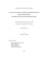
■ FIGURE 1.3

Summation of all the vectors of the magnetic
moments that make up the and spin state cones yields the
net magnetization vector M.

0.0000820 (only the first two terms of the Maclaurin power series
expansion are significant). Because 1/0.0000820 ϭ 12,200, we can
see that only one more spin out of every 24,400 spins will be in the
lower energy ( ) spin state.
The simple result is this: Cancellation of the nuclear magnetic
moments has the unfortunate result of causing approximately all but
2 of every (roughly) 50,000 spins to cancel each other (24,999 spins
in one spin state will cancel out the net effect of 24,999 spins in the
other spin state), leaving only 2 spins out of our ensemble of 50,000
spins to contribute the z-axis components to the net magnetization
vector M (see Figure 1.3).
Thus, for our ensemble of 4.2 quintillion spins, the number of
nuclear magnetic moments that we can imagine being lined up end
to end is reduced by a factor of 50,000 (25,000 for the excess number in the lower energy or spin state, and 2 for the fact that only
part of each nuclear magnetic moment is along the z-axis) to give
a final number of 1.7 ϫ 1014 spins or 170 trillion (in the UK, a 170
billion) spins. Even though 170 trillion is still a big number, nonetheless it is more than four orders of magnitude less than what we
might have first expected on the basis of looking at one spin.
Performing vector addition of the 170 trillion excess spins gives
us the net magnetization vector for our 5 mm sample containing
0.70 mL of 10 mM chloroform solution at 20°C in a 500 MHz NMR.

Ensemble. A large number of NMRactive spins.
Net magnetization vector, M. Syn.
magnetization. The vector sum of the
magnetic moments of an ensemble
of spins.

10

CHAPTER 1 Introduction

It is common to refer to this and comparable numbers of spins as an
ensemble.
Polarization. The unequal population of two or more spin states.

The net magnetization vector M is the entity we detect, but only M’s
component in the xy plane is detectable. Sometimes we refer to a
component of M simply as magnetization or polarization.

Signal-to-noise ratio, S/N. The
height of a real peak (measure from
the top of the peak to the middle of
the range of baseline noise) divided
by the amplitude of the baseline
noise over a statistically reasonable
range.

The gyromagnetic ratio affects the strength of the signal we observe
with an NMR spectrometer in three ways. One, the larger the , the
more spins will reside in the lower energy spin state (a Boltzmann
effect). Two, for each additional spin we get to drop into the lower
energy state, we add the magnitude of that spin’s nuclear magnetic
moment (which depends on ) to our net magnetization vector M
(a length-of- effect). Three, the precession frequency of M depends
on , so our detector will have less noise interfering with it. This last
point is the most difficult to understand, but it basically works as
follows: The higher the frequency of a signal, the easier it is to detect.

DC (direct current) signals are notoriously hard to make stable in
electronic circuitry, but AC (alternating current) signals are much
easier to generate stably. These three factors mean that the signal-tonoise ratio we obtain depends on the gyromagnetic ratio raised to
a power greater than two!

Radio frequency, RF. Electromagnetic radiation with a frequency range
from 3 kHz to 300 GHz.

Lattice. The rest of the world. The
environment outside the immediate
vicinity of a spin.

Once we have summed the behavior of individual spins into the net
magnetization vector M, we no longer have to worry about some of
the restrictions discussed earlier. In particular, the length of the vector or whether it is allowed to point in a particular direction is no
longer restricted. M can be manipulated with electromagnetic radiation in the radio-frequency range, often simply referred to as RF.
M can be tilted away from its equilibrium position along the z-axis
to point in any direction. The ability to visualize M’s movement
will become important later when we discuss RF pulses and pulse
sequences. For now, though, just try to accept that M can be tilted
from equilibrium and can grow or shrink depending on its interactions with other things, be they other spins, RF, or the lattice (the
rest of the world).
In other ways, however, the net magnetization vector M behaves
in a manner similar to the individual spins that it comprises. One
very important similarity has to do with how M will behave once it
is perturbed from its equilibrium position along the z-axis. M will
itself precess at the Larmor frequency if it has a component in the xy
plane (i.e., if it is no longer pointing in its equilibrium direction).
Detection of signal requires magnetization in the xy plane, because