Ebook Introduction to computational chemistry (2nd edition) Part 2
Bạn đang xem bản rút gọn của tài liệu. Xem và tải ngay bản đầy đủ của tài liệu tại đây (7.21 MB, 332 trang )
7
Valence Bond Methods
Essentially all practical calculations for generating solutions to the electronic
Schrödinger equation have been performed with molecular orbital methods. The
zeroth-order wave function is constructed as a single Slater determinant and the MOs
are expanded in a set of atomic orbitals, the basis set. In a subsequent step the wave
function may be improved by adding electron correlation with either CI, MP or CC
methods. There are two characteristics of such approaches: (1) the one-electron functions, the MOs, are delocalized over the whole molecule, and (2) an accurate treatment
of the electron correlation requires many (millions or billions) “excited” Slater determinants. The delocalized nature of the MOs is partly a consequence of choosing the
Lagrange multiplier matrix to be diagonal (canonical orbitals, eq. (3.42)), they may in
a subsequent step be mixed to form localized orbitals (see Section 9.4) without affecting the total wave function. Such a localization, however, is not unique. Furthermore,
delocalized MOs are at variance with the basic concept in chemistry that molecules
are composed of structural units (functional groups) which to a very good approximation are constant from molecule to molecule. The MOs for propane and butane, for
example, are quite different, although “common” knowledge is that they contain CH3
and CH2 units that in terms of structure and reactivity are very similar for the two molecules. A description of the electronic wave function as having electrons in orbitals
formed as linear combinations of all (in principle) atomic orbitals is also at variance
with the chemical language of molecules being composed of atoms held together by
bonds, where the bonds are formed by pairing unpaired electrons contained in atomic
orbitals. Finally, when electron correlation is important (as is usually the case), the need
to include many Slater determinants obscures the picture of electrons residing in
orbitals.
There is an equivalent way of generating solutions to the electronic Schrödinger
equation that conceptually is much closer to the experimentalist’s language, known as
Valence Bond (VB) theory.1 We will start by illustrating the concepts for the H2 molecule, and note how it differs from MO methods.
Introduction to Computational Chemistry, Second Edition. Frank Jensen.
© 2007 John Wiley & Sons, Ltd
7.1 CLASSICAL VALENCE BOND THEORY
269
7.1 Classical Valence Bond Theory
A single-determinant MO wave function for the H2 molecule within a minimum basis
consisting of a single s-function on each nucleus is given in eq. (7.1) (see also Section
4.3).
Φ0 =
f1(1) f1(1)
f1( 2) f1( 2)
f1 = ( c A + c B )a
(7.1)
f1 = ( c A + c B )b
We have here ignored the normalization constants. The Slater determinant may be
expanded in AOs, as shown in eq. (7.2).
Φ 0 = f1f1 − f1f1 = (f1f1 )[ab − ba ]
Φ 0 = ( c A + c B )( c A + c B )[ab − ba ]
(7.2)
Φ 0 = ( c A c A + c B c B + c A c B + c B c A )[ab − ba ]
This shows that the HF wave function consists of equal amounts of ionic (cAcA and
cBcB) and covalent (cAcB and cBcA) terms. In the dissociation limit only the covalent
terms are correct, but the single-determinant description does not allow the ratio of
covalent to ionic terms to vary. In order to provide a correct description, a second
determinant is necessary.
Φ1 =
f 2(1) f 2(1)
f 2( 2) f 2( 2)
f 2 = ( c A − c B )a
(7.3)
f 2 = ( c A − c B )b
Φ1 = ( c A c A + c B c B − c A c B − c B c A )[ab − ba ]
By including the doubly excited determinant Φ1, built from the antibonding MO, the
amounts of the covalent and ionic terms may be varied, and this is determined completely by the variational principle (eq. (4.20)).
ΨCI = a0 Φ 0 + a1Φ1
ΨCI = {(a0 − a1 )( c A c B + c B c A ) + (a0 + a1 )( c A c A + c B c B )}[ab − ba ]
(7.4)
This two-configurational CI wave function allows a qualitatively correct description of
the H2 molecule at all distances and in the dissociation limit, where the weights of the
two configurations become equal.
The classical VB wave function, on the other hand, is build from the atomic fragments by coupling the unpaired electrons to form a bond. In the H2 case, the two electrons are coupled into a singlet pair, properly antisymmetrized. The simplest VB
description, known as a Heitler–London (HL) function, includes only the two covalent
terms in the HF wave function.
Φ cov
HL = ( c A c B + c B c A )[ab − ba ]
(7.5)
Just as the single-determinant MO wave function may be improved by including
excited determinants, the simple VB-HL function may also be improved by adding
270
VALENCE BOND METHODS
terms that correspond to higher energy configurations for the fragments, in this case
ionic structures.
Φ ion
HL = ( c A c A + c B c B )[ab − ba ]
(7.6)
ion
ΨHL = a0 Φ cov
HL + a1 Φ HL
(7.7)
The final description, either in terms of a CI wave function written as a linear combination of two determinants build from delocalized MOs (eq. (7.4)), or as a VB wave function written in terms of two VB-HL structures composed of AOs (eq. (7.7)), is identical.
For the H2 system, the amount of ionic HL structures determined by the variational
principle is 44%, close to the MO-HF value of 50%. The need for including large
amounts of ionic structures in the VB formalism is due to the fact that pure atomic
orbitals are used.
Consider now a covalent VB function built from “atomic” orbitals that are allowed
to distort from the pure atomic shape.
Φ CF = (f Af B + f Bf A )[ab − ba ]
f A = c A + cc B
(7.8)
f B = c B + cc A
Such a VB function is known as a Coulson–Fischer (CF) type. The c constant is fairly
small (for H2, c is ~0.04), but by allowing the VB orbitals to adopt the optimum shape,
the need for ionic VB structures is strongly reduced. Note that the two VB orbitals in
eq. (7.8) are not orthogonal – the overlap is given by eq. (7.9).
f A f B = (1 + c 2 ) c A c B + 2c( c A c A + c B c B )
f A f B = (1 + c 2 )SAB + 4c
(7.9)
Compared with the overlap of the undistorted atomic orbitals used in the HL wave
function, which is just SAB, it is seen that the overlap is increased (c is positive), i.e. the
orbitals distort such that they overlap better in order to make a bond. Although the
distortion is fairly small (a few percent), this effectively eliminates the need for including ionic VB terms. When c is variationally optimized, the MO-CI, VB-HL and VB-CF
wave functions (eqs (7.4), (7.7) and (7.8)) are all completely equivalent. The MO
approach incorporates the flexibility in terms of an “excited” determinant, the VB-HL
in terms of “ionic” structures, and the VB-CF in terms of “distorted” atomic orbitals.
In the MO-CI language, the correct dissociation of a single bond requires the addition of a second doubly excited determinant to the wave function. The VB-CF wave
function, on the other hand, dissociates smoothly to the correct limit, the VB-orbitals
simply reverting to their pure atomic shapes, with the overlap disappearing.
7.2 Spin-Coupled Valence Bond Theory
The generalization of a Coulson–Fischer type wave function to the molecular case with
an arbitrary-size basis set is known as Spin-Coupled Valence Bond (SCVB) theory.2
It is again instructive to compare with the traditional MO approach, taking the CH4
molecule as an example. The MO single-determinant description (RHF, which is identical to UHF near the equilibrium geometry) of the valence orbitals is in terms of four
delocalized orbitals, each occupied by two electrons with opposite spin. The C—H
7.2 SPIN-COUPLED VALENCE BOND THEORY
271
bonding is described by four different, orthogonal molecular orbitals, each expanded
in a set of AOs.
4
Φ CH
valence-MO = A[f1f1f 2f 2f 3f 3f 4f 4 ]
fi =
M basis
∑c
ai
(7.10)
ca
a =1
Here A is the usual antisymmetrizer (eq. (3.21)) and a bar above a MO indicates that
the electron has a b spin function, no bar indicates an a spin function.
The SCVB description, on the other hand, considers the four bonds in CH4 as arising
from coupling of a single electron at each of the four hydrogen atoms with a single
unpaired electron at the carbon atom. Since the ground state of the carbon atom is a
triplet, corresponding to the electron configuration 1s22s22p2, the first step is formation
of four equivalent “hybrid” orbitals by mixing three parts p-function with one part sfunction, generating four equivalent “sp3-hybrid” orbitals. Each of these singly occupied hybrid orbitals can then couple with a hydrogen atom to form four equivalent
C—H bonds. The electron spins are coupled such that the total spin is a singlet, which
can be done in several different ways. The coupling of four electrons to a total singlet
state, for example, can be done either by coupling two electrons in a pair to a singlet,
and then coupling two singlet pairs, or by first coupling two electrons in a pair to a
triplet, and subsequently coupling two triplet pairs to an overall singlet.
+
4
+
Figure 7.1 Two possible schemes for coupling four electrons to an overall singlet
The Θ NS,i symbol is used to designate the ith combination of spin functions coupling
N electrons to give an overall spin of S, and there are f NS number of ways of doing this.
The value of f NS is given by eq. (7.11).
fSN =
( 2S + 1)N!
( N + S + 1)!( 12 N − S )!
(7.11)
1
2
For a singlet wave function (S = 0), the number of coupling schemes for N electrons
is given in Table 7.1.
Table 7.1 Number of possible spin coupling
schemes for achieving an overall singlet state
N
f N0
2
4
6
8
10
12
14
1
2
5
14
42
132
429
272
VALENCE BOND METHODS
For the eight valence electrons in CH4 there are 14 possible spin couplings resulting in an overall singlet state. The full SCVB function may be written (again neglecting normalization) as in eq. (7.12).
14
N
4
Φ CH
valence-SCVB = ∑ a i A{[f1f 2f 3f 4f 5f 6f 7f 8 ]Θ 0 ,i }
i =1
fi =
(7.12)
M basis
∑
cai c a
a =1
There are now eight different spatial orbitals, fi, four of which are essentially carbon
sp3-hybrid orbitals, with the other four being close to atomic hydrogen s-orbitals. The
expansion of each of the VB-orbitals in terms of all the basis functions located on all
the nuclei allows the orbitals to distort from the pure atomic shape. The SCVB wave
function is variationally optimized, both with respect to the VB-orbital coefficients cai
and the spin coupling coefficients ai. The result is that a complete set of optimum “distorted” atomic orbitals is determined together with the weight of the different spin
couplings. Each spin coupling term (in the so-called Rumer basis) is closely related to
the concept of a resonance structure used in organic chemistry textbooks. An SCVB
calculation of CH4 gives as a result that one of the spin coupling schemes completely
dominates the wave function, namely that corresponding to the electron pair in each
of the C—H bonds being singlet coupled. This is the quantum mechanical analogue of
the graphical representation of CH4 shown in Figure 7.2.
Each of the lines represents a singlet-coupled electron pair between two orbitals
that strongly overlap to form a bond, and the drawing in Figure 7.2 is the only important “resonance” form.
Figure 7.2 A representation of the dominating spin coupling in CH4
Consider now the π-system in benzene. The MO approach will generate linear combinations of the atomic p-orbitals, producing six π-orbitals delocalized over the whole
molecule with four different orbital energies (two sets of degenerate orbitals).
The stability of benzene can be attributed to the large gap between the HOMO and
LUMO orbitals.
A SCVB calculation considering only the coupling of the six π-electrons, gives a
somewhat different picture. The VB π-orbitals are strongly localized on each carbon,
resembling p-orbitals that are slightly distorted in the direction of the nearest neighbour atoms. It is now found that five spin coupling combinations are important, these
7.2 SPIN-COUPLED VALENCE BOND THEORY
273
Figure 7.3 Molecular orbital energies in benzene
Figure 7.4 Representations of important spin coupling schemes in benzene
are shown in Figure 7.4, where a bold line indicates two electrons coupled into a singlet
pair.
Each of the two first VB structures contributes ~40% to the wave function, and each
of the remaining three contributes ~6%.3 The stability of benzene in the SCVB picture
is due to resonance between these VB structures. It is furthermore straightforward to
calculate the resonance energy by comparing the full SCVB energy with that calculated from a VB wave function omitting certain spin coupling functions.
The MO wave function for CH4 may be improved by adding configurations corresponding to excited determinants, i.e. replacing occupied MOs with virtual MOs.
Allowing all excitations in the minimal basis valence space and performing the full
optimization corresponds to an [8,8]-CASSCF wave function (Section 4.6). Similarly,
the SCVB wave function in eq. (7.12) may be improved by adding ionic VB structures
such as CH3−/H+ and CH3+/H−, and this corresponds to exciting an electron from one
of the singly occupied VB orbitals into another VB orbital, thereby making it doubly
occupied. The importance of these excited/ionic terms can again be determined by the
variational principle. If all such ionic terms are included, the fully optimized SCVB+CI
wave function is for all practical purposes identical to that obtained by the MOCASSCF approach (the only difference is a possible slight difference in the description of the carbon 1s-core orbital).
Both types of wave function provide essentially the same total energy, and thus
include the same amount of electron correlation. The MO-CASSCF wave function
attributes the electron correlation to interaction of 1764 configurations, the
Hartree–Fock reference and 1763 excited configurations, with each of the 1763 configurations providing only a small amount of the correlation energy. The SCVB wave
function (which includes only one resonance structure), however, contains 90+% of
the correlation energy, and only a few percent is attributed to “excited” structures. The
ability of SCVB wave functions to include electron correlation is due to the fact that
the VB orbitals are strongly localized and, since they are occupied by only one electron, they have the built-in feature of electrons avoiding each other. In a sense, an
SCVB wave function is the best wave function that can be constructed in terms of prod-
274
VALENCE BOND METHODS
ucts of spatial orbitals. By allowing the orbitals to become non-orthogonal, the large
majority (80–90%) of what is called electron correlation in an MO approach can be
included in a single-determinant wave function composed of spatial orbitals, multiplied
by proper spin coupling functions.
There are a number of technical complications associated with optimizing the SCVB
wave function due to the non-orthogonal orbitals. The MO-CI or MO-CASSCF
approaches simplify considerably owing to the orthogonality of the MOs, and thereby
also of the Slater determinants. Computationally, the optimization of an SCVB wave
function, where N electrons are coupled in all possible ways, is similar to that required
for constructing an [N,N]-CASSCF wave function. This effectively limits the size of
SCVB wave functions to coupling of 12–16 electrons. The actual optimization of the
wave function is usually done by a second-order expansion of the energy in terms of
orbital and spin coupling coefficients, and employing a Newton–Raphson type scheme,
analogously to MCSCF methods (Section 4.6). The non-orthogonal orbitals have the
disadvantage that it is difficult to add dynamical correlation on top of an SCVB wave
function by perturbation or coupled cluster theory, although (non-orthogonal) CI
methods are straightforward. SCVB+CI approaches may also be used to describe
excited states, analogously to MO-CI methods.
It should be emphasized again that the results obtained from an [N,N]-CASSCF and
a corresponding N-electron SCVB wave function (or SCVB+CI and MRCI) are virtually identical. The difference is in the way the results can be analyzed. Molecules in
the SCVB picture are composed of atoms held together by bonds, where bonds are
formed by (singlet) coupling of the electron spins between (two) overlapping orbitals.
These orbitals are strongly localized, usually on a single atom, and are basically atomic
orbitals slightly distorted by the presence of the other atoms in the molecule. The VB
description of a bond as the result of two overlapping orbitals is in contrast to the MO
approach where a bond between two atoms arises as a sum over (small) contributions
from many delocalized molecular orbitals. Furthermore, the weight of the different
ways spin couplings in an SCVB wave function carries a direct analogy with chemical
concepts such as “resonance” structures.
The SCVB method is a valuable tool for providing insight into the problem. This is
to a certain extent also possible from an MO type wave function by localizing the
orbitals or by analyzing the natural orbitals (see Sections 9.4 and 9.5 for details).
However, there is no unique method for producing localized orbitals, and different
methods may give different orbitals. Natural orbitals are analogous to canonical
orbitals delocalized over the whole molecule. The SCVB orbitals, in contrast, are
uniquely determined by the variational procedure, and there is no freedom to further
transforming them by making linear combinations without destroying the variational
property.
The primary feature of SCVB is the use of non-orthogonal orbitals, which allows a
much more compact representation of the wave function. An MO-CI wave function
of a certain quality may involve many thousands of Slater determinants, while a similarquality VB wave function may be written as only a handful of “resonating” VB structures. Furthermore, the VB orbitals, and spin couplings, of a C—H bond in say propane
and butane are very similar, in contrast to the vastly different MO descriptions of the
two systems. The VB picture is thus much closer to the traditional descriptive language
used with molecules composed of functional groups. The widespread availability of
7.3 GENERALIZED VALENCE BOND THEORY
275
programs for performing CASSCF calculations, and the fact that CASSCF calculations
are computationally more efficient owing to the orthogonality of the MOs, have
prompted developments of schemes for transforming CASSCF wave functions to VB
structures, denoted CASVB.3 A corresponding procedure using orthogonal orbitals
(which introduce large weights of ionic structures) has also been reported.4
7.3 Generalized Valence Bond Theory
The SCVB wave function allows all possible spin couplings to take place and has no
restrictions on the form of the orbitals. The Generalized Valence Bond (GVB) method
can be considered as a reduced version of the full problem where only certain subsets
of spin couplings are allowed.5 For a typical case of a singlet system, the GVB method
has two (non-orthogonal) orbitals assigned to each bond, and each pair of electrons in
a bond are required to couple to a singlet pair. The coupling of such singlet pairs will
then give the overall singlet spin state. This is known as Perfect Pairing (PP), and is one
of the many possible spin coupling schemes, and such two-electron two-orbital pairs
are called geminal pairs. Just as an orbital is a wave function for one electron, a geminal
is a wave function for two electrons. In order to reduce the computational problem,
the Strong Orthogonality (SO) condition is normally imposed on the GVB wave function. This means that orbitals belonging to different pairs are required to be orthogonal. While the perfect pairing coupling typically is the largest contribution to the full
SCVB wave function, the strong orthogonality constraint is often a quite poor approximation, and may lead to artefacts. For diazomethane, for example, the SCVB wave
function is dominated (91%) by the PP coupling, leading to the conclusion that the
molecule has essentially normal C=N and N=N π-bonds, perpendicular to the plane
defined by the CH2 moiety.6 Taking into account also the in-plane bonding, this suggest
that diazomethane is best described with a triple bond between the two nitrogens,
thereby making the central nitrogen “hypervalent”, as illustrated in Figure 7.5.
Figure 7.5 A representation of the SCVB wave function for diazomethane
There are strong overlaps between the VB orbitals, the smallest overlap (between
the carbon and terminal nitrogen) is ~0.4, and that between the two orbitals on the
central nitrogen is ~0.9. The GVB-SOPP approach, however, forces these geminal
pairs to be orthogonal, leading to the conclusion that the electronic structure of
diazomethane has a very strong diradical nature, as illustrated in Figure 7.6.
Figure 7.6 A representation of the GVB wave function for diazomethane
276
VALENCE BOND METHODS
References
1. S. Shaik, P. C. Hiberty, Rev. Comp. Chem., 20 (2004), 1.
2. D. L. Cooper, J. Gerratt, M. Raimondi, Chem. Rev., 91 (1991), 929; J. Gerratt, D. L. Cooper,
P. B. Karadakov, M. Raimondi, Chem. Soc. Rev., 26 (1997), 87.
3. D. L. Cooper, T. Thorsteinsson, J. Gerratt, Int. J. Quant. Chem., 65 (1997), 439.
4. K. Hirao, H. Nakano, K. Nakayama, M. Dupuis, J. Chem. Phys., 105 (1996), 9227.
5. W. A. Goddard III, L. B. Harding, Ann. Rev. Phys. Chem., 29 (1978), 363.
6. D. L. Cooper, J. Gerratt, M. Raimondi, S. C. Wright, Chem. Phys. Lett., 138 (1987), 296.
8
Relativistic Methods
The central theme in relativity is that the speed of light, c, is constant in all inertia
frames (coordinate systems that move with respect to each other). Augmented with
the requirement that physical laws should be identical in such frames, this has as a consequence that time and space coordinates become “equivalent”. A relativistic description of a particle thus requires four coordinates, three space and one time coordinate.1
The latter is usually multiplied by c to have units identical to the space variables.
A change between different coordinate systems can be described by a Lorentz transformation, which may mix space and time coordinates. The postulate that physical laws
should be identical in all coordinate systems is equivalent to the requirement that
equations describing the physics must be invariant (unchanged) to a Lorentz transformation. Considering the time-dependent Schrödinger equation (8.1), it is clear that
it is not Lorentz invariant since the derivative with respect to space coordinates is of
second order, but the time derivative is only first order. The fundamental structure of
the Schrödinger equation is therefore not relativistically correct.
2
2
2
− 1 ∂ + ∂ + ∂ + V Ψ = i ∂Ψ
2 m ∂x 2 ∂y 2 ∂z2
∂t
(8.1)
For use below, we have elected here to explicitly write the electron mass as m, although
it is equal to one in atomic units.
One of the consequences of the constant speed of light is that the mass of a particle,
which moves at a substantial fraction of c, increases over the rest mass m0.
v2
m = m0 1 − 2
c
−1
(8.2)
The energy of a 1s-electron in a hydrogen-like system (one nucleus and one electron)
is −Z2/2, and classically this is equal to minus the kinetic energy, 1/2mv2, owing to the
virial theorem (E = −T = 1/2V). In atomic units (m = 1) the classical velocity of a 1selectron is thus Z. The speed of light in atomic units is 137.036, and it is clear that
relativistic effects cannot be neglected for the core electrons in heavy nuclei. For atoms
with large Z, the 1s-electrons are relativistic and thus heavier, which has the effect that
Introduction to Computational Chemistry, Second Edition. Frank Jensen.
© 2007 John Wiley & Sons, Ltd
278
RELATIVISTIC METHODS
the 1s-orbital shrinks in size, by the same factor as the mass increases (eq. (8.2)). In
order to maintain orthogonality, the higher s-orbitals also contract. This provides a
more effective screening of the nuclear charge for the higher angular momentum
orbitals, which consequently increase in size. For p-orbitals the spin–orbit interaction,
which mixes s- and p-orbitals, counteracts the inflation. The net effect is that p-orbitals
are relatively unaffected in size, while d- and f-orbitals become larger and more diffuse.
In terms of total energy, the relativistic correction becomes comparable to the correlation energy already for Z~10, while it becomes comparable to the exchange energy
for Z~50. Since the majority of the relativistic effects are concentrated in the core
orbitals, there is a large error cancellation for molecular properties. Relativistic effects
for geometries and energetics are normally negligible for the first three rows in the
periodic table (up to Kr, Z = 36, corresponding to a “mass correction” of 1.04), the
fourth row represents an intermediate case, while relativistic corrections are necessary
for the fifth and sixth rows, and for lanthanide/actinide metals. For effects involving
electron spin (e.g. spin–orbit coupling), which are purely relativistic in origin, there is
no non-relativistic counterpart, and the “relativistic correction” is of course everything.
Although an in-depth treatment of relativistic effects is outside the scope of this
book, it may be instructive to point out some of the features and problems in a relativistic quantum description of atoms and molecules. Furthermore, we will require
some operators derived from a relativistic treatment for calculating molecular properties in Chapter 10.
8.1 The Dirac Equation
For a free electron, Dirac proposed that the (time-dependent) Schrödinger equation
should be replaced by eq. (8.3).
[ca ⋅ p + bmc 2 ]Ψ = i
∂Ψ
∂t
(8.3)
Here a and b are 4 × 4 matrices, a is written in terms of the three Pauli 2 × 2 spin
matrices s, and b in term of a 2 × 2 unit matrix I.
a x , y, z =
0
s x , y, z
0 1
sx =
1 0
s x , y, z
0
I 0
b=
0 I
0 −i
sy =
i 0
1 0
sz =
0 −1
(8.4)
1 0
I=
0 1
Except for a factor of 1/2, the sx,y,z matrices can be viewed as representations of the sx,
sy and sz spin operators, respectively, when the a and b spin functions are taken as (1,0)
and (0,1) vectors.
s z = 12 s z
1
1
s z = 12
0
0
0
0
s z = − 12
1
1
(8.5)
8.1 THE DIRAC EQUATION
279
The a function is an eigenfunction of the sz operator with an eigenvalue of 1/2, and the
b function similarly has an eigenvalue of −1/2.
The Dirac equation is of same order in all variables (space and time), since the
momentum operator p (= −i∇) involves a first-order differentiation with respect to the
space variables. It should be noted that the free electron rest energy in eq. (8.3) is mc2,
equal to 0.511 MeV, while this situation is defined as zero in the non-relativistic case.
The zero point of the energy scale is therefore shifted by 5.11 × 10⁵ eV, a large amount
compared with the binding energy of 13.6 eV for a hydrogen atom. The two (relativistic and non-relativistic) energy scales may be aligned by subtracting the electron rest
energy, which corresponds to replacing the b matrix in eq. (8.3) by b¢.
0 0
b′ =
0 2I
(8.6)
The Dirac equation corresponds to satisfying the requirements of special relativity in
connection with the quantum behaviour of the electron. Special relativity considers
only systems that move with a constant velocity with respect to each other, which can
hardly be considered a good approximation for the movement of an electron around
a nucleus. A relativistic treatment of accelerated systems is described by general relativity, which is a gravitational theory. For atomic systems, however, the gravitational
interaction between electrons and nuclei (or between electrons) is insignificant compared with the electrostatic interaction. Furthermore, a consistent theory describing
the quantum aspects of gravitation has not yet been developed.
The Dirac equation is four-dimensional, and the relativistic wave function consequently contains four components. Two of the degrees of freedom are accounted for
by assigning an intrinsic magnetic moment (spin), while the other two are interpreted as two different particles, electron and positron. The positronic solutions show
up as a continuum of “negative” energy states, having energies below −2mc2,
as illustrated in Figure 8.1. Note that the spacing between bound states has been
exaggerated, as the binding energy is of the order of eV while 2mc2 is of the order of
MeV.
Non-relativistic
Relativistic
Continuum
Discrete
states
Electronic
states
Energy
0
–2mc2
Continuum
Figure 8.1 Non-relativistic and relativistic solutions
Positronic
states
280
RELATIVISTIC METHODS
It is conventional to write the relativistic wave function as in eq. (8.7).
ΨLa
ΨLb
Ψ=
ΨSa
ΨSb
(8.7)
Here ΨL and ΨS are the large and small components of the wave function, and a and
b indicate the usual spin functions. Note that the spatial parts of ΨLa/ΨLb, and ΨSa/ΨSb,
are not necessarily identical. For electrons, the large component reduces to the solutions of the Schrödinger equation when c → ∞ (the non-relativistic limit), and the small
component disappears. The small component of the electronic wave function corresponds to a coupling with the positronic states.
8.2 Connections Between the Dirac and Schrödinger Equations
8.2.1 Including electric potentials
In the presence of an electric potential V (e.g. from nuclei), the time-independent Dirac
equation may be written as in eq. (8.8), where we have again explicitly indicated the
electron mass.
[ca ⋅ p + b ′mc 2 + V]Ψ = EΨ
(8.8)
Since a and b¢ are block matrices in terms of s and I, eq. (8.8) can be factored out in
two equations.
c(s ⋅ p)ΨS + VΨL = EΨL
c(s ⋅ p)ΨL + ( −2 mc 2 + V)ΨS = EΨS
(8.9)
Here ΨL and ΨS are (large and small) two-component wave functions that include the
a and b spin functions. The latter equation can be solved for ΨS.
−1
ΨS = (E + 2 mc 2 − V) c(s ⋅ p)ΨL
(8.10)
The inverse quantity can be factorized as in eq. (8.11).
−1
−1
−1
−1
E − V
= ( 2 mc 2 ) K
(E + 2 mc 2 − V) = ( 2 mc 2 ) 1 +
2
2 mc
E − V
K = 1 +
2 mc 2
−1
(8.11)
Eq. (8.10) may then be written as in eq. (8.12).
ΨS = K
s ⋅p
ΨL
2mc
(8.12)
The top equation in (8.9) then becomes eq. (8.13).
1 (s ⋅ p)K(s ⋅ p) + ( V − E ) Ψ = 0
2 m
L
(8.13)
8.2 CONNECTIONS BETWEEN THE DIRAC AND SCHRÖDINGER EQUATIONS
281
In the non-relativistic limit (c → ∞) the K factor is 1, and the first term becomes
(s ⋅ p)(s ⋅ p). Using the vector identity (s ⋅ p)(s ⋅ p) = p ⋅ p + is(p × p), this gives the nonrelativistic kinetic energy p2/2m, since the vector product of any vector with itself is
zero (p × p = 0). The equation for the large component therefore reduces to the
Schrödinger equation.
2
p + V Ψ = EΨ
L
2m
L
(8.14)
The electron spin is still present in eq. (8.14), since ΨL is a two-component wave function, but this can trivially be separated out since the operators do not contain any spin
dependence.
In the non-relativistic limit the small component of the wave function is given by
eq. (8.15).
ΨS =
s ⋅p
ΨL
2mc
(8.15)
For a hydrogenic wave function (ΨL ≈ e−Zr), this gives eq. (8.16) in atomic units (setting
m = 1).
ΨS ≈
Z
ΨL
2c
(8.16)
For a hydrogen atom the small component accounts for only ~0.4% of the total wave
function and 10−3% of the electron density, but for a uranium 1s-electron it is a third
of the wave function and ~10% of the density.
We may obtain relativistic corrections by expanding the K factor in eq. (8.11).
E − V
K = 1 +
2 mc 2
−1
≈ 1−
E−V
+...
2 mc 2
(8.17)
This is only valid when E − V << 2mc2, however all atoms have a region close to the
nucleus where this is not fulfilled (since V → −∞ for r → 0). Inserting (8.17) in (8.13),
assuming a Coulomb potential −Z/r (i.e. V is the attraction to a nucleus), gives after
renormalization of the (large component) wave function and some rearrangement the
terms shown in eq. (8.18).
2
4
Zs ⋅ I
Zpd (r )
p +V− p
ΨL = EΨL
+
+
3 2
2 m
8m c
2 m 2 c 2 r 3 2 m 2 c 2
(8.18)
Eq. (8.18) is called the Pauli equation. The first two terms are the usual nonrelativistic kinetic and potential energy operators, the p4 term is called the mass–
velocity correction, and is due to the dependence of the electron mass on the
velocity. The next is the spin–orbit term (s is the electron spin and l is the angular
momentum operator r × p), which corresponds to an interaction of the electron
spin with the magnetic field generated by the movement of the electron. The
last term involving the δ function is the Darwin correction, which corresponds to a
correction that can be interpreted as the electron making a high-frequency oscillation
around its mean position, sometimes referred to as Zwitterbewegung. The mass–
velocity and Darwin corrections are often collectively called the scalar relativistic
282
RELATIVISTIC METHODS
corrections. Since they have opposite signs, they do to a certain extent cancel each
other.
Owing to the divergence of the K expansion near the nuclei, the mass–velocity and
Darwin corrections can only be used as first-order corrections. Inclusion of such operators in a variational sense will result in a collapse of the wave function. An alternative
method is to partition eq. (8.11) as in eq. (8.19), which avoids the divergence near the
nucleus.
−1
−1
(E + 2 mc 2 − V) = ( 2 mc 2 − V) 1 +
E
K′ = 1 +
2 mc 2 − V
E
2 mc 2 − V
−1
−1
= ( 2 mc 2 − V) K ′
−1
(8.19)
In contrast to eq. (8.17), the factor E/(2mc2 − V) is always much smaller than 1, and
K¢ may be expanded in powers of E/(2mc2 − V), analogously to eq. (8.17). Keeping
only the zeroth-order term (i.e. setting K¢ = 1) gives the Zeroth-Order Regular Approximation (ZORA) method, eq. (8.20).2
c 2p2
Zs ⋅ I
2c 2
+
− 3 + V ΨL = EΨL
2
2
r
2 mc − V ( 2 mc 2 − V)
(8.20)
Note that in this case the spin–orbit coupling is already included in zeroth order.
Including the first-order term from an expansion of K¢ defines the First-Order Regular
Approximation (FORA) method. A disadvantage of these methods is that they are not
gauge invariant.3
8.2.2 Including both electric and magnetic potentials
The presence of a magnetic field can be included in the so-called minimal coupling by
addition of a vector potential A to the momentum operator p, forming a generalized
momentum operator p, which for an electron (charge of −1) is given by eq. (8.21).
p = p+A
(8.21)
The magnetic field is defined as the curl of the vector potential.
B=∇×A
(8.22)
For an external magnetic field, it is conventional to write the vector potential as in eq.
(8.23).
A(r ) = 12 B × (r − R G )
(8.23)
Here RG is the gauge origin, i.e. the “zero” point for the vector potential. The
gauge origin is often taken as the centre of mass for the system, but this is by no
means unique. The results from an exact calculation will be independent of RG but, for
approximate calculations, this is not guaranteed, and the results may thus depend on
where the gauge origin is chosen. Such gauge-dependent properties are clearly undesirable, since different values can be generated by selecting different (arbitrary) gauge
origins.
8.2 CONNECTIONS BETWEEN THE DIRAC AND SCHRÖDINGER EQUATIONS
283
With the generalized momentum operator p replacing p, the time-independent Dirac
equation may be separated analogously to the procedure in Section 8.2.1 to give the
equivalent of eq. (8.13).
1 (s ⋅ p )K(s ⋅ p ) + ( V − E ) Ψ = 0
2 m
L
(8.24)
Taking the non-relativistic limit corresponding to K = 1 gives (s ⋅ p)(s ⋅ p) for the first
term. Using again the vector identity (s ⋅ p)(s ⋅ p) = p ⋅ p + is(p × p), this may be written
as in eq. (8.25).
1 ( p ⋅ p + is ⋅ ( p × p )) + V Ψ = EΨ
L
L
2m
(8.25)
In contrast to the situation without a magnetic field, the latter vector product no longer
disappears. The p × p term can be expanded by inserting the definition of p from eq.
(8.21).
p × p = (p + A ) × (p + A )
= p× p+p× A +A × p+A × A
(8.26)
The first and last terms are zero (since a × a = 0). With p = −i∇ the other two terms
yield eq. (8.27).
(p × A + A × p)Ψ = −i∇ × (AΨ) − iA × (∇Ψ)
= −i(∇ × A )Ψ − i(∇Ψ ) × A − iA × (∇Ψ )
(8.27)
The two last terms cancel (since a × b = −b × a), and the curl of the vector potential is
the magnetic field, eq. (8.22). The final result is given in eq. (8.28).
p + V + s ⋅ B Ψ = EΨ
L
L
2 m
2 m
2
(8.28)
The s ⋅ B term is called the (spin) Zeeman interaction, and represents the interaction
of an (external) magnetic field with the intrinsic magnetic moment associated with the
electron. As noted in eq. (8.5), s represents the spin operator (except for a factor of
1/ ), and the s ⋅ B/2m interaction can (in atomic units) also be written as s ⋅ B, with s
2
being the electron spin operator. In a more refined treatment, by including quantum
field corrections, it turns out that the electron magnetic moment is not exactly equal
to the spin. It is conventional to write the interaction as gemBs ⋅ B where the Bohr magneton mB (= eh-/2m) has a value of 1/2 in atomic units and the electronic g-factor ge is
approximately equal to 2.0023 (the deviation from the value of 2 (exactly) is due to
quantum field fluctuations).
Although electron spin is often said to arise from relativistic effects, the above shows
that spin naturally arises in the non-relativistic limit of the Dirac equation. It may also
be argued that electron spin is actually present in the non-relativistic case, as the kinetic
energy operator p2/2m is mathematically equivalent to (s ⋅ p)2/2m. If the kinetic energy
is written as (s ⋅ p)2/2m in the Schrödinger Hamiltonian, then electron spin is present
in the non-relativistic case, although it would only have consequences in the presence
of a magnetic field.
284
RELATIVISTIC METHODS
The Dirac equation automatically includes effects due to electron spin, while this
must be introduced in a more or less ad hoc fashion in the Schrödinger equation (the
Pauli principle). Furthermore, once the spin–orbit interaction is included, the total electron spin is no longer a “good” quantum number: an orbital no longer contains an
integer number of a and b spin functions. The proper quantum number in relativistic
theory is therefore the total angular momentum obtained by vector addition of the
orbital and spin moments.
Turning now to the p2 term in eq. (8.28), it can with the use of eq. (8.21) be expanded
into eq. (8.29).
2
p 2 = (p + A ) = p 2 + p ⋅ A + A ⋅ p + A 2
(8.29)
The p gives the usual (non-relativistic) kinetic energy operator. Since p = −i∇, the
p ⋅ A term gives eq. (8.30).
2
(p ⋅ A )Ψ = −i(∇⋅ A )Ψ = −iA ⋅ (∇Ψ) − iΨ(∇⋅ A )
(8.30)
The Coulomb gauge is defined by ∇ ⋅ A = 0, and in this gauge we have p ⋅ A = A ⋅ p. The
two terms involving A in eq. (8.29) can be evaluated by inserting the expression for
the vector potential (8.23).
A ⋅ p = ( 12 B × (r − R G )) ⋅ p
= 12 B ⋅ (r − R G ) × p
= 12 B ⋅ L G
(8.31)
A 2 = ( 12 B × (r − R G )) ⋅ ( 12 B × (r − R G ))
=
1
4
(B 2 ⋅ (r − R G )) − (B ⋅ (r − R G ))
2
2
Here the vector identities a × b⋅c = a⋅b × c and (a × b)⋅(c × d) = (a⋅c)(b⋅d) − (a⋅d)(c⋅b)
have been used. In addition to the Zeeman term for electron spin (eq. (8.28)), the presence of a magnetic field introduces two new terms, being linear and quadratic in the
field. The linear operator represents an (orbital) Zeeman type interaction of the magnetic field with the magnetic moment generated by the movement of the electron, as
described by the angular momentum operator LG, while the quadratic term gives rise
to a component of the magnetizability in a perturbation treatment, as discussed in
Section 10.7.6.
8.3 Many-Particle Systems
A fully relativistic treatment of more than one particle would have to start from a full
QED treatment of the system (Chapter 1), and perform a perturbation expansion in
terms of the radiation frequency. There is no universally accepted way of doing
this, and a full relativistic many-body equation has not yet been developed. For manyparticle systems it is assumed that each electron can be described by a Dirac operator
(ca ⋅ p + b¢mc2) and the many-electron operator is a sum of such terms, in analogy with
the kinetic energy in non-relativistic theory. Furthermore, potential energy operators
are added to form a total operator equivalent to the Hamiltonian operator in nonrelativistic theory. Since this approach gives results that agree with experiments, the
assumptions appear justified.
8.3 MANY-PARTICLE SYSTEMS
285
The Dirac operator incorporates relativistic effects for the kinetic energy. In order
to describe atomic and molecular systems, the potential energy operator must also
be modified. In non-relativistic theory, the potential energy is given by the Coulomb
operator.
V(r12 ) =
q1q2
r12
(8.32)
According to this equation, the interaction between two charged particles depends
only on the distance between them, but not on time. This cannot be correct when relativity is considered, as it implies that the attraction/repulsion between two particles
occurs instantly over the distance r12, violating the fundamental relativistic principle
that nothing can move faster than the speed of light. The interaction between distant
particles must be “later” than between particles that are close, and the potential is consequently “retarded” (delayed). The relativistic interaction requires a description,
Quantum ElectroDynamics (QED), which involves exchange of photons between
charged particles. The photons travel at the speed of light and carry the information
equivalent to the classical Coulomb interaction. The relativistic potential energy
operator becomes complicated and cannot be written in closed form. For actual calculations, it may be expanded in a Taylor series in 1/c and, for chemical purposes, it is
normally only necessary to include terms up to 1/c2. In this approximation, the potential energy operator for the electron–electron repulsion is given by eq. (8.33).
Vee(r12 ) =
1
1
−
r12 r12
a ⋅ a + (a 1 × r12 )(a 2 × r12 )
1 2
r122
(8.33)
Note that the subscript on the a-matrices refers to the particle, and a here includes all
of the ax, ay and az components in eq. (8.4). The first correction term in the square
bracket is called the Gaunt interaction, and the whole term in the square bracket
is the Breit interaction. The Dirac matrices appear since they represent the velocity
operators in a relativistic description. The Gaunt term is a magnetic interaction (spin)
while the other term represents a retardation effect. Equation (8.33) is more often
written in the form shown in eq. (8.34).
VeeCoulomb− Breit(r12 ) =
1
1
−
r12 2r12
a ⋅ a + (a 1 ⋅ r12 )(a 2 ⋅ r12 )
1 2
r122
(8.34)
Relativistic corrections to the nuclear–electron attraction (Vne) are of order 1/c3 (owing
to the much smaller velocity of the nuclei) and are normally neglected.
An expansion in powers of 1/c (or, equivalently, in powers of the fine-structure
constant a = 1/c in atomic units) is a standard approach for deriving relativistic
correction terms. Taking into account electron (s) and nuclear spins (I), and
indicating explicitly an external electric potential by means of the field (F = −∇f, or
−∇f − ∂A/∂t if time dependent), an expansion up to order 1/c2 of the Dirac Hamiltonian including the Coulomb–Breit potential gives the following set of operators,4
where the QED correction to the electron spin has been introduced by means of the
gemB factor. Note that many of these operators arise from the minimal coupling of the
magnetic field via the generalized momentum operator, as discussed in more detail in
Section 10.10.7.
286
RELATIVISTIC METHODS
One electron operators:
N elec
∑ s ⋅B
H Zeeman
= ge m B
e
i
i
1
(s i ⋅ Bi )p i2
2 mc 2
−
i =1
1
H mv
e = −
8 m3 c 2
H SO
e = −
ge m B
4 mc 2
N elec
∑p
4
i
i =1
N elec
∑ [si ⋅ p i × Fi − si ⋅ Fi × p i ]
(8.35)
i =1
1
=−
H Darwin
e
8m2c 2
N elec
∑ ∇ ⋅F
i
i =1
Here Fi and Bi indicate the (electric and magnetic) fields at the position of particle i.
H Zeeman
has the s ⋅ B term from eq. (8.28) and a relativistic correction, and H mv
e
e is the
Darwin
mass–velocity correction, as is also present in eq. (8.18). H SO
are spin–orbit
e and H e
and Darwin type correction with respect to an external electric field. It should be noted
that the generalized momentum operator contains magnetic fields via the vector potential p = p + A, and eq. (8.35) therefore implicitly includes higher order effects.
Two electron operators:
H SO
ee = −
=−
H SOO
ee
ge m B
2 mc 2
ge m B
mc 2
ge2 m B2
H SS
ee =
2c 2
H OO
ee = −
=−
H Darwin
ee
s i ⋅ (rij × pi )
rij3
N elec N elec
∑∑
i =1
j ≠i
N elec N elec
∑∑
i =1
j ≠i
N elec N elec
∑ ∑
i =1
j ≠i
s i ⋅ (rij × p j )
rij3
si ⋅ s j
(s i ⋅ rij )(rij ⋅ s j ) 8p
−3
−
(s i ⋅ s j )d (rij )
3
3
rij
rij5
1
4m2c 2
N elec N elec
p
2m2c 2
N elec N elec
∑ ∑
i =1
j ≠i
(8.36)
p i ⋅ p j ( p i ⋅ rij )(rij ⋅ p j )
+
rij
rij3
∑ ∑ d (r )
ij
i =1
j ≠1
The sums run over all values of i and j, excluding the i = j term, and there is consequently a factor of 1/2 included to avoid overcounting. H SO
ee is a spin–orbit operator,
describing the interaction of the electron spin with the magnetic field generated by its
own movement, as given by the angular momentum operator rij × pi. H SOO
is a
ee
spin–other-orbit operator, describing the interaction of an electron spin with the magnetic field generated by the movement of the other electrons, as given by the angular
OO
momentum operator rij × pj. H SS
ee and H ee are spin–spin and orbit–orbit terms, accounting for additional magnetic interactions, where the orbit–orbit term comes from the
Breit correction to Vee (eq. (8.34)). The (two-electron) Darwin interaction H Darwin
conee
tains a δ function, which arise from the divergence of the field (∇ ⋅ F) from the
(electron–electron) potential energy operator, i.e. ∇ ⋅ (∇(1/r)) = −4πδ(r). The spin–spin
interaction H SS
ee also has a δ function, which comes from taking the curl of the vector
potential associated with the magnetic dipole corresponding to the electron spin. A
mathematical reformulation leads to a term involving the divergence of the r/r3
8.4 FOUR-COMPONENT CALCULATIONS
287
operator, giving ∇ ⋅ (r/r3) = (4π/3)δ(r). Such terms are often called contact interactions,
since they depend on the two particles being at the same position (r = 0). In the
spin–spin case, it is normally called the Fermi Contact (FC) term.
Operators involving one nucleus and one electron:
H SO
ne =
ge m B
2 mc 2
m
PSO
= N2
H ne
mc
N elec N nuclei
∑ ∑
i =1
ZA
A =1
N elec N nuclei
∑ ∑
i =1
A =1
ge m B m N
H SS
ne = −
c2
p
H Darwin
=
ne
2m2c 2
gA
∑ ∑
i =1
∑ ∑
i =1
I A ⋅ (riA × pi )
riA3
N elec N nuclei
A =1
N elec N nuclei
s i ⋅ (riA × p i )
riA3
s ⋅I
(s ⋅ r )(r ⋅ I ) 8p
g A i 3 A − 3 i iA 5 iA A −
(s i ⋅ I A )d (riA )
riA
3
riA
(8.37)
Z Ad (riA )
A =1
The H SO
ne operator is the one-electron part of the spin–orbit interaction, while the
H SO
and
H SOO
operators in eq. (8.36) define the two-electron part. The one-electron
ee
ee
term dominates and the two-electron contribution is often neglected or accounted
SO
for approximately by introducing an effective nuclear charge in H ne
(corresponding
to a screening of the nucleus by the electrons). The effect of the spin–orbit operators
is to mix states having different total spin, as for example singlet and triplet
states.
The equivalent of the spin–other-orbit operator in eq. (8.36) splits into two contributions, one involving the interaction of the electron spin with the magnetic field generated by the movement of the nuclei, and one describing the interaction of the nuclear
spin with the magnetic field generated by the movement of the electrons. Only the
latter survives within the Born–Oppenheimer approximation, and it is normally
denoted the Paramagnetic Spin–Orbit (PSO) operator. The spin–spin term is analogous
to that in eq. (8.36), while the term describing the orbit–orbit interaction disappears
owing to the Born–Oppenheimer approximation. The spin–orbit and (one-electron)
Darwin terms are the same as given in eq. (8.18), except for the quantum field
correction factor of gemB.
All of the terms in eqs (8.35)–(8.37) may be used as perturbation operators in connection with non-relativistic theory,5 as discussed in more detail in Chapter 10. It should
be noted, however, that some of the operators are inherently divergent and should not
be used beyond a first-order perturbation correction.
8.4 Four-Component Calculations
Although relativistic effects can be included by perturbative operators describing
corrections to the non-relativistic wave function, this rapidly becomes cumbersome
if higher order corrections are required, and it is then perhaps more satisfying to
include relativistic effects by solving the Dirac equation directly. The simplest approximative wave function is a single determinant constructed from four-component oneelectron functions, called spinors, having large and small components multiplied with
the two spin functions. The spinors are the relativistic equivalents of the spin-orbitals
in non-relativistic theory. With such a wave function, the relativistic equation
288
RELATIVISTIC METHODS
corresponding to the Hartree–Fock equation is the Dirac–Fock equation, which in its
time-independent form (setting p = p and m = 1 in eq. (8.8)) can be written as in
eq. (8.38).
[ca ⋅ p + b ′c 2 + V]Ψ = EΨ
(8.38)
The requirement that the wave function should be stationary with respect to a variation in the orbitals, results in an equation that is formally the same as in non-relativistic
theory, FC = SCe (eq. (3.51)). However, the presence of solutions for the positronic
states means that the desired solution is no longer the global minimum (Figure 8.1),
and care must be taken that the procedure does not lead to variational collapse. The
choice of basis set is an essential component in preventing this. Since practical calculations necessarily use basis sets that are far from complete, the large and small component basis sets must be properly balanced. The large component corresponds to the
normal non-relativistic wave function, and has similar basis set requirements. The small
component basis set is chosen to obey the kinetic balance condition, which follows from
(8.15).
c small =
s ⋅ p large
c
2c
(8.39)
The use of kinetic balance ensures that the relativistic solution smoothly reduces to
the non-relativistic wave function as c is increased. The presence of the momentum
operator in eq. (8.39) means that the small component basis set must contain functions
that are derivatives of the large component basis set, making the former roughly twice
the size of the latter. This means that there are ~8 times as many large–small twoelectron integrals and ~16 times as many small–small integrals, than there are
large–large type integrals. A relativistic calculation thus requires roughly 25 times as
many two-electron integrals compared with a non-relativistic calculation.
When the Dirac operator is invoked, the point charge model of the nucleus also
becomes problematic. For a non-relativistic hydrogen atom, the orbitals have a cusp
(discontinuous derivative) at the nucleus. However, the relativistic solutions have a singularity. A singularity is much harder to represent in an approximate treatment (such
as an expansion in a Gaussian basis) than a cusp. Consequently, a (more realistic) finitesize nucleus is often used in relativistic methods. A finite nucleus model removes the
singularity of the orbitals, which now assume a Gaussian type behaviour within the
nucleus. Neither experiments nor theory, however, provide a good model for how
the positive charge is distributed within the nucleus. The wave function and energy will
of course depend on the exact form used for describing the nuclear charge distribution. A popular choice is either a uniformly charged sphere, where the radius is proportional to the nuclear mass to the 1/3 power, or a Gaussian charge distribution (which
facilitates the calculation of the additional integrals) with the exponent depending on
the nuclear mass. Note that this implies that the energy (and derived properties)
depends on the specific isotope, not just the atomic charge, i.e. the results for say 37Cl
will be (slightly) different from 35Cl. The difference between a finite and a point charge
nuclear model is large in terms of total energy (~1 au), however, the exact shape for
the finite nucleus is not important. For valence properties, any “reasonable” model
gives essentially the same results.
8.5 RELATIVISTIC EFFECTS
289
8.5 Relativistic Effects
The differences due to relativity can be described as:
(1) Differences in the dynamics due to the velocity-dependent mass of the electron.
This alters the size of the orbitals: s- and p-orbitals contract while d- and f-orbitals
expand.
(2) New (magnetic) interactions in the Hamiltonian operator due to electron spin. The
spin–orbit coupling, for example, destroys the picture of an orbital having a definite spin.
(3) Introduction of “negative” energy (positron) states.The coupling between the electronic and positronic states introduces a “small” component in the electronic wave
function. This leads to a change in the shape of the orbitals: relativistic orbitals, for
example, do not have nodes.
(4) Modification of the potential operator due to the finite speed of light. In the lowest
order approximation, this corresponds to addition of the Breit operator to the
Coulomb interaction.
Results from fully relativistic calculations are scarce, and there is no clear consensus
on which effects are the most important. The Breit (Gaunt) term is believed to be small
and many relativistic calculations neglect this term, or include it as a perturbational
term evaluated from the converged wave function. For geometries, the relativistic contraction of the s-orbitals normally means that bond lengths become shorter.
Working with a full four-component wave function and the Dirac–Fock operator is
significantly more complicated than solving the Roothaan–Hall equations. The spin
dependence can no longer be separated out, and the basis set for the small component
of the wave function must contain derivatives of the corresponding large component
basis. This means that the basis set becomes three to four times as large as in the nonrelativistic case for a comparable accuracy. Furthermore, the presence of magnetic
terms (spin) in the Hamiltonian operator means that the wave function contains both
real and imaginary parts, yielding a factor of two in complexity. In practice, a (singledeterminant) Dirac–Fock–Coulomb calculation is about two orders of magnitude more
expensive than the corresponding non-relativistic Hartree–Fock case, although implementation of integral screening techniques is likely to reduce this factor.6 Since heavy
atom systems by definition contain many electrons, even small systems (in terms of the
number of atoms) are demanding. A relativistic calculation for a single radon atom
with a DZP quality basis, for example, is computationally equivalent to a nonrelativistic calculation of a C13H28 alkane, for a comparable quality in term of basis set
limitations. To further complicate matters, there are many more systems that cannot
be adequately described by a single-determinant wave function in a relativistic
treatment owing to the spin–orbit coupling, and therefore require MCSCF type wave
functions.
Since working with the full four-component wave function is so demanding, various
approximative methods have been developed where the small component of the wave
function is “eliminated” to a certain order in 1/c or approximated (such as the
Foldy–Wouthuysen7 or Douglas–Kroll transformations,8 thereby reducing the fourcomponent wave function to only two components. A description of such methods is
beyond the scope of this book.
H2O
H2S
H2Se
H2Te
H2Po
System
Req (Å)
0.9391
1.3429
1.4530
1.6557
1.7539
Total energy (au)
−76.054
−398.641
−2400.977
−6612.797
−20676.709
107.75
94.23
93.14
92.57
92.21
qeq (°)
Non-relativistic
Table 8.1 Properties of the sixth group dihydrides
643.8
514.1
459.4
392.5
350.2
∆Eatom (kJ/mol)
−0.055
−1.107
−28.628
−182.072
−1555.822
Total energy (au)
−0.00003
−0.00015
−0.00260
−0.00720
−0.01060
Req (Å)
−0.07
−0.09
−0.27
−0.58
−1.62
qeq (°)
Relativistic correction
−1.6
−4.5
−13.3
−37.7
−126.8
∆Eatom (kJ/mol)
290
RELATIVISTIC METHODS
8.5 RELATIVISTIC EFFECTS
Electron
correlation
291
"Exact" rel.
result
"Exact" NR
result
Full CI
......
CISDTQ
CISDT
Relativistic
corrections
CISD
4C
CIS
HF
2C
1C
HF limit
Basis set
SZ
DZP
TZP
QZP
5ZP
6ZP
......
Figure 8.2 Converging the computational results by increasing the basis set, the amount of electron correlation and description of the relativistic effects
Table 8.1 illustrates the magnitude of relativistic effects for dihydrides of the sixth
main group in the periodic table, where the relativistic calculations are of the
Dirac–Fock–Coulomb type (i.e. a single-determinant wave function and neglecting the
Breit interaction).9 The relativistic correction to the total energy is significant: even for
a first row species such as H2O is the difference 0.055 au (145 kJ/mol). It increases
rapidly down the periodic table, and reaches ~7% of the total energy for H2Po, but the
equilibrium distances and angles change only marginally. Similarly, the atomization
energy (for breaking both X—H bonds completely) is remarkably insensitive to the
large changes in the total energies. This is of course due to a high degree of cancellation of errors, the major relativistic correction is associated with the inner-shell electrons of the heavy atom, with the correction being almost constant for the atom and
the molecule. For the lighter elements the effect on the atomization energies is almost
solely due to the spin–orbit interaction in the triplet X atom (e.g. H2O → 3O + 2 2H)
which is not present in the singlet H2X molecule.
Similar results have been obtained for the fourth group tetrahydrides, CH4, SiH4,
SbH4, GeH4 and PbH4, where the Gaunt term has been shown to give corrections typically an order of magnitude less than the other relativistic changes.10 The general conclusion is that relativistic effects for geometries and energetics can normally be
neglected for molecules containing only first and second row elements. This is also true
for third row elements, unless a high accuracy is required. Although the geometry and
atomization energy changes for H2S and H2Se in Table 8.1 may be considered significant, it should be noted that the errors due to incomplete basis sets and neglect of electron correlation are much larger than the relativistic corrections. The experimental
geometries for H2S and H2Se, for example, are 1.3356 Å and 92.12°, and 1.4600 Å and
90.57°, respectively. While the relativistic contraction of the H—Se bond is 0.0026 Å,
the basis set and electron correlation error is 0.0070 Å. Relativistic effects typically
292
RELATIVISTIC METHODS
become comparable to those from electron correlation at atomic numbers ~40–50. For
molecules involving atoms beyond the fourth row in the periodic table, however,
relativistic effects cannot be neglected for quantitative work. It should be noted that
an approximate inclusion of the scalar relativistic effects, most notably the change in
orbital size, can be modelled by replacing the inner electrons with a relativistic
pseudopotential, as discussed in Section 5.9.
Relativistic methods can be extended to include electron correlation by methods
analogous to the non-relativistic cases, e.g. CI, MCSCF, MP and CC. Such methods are
currently at the development stage.11 Once relativistic effects are considered, one may
thus expand the two-dimensional Figure 4.2 with a third axis describing how accurate
the relativistic effects are treated, for example measured in terms of one-, two- or fourcomponent wave functions.
References
1. R. E. Moss, Advanced Molecular Quantum Mechanics, Chapman and Hall, 1973; P. Pyykko,
Chem. Rev., 88 (1988), 563; J. Almlöf, O. Gropen, Rev. Comp. Chem., 8 (1996), 203;
K. Balasubramanian, Relativistic Effects in Chemistry, Wiley, 1997.
2. E. van Lenthe, E. J. Baerends, J. G. Snijder, J. Chem. Phys., 99 (1993), 4597; J. G. Snijder,
A. J. Sadlej, Chem. Phys. Lett., 252 (1996), 51.
3. R. van Leeuwen, E. van Lenthe, E. J. Baerends, J. G. Snijder, J. Chem. Phys., 101 (1994), 1272.
4. R. McWeeny, Methods of Molecular Quantum Mechanics, Academic Press, 1992; S. A. Perera,
R. J. Bartlett, Adv. Quant. Chem., 48 (2005), 435.
5. S. Coriani, T. Helgaker, P. Jørgensen, W. Klopper, J. Chem. Phys., 121 (2004), 6591.
6. T. Saue, K. Faegri, T. Helgaker, O. Gropen, Mol. Phys., 91 (1997), 937.
7. L. L. Foldy, S. A. Wouthuysen, Phys. Rev., 78 (1950), 29.
8. M. Douglas, N. M. Kroll, Ann. Phys. NY, 82 (1974), 89.
9. L. Pisani, E. Clementi, J. Chem. Phys., 101 (1994), 3079.
10. O. Visser, L. Visscher, P. J. C. Aerts, W. C. Nieuwpoort, Theor. Chem. Acta, 81 (1992), 405.
11. L. Visscher, T. J. Lee, K. G. Dyall, J. Chem. Phys., 105 (1996), 8769; L. Visscher, J. Comp.
Chem., 23 (2002), 759.