Ebook Handbook of biolological statistics (3rd edition) Part 1
Bạn đang xem bản rút gọn của tài liệu. Xem và tải ngay bản đầy đủ của tài liệu tại đây (1.91 MB, 132 trang )
HANDBOOK OF
BIOLOLOGICAL
STATISTICS
T H I R D
E D I T I O N
JOHN H. MCDONALD
University of Delaware
SPARKY HOUSE PUBLISHING
Baltimore, Maryland, U.S.A.
©2014 by John H. McDonald
Non-commercial reproduction of this content, with attribution, is permitted;
for-profit reproduction without permission is prohibited.
See for details.
CONTENTS
Contents
Basics
Introduction ............................................................................................................................ 1
Step-by-step analysis of biological data ............................................................................. 3
Types of biological variables ................................................................................................ 6
Probability............................................................................................................................. 14
Basic concepts of hypothesis testing ................................................................................. 16
Confounding variables ....................................................................................................... 24
Tests for nominal variables
Exact test of goodness-of-fit ............................................................................................... 29
Power analysis ..................................................................................................................... 40
Chi-square test of goodness-of-fit ..................................................................................... 45
G–test of goodness-of-fit ..................................................................................................... 53
Chi-square test of independence ....................................................................................... 59
G–test of independence ...................................................................................................... 68
Fisher’s exact test of independence ................................................................................... 77
Small numbers in chi-square and G–tests ........................................................................ 86
Repeated G–tests of goodness-of-fit ................................................................................. 90
Cochran–Mantel–Haenszel test for repeated tests of independence ........................... 94
Descriptive statistics
Statistics of central tendency ............................................................................................ 101
Statistics of dispersion....................................................................................................... 107
Standard error of the mean .............................................................................................. 111
Confidence limits ............................................................................................................... 115
Tests for one measurement variable
Student’s t–test for one sample ........................................................................................ 121
Student’s t–test for two samples ...................................................................................... 126
Independence ..................................................................................................................... 131
Normality ............................................................................................................................ 133
Homoscedasticity and heteroscedasticity ...................................................................... 137
Data transformations......................................................................................................... 140
One-way anova .................................................................................................................. 145
Kruskal–Wallis test ............................................................................................................ 157
Nested anova ...................................................................................................................... 165
Two-way anova.................................................................................................................. 173
Paired t–test ........................................................................................................................ 180
Wilcoxon signed-rank test ................................................................................................ 186
i
HANDBOOK
OF
BIOLOGICAL
STATISTICS
Regressions
Correlation and linear regression.................................................................................... 190
Spearman rank correlation ............................................................................................... 209
Curvilinear regression ...................................................................................................... 213
Analysis of covariance ...................................................................................................... 220
Multiple regression ........................................................................................................... 229
Simple logistic regression ................................................................................................. 238
Multiple logistic regression .............................................................................................. 247
Multiple tests
Multiple comparisons ....................................................................................................... 254
Meta-analysis ..................................................................................................................... 261
Miscellany
Using spreadsheets for statistics ..................................................................................... 266
Guide to fairly good graphs ............................................................................................. 274
Presenting data in tables ................................................................................................... 283
Getting started with SAS .................................................................................................. 285
Choosing a statistical test ................................................................................................. 293
ii
INTRODUCTION
Introduction
Welcome to the Third Edition of the Handbook of Biological Statistics! This textbook
evolved from a set of notes for my Biological Data Analysis class at the University of
Delaware. My main goal in that class is to teach biology students how to choose the
appropriate statistical test for a particular experiment, then apply that test and interpret
the results. In my class and in this textbook, I spend relatively little time on the
mathematical basis of the tests; for most biologists, statistics is just a useful tool, like a
microscope, and knowing the detailed mathematical basis of a statistical test is as
unimportant to most biologists as knowing which kinds of glass were used to make a
microscope lens. Biologists in very statistics-intensive fields, such as ecology,
epidemiology, and systematics, may find this handbook to be a bit superficial for their
needs, just as a biologist using the latest techniques in 4-D, 3-photon confocal microscopy
needs to know more about their microscope than someone who’s just counting the hairs
on a fly’s back. But I hope that biologists in many fields will find this to be a useful
introduction to statistics.
I have provided a spreadsheet to perform many of the statistical tests. Each comes
with sample data already entered; just download the spreadsheet, replace the sample data
with your data, and you’ll have your answer. The spreadsheets were written for Excel, but
they should also work using the free program Calc, part of the OpenOffice.org suite of
programs. If you’re using OpenOffice.org, some of the graphs may need re-formatting,
and you may need to re-set the number of decimal places for some numbers. Let me know
if you have a problem using one of the spreadsheets, and I’ll try to fix it.
I’ve also linked to a web page for each test wherever possible. I found most of these
web pages using John Pezzullo’s excellent list of Interactive Statistical Calculation Pages
(www.statpages.org), which is a good place to look for information about tests that are
not discussed in this handbook.
There are instructions for performing each statistical test in SAS, as well. It’s not as
easy to use as the spreadsheets or web pages, but if you’re going to be doing a lot of
advanced statistics, you’re going to have to learn SAS or a similar program sooner or later.
Printed version
While this handbook is primarily designed for online use
(www.biostathandbook.com), you can also buy a spiral-bound, printed copy of the whole
handbook for $18 plus shipping at
www.lulu.com/content/paperback-book/handbook-of-biological-statistics/3862228
I’ve used this print-on-demand service as a convenience to you, not as a money-making
scheme, so please don’t feel obligated to buy one. You can also download a free pdf of the
whole book from www.biostathandbook.com/HandbookBioStatThird.pdf, in case you’d
like to print it yourself or view it on an e-reader.
1
HANDBOOK
OF
BIOLOGICAL
STATISTICS
If you use this handbook and want to cite it in a publication, please cite it as:
McDonald, J.H. 2014. Handbook of Biological Statistics, 3rd ed. Sparky House Publishing,
Baltimore, Maryland.
It’s better to cite the print version, rather than the web pages, so that people of the future
can see exactly what were citing. If you just cite a web page, it might be quite different by
the time someone looks at it a few years from now. If you need to see what someone has
cited from an earlier edition, you can download pdfs of the first edition
(www.biostathandbook.com/HandbookBioStatFirst.pdf) or the second edition
(www.biostathandbook.com/HandbookBioStatSecond.pdf).
I am constantly trying to improve this textbook. If you find errors, broken links, typos,
or have other suggestions for improvement, please e-mail me at If
you have statistical questions about your research, I’ll be glad to try to answer them.
However, I must warn you that I’m not an expert in all areas of statistics, so if you’re
asking about something that goes far beyond what’s in this textbook, I may not be able to
help you. And please don’t ask me for help with your statistics homework (unless you’re
in my class, of course!).
Acknowledgments
Preparation of this handbook has been supported in part by a grant to the University
of Delaware from the Howard Hughes Medical Institute Undergraduate Science
Education Program.
Thanks to the students in my Biological Data Analysis class for helping me learn how
to explain statistical concepts to biologists; to the many people from around the world
who have e-mailed me with questions, comments and corrections about the previous
editions of the Handbook; to my patient wife, Beverly Wolpert, for being so patient while I
obsessed over writing this; and to my dad, Howard McDonald, for inspiring me to get
away from the computer and go outside once in a while.
2
STEP-‐BY-‐STEP
ANALYSIS
OF
BIOLOGICAL
DATA
Step-by-step analysis of
biological data
Here I describe how you should determine the best way to analyze your biological
experiment.
How to determine the appropriate statistical test
I find that a systematic, step-by-step approach is the best way to decide how to analyze
biological data. I recommend that you follow these steps:
1. Specify the biological question you are asking.
2. Put the question in the form of a biological null hypothesis and alternate hypothesis.
3. Put the question in the form of a statistical null hypothesis and alternate hypothesis.
4. Determine which variables are relevant to the question.
5. Determine what kind of variable each one is.
6. Design an experiment that controls or randomizes the confounding variables.
7. Based on the number of variables, the kinds of variables, the expected fit to the
parametric assumptions, and the hypothesis to be tested, choose the best statistical
test to use.
8. If possible, do a power analysis to determine a good sample size for the experiment.
9. Do the experiment.
10. Examine the data to see if it meets the assumptions of the statistical test you chose
(primarily normality and homoscedasticity for tests of measurement variables). If it
doesn’t, choose a more appropriate test.
11. Apply the statistical test you chose, and interpret the results.
12. Communicate your results effectively, usually with a graph or table.
As you work your way through this textbook, you’ll learn about the different parts of
this process. One important point for you to remember: “do the experiment” is step 9, not
step 1. You should do a lot of thinking, planning, and decision-making before you do an
experiment. If you do this, you’ll have an experiment that is easy to understand, easy to
analyze and interpret, answers the questions you’re trying to answer, and is neither too
big nor too small. If you just slap together an experiment without thinking about how
you’re going to do the statistics, you may end up needing more complicated and obscure
statistical tests, getting results that are difficult to interpret and explain to others, and
3
HANDBOOK
OF
BIOLOGICAL
STATISTICS
maybe using too many subjects (thus wasting your resources) or too few subjects (thus
wasting the whole experiment).
Here’s an example of how the procedure works. Verrelli and Eanes (2001) measured
glycogen content in Drosophila melanogaster individuals. The flies were polymorphic at the
genetic locus that codes for the enzyme phosphoglucomutase (PGM). At site 52 in the
PGM protein sequence, flies had either a valine or an alanine. At site 484, they had either a
valine or a leucine. All four combinations of amino acids (V-V, V-L, A-V, A-L) were
present.
1. One biological question is “Do the amino acid polymorphisms at the Pgm locus have
an effect on glycogen content?” The biological question is usually something about
biological processes, often in the form “Does changing X cause a change in Y?”
You might want to know whether a drug changes blood pressure; whether soil pH
affects the growth of blueberry bushes; or whether protein Rab10 mediates
membrane transport to cilia.
2. The biological null hypothesis is “Different amino acid sequences do not affect the
biochemical properties of PGM, so glycogen content is not affected by PGM
sequence.” The biological alternative hypothesis is “Different amino acid
sequences do affect the biochemical properties of PGM, so glycogen content is
affected by PGM sequence.” By thinking about the biological null and alternative
hypotheses, you are making sure that your experiment will give different results
for different answers to your biological question.
3. The statistical null hypothesis is “Flies with different sequences of the PGM enzyme
have the same average glycogen content.” The alternate hypothesis is “Flies with
different sequences of PGM have different average glycogen contents.” While the
biological null and alternative hypotheses are about biological processes, the
statistical null and alternative hypotheses are all about the numbers; in this case,
the glycogen contents are either the same or different. Testing your statistical null
hypothesis is the main subject of this handbook, and it should give you a clear
answer; you will either reject or accept that statistical null. Whether rejecting a
statistical null hypothesis is enough evidence to answer your biological question
can be a more difficult, more subjective decision; there may be other possible
explanations for your results, and you as an expert in your specialized area of
biology will have to consider how plausible they are.
4. The two relevant variables in the Verrelli and Eanes experiment are glycogen
content and PGM sequence.
5. Glycogen content is a measurement variable, something that you record as a
number that could have many possible values. The sequence of PGM that a fly has
(V-V, V-L, A-V or A-L) is a nominal variable, something with a small number of
possible values (four, in this case) that you usually record as a word.
6. Other variables that might be important, such as age and where in a vial the fly
pupated, were either controlled (flies of all the same age were used) or randomized
(flies were taken randomly from the vials without regard to where they pupated).
It also would have been possible to observe the confounding variables; for
example, Verrelli and Eanes could have used flies of different ages, and then used
a statistical technique that adjusted for the age. This would have made the analysis
more complicated to perform and more difficult to explain, and while it might
have turned up something interesting about age and glycogen content, it would
not have helped address the main biological question about PGM genotype and
glycogen content.
7. Because the goal is to compare the means of one measurement variable among
groups classified by one nominal variable, and there are more than two categories,
4
STEP-‐BY-‐STEP
ANALYSIS
OF
BIOLOGICAL
DATA
the appropriate statistical test is a one-way anova. Once you know what variables
you’re analyzing and what type they are, the number of possible statistical tests is
usually limited to one or two (at least for tests I present in this handbook).
8. A power analysis would have required an estimate of the standard deviation of
glycogen content, which probably could have been found in the published
literature, and a number for the effect size (the variation in glycogen content
among genotypes that the experimenters wanted to detect). In this experiment, any
difference in glycogen content among genotypes would be interesting, so the
experimenters just used as many flies as was practical in the time available.
9. The experiment was done: glycogen content was measured in flies with different
PGM sequences.
10. The anova assumes that the measurement variable, glycogen content, is normal
(the distribution fits the bell-shaped normal curve) and homoscedastic (the
variances in glycogen content of the different PGM sequences are equal), and
inspecting histograms of the data shows that the data fit these assumptions. If the
data hadn’t met the assumptions of anova, the Kruskal–Wallis test or Welch’s test
might have been better.
11. The one-way anova was done, using a spreadsheet, web page, or computer
program, and the result of the anova is a P value less than 0.05. The interpretation
is that flies with some PGM sequences have different average glycogen content
than flies with other sequences of PGM.
12. The results could be summarized in a table, but a more effective way to
communicate them is with a graph:
Glycogen content in Drosophila melanogaster. Each bar represents the mean glycogen content (in
micrograms per fly) of 12 flies with the indicated PGM haplotype. Narrow bars represent 95%
confidence intervals.
Reference
Verrelli, B.C., and W.F. Eanes. 2001. The functional impact of PGM amino acid
polymorphism on glycogen content in Drosophila melanogaster. Genetics 159: 201-210.
(Note that for the purposes of this web page, I’ve used a different statistical test than
Verrelli and Eanes did. They were interested in interactions among the individual
amino acid polymorphisms, so they used a two-way anova.)
5
HANDBOOK
OF
BIOLOGICAL
STATISTICS
Types of biological variables
There are three main types of variables: measurement variables, which are expressed
as numbers (such as 3.7 mm); nominal variables, which are expressed as names (such as
“female”); and ranked variables, which are expressed as positions (such as “third”). You
need to identify the types of variables in an experiment in order to choose the correct
method of analysis.
Introduction
One of the first steps in deciding which statistical test to use is determining what kinds
of variables you have. When you know what the relevant variables are, what kind of
variables they are, and what your null and alternative hypotheses are, it’s usually pretty
easy to figure out which test you should use. I classify variables into three types:
measurement variables, nominal variables, and ranked variables. You’ll see other names
for these variable types and other ways of classifying variables in other statistics
references, so try not to get confused.
You’ll analyze similar experiments, with similar null and alternative hypotheses,
completely differently depending on which of these three variable types are involved. For
example, let’s say you’ve measured variable X in a sample of 56 male and 67 female
isopods (Armadillidium vulgare, commonly known as pillbugs or roly-polies), and your null
hypothesis is “Male and female A. vulgare have the same values of variable X.” If variable
X is width of the head in millimeters, it’s a measurement variable, and you’d compare
head width in males and females with a two-sample t–test or a one-way analysis of
variance (anova). If variable X is a genotype (such as AA, Aa, or aa), it’s a nominal variable,
and you’d compare the genotype frequencies in males and females with a Fisher’s exact
test. If you shake the isopods until they roll up into little balls, then record which is the
first isopod to unroll, the second to unroll, etc., it’s a ranked variable and you’d compare
unrolling time in males and females with a Kruskal–Wallis test.
Measurement variables
Measurement variables are, as the name implies, things you can measure. An
individual observation of a measurement variable is always a number. Examples include
length, weight, pH, and bone density. Other names for them include “numeric” or
“quantitative” variables.
Some authors divide measurement variables into two types. One type is continuous
variables, such as length of an isopod’s antenna, which in theory have an infinite number
of possible values. The other is discrete (or meristic) variables, which only have whole
number values; these are things you count, such as the number of spines on an isopod’s
antenna. The mathematical theories underlying statistical tests involving measurement
variables assume that the variables are continuous. Luckily, these statistical tests work
well on discrete measurement variables, so you usually don’t need to worry about the
6
TYPES
OF
BIOLOGICAL
VARIABLES
difference between continuous and discrete measurement variables. The only exception
would be if you have a very small number of possible values of a discrete variable, in
which case you might want to treat it as a nominal variable instead.
When you have a measurement variable with a small number of values, it may not be
clear whether it should be considered a measurement or a nominal variable. For example,
let’s say your isopods have 20 to 55 spines on their left antenna, and you want to know
whether the average number of spines on the left antenna is different between males and
females. You should consider spine number to be a measurement variable and analyze
the data using a two-sample t–test or a one-way anova. If there are only two different
spine numbers—some isopods have 32 spines, and some have 33—you should treat spine
number as a nominal variable, with the values “32” and “33,” and compare the
proportions of isopods with 32 or 33 spines in males and females using a Fisher’s exact
test of independence (or chi-square or G–test of independence, if your sample size is really
big). The same is true for laboratory experiments; if you give your isopods food with 15
different mannose concentrations and then measure their growth rate, mannose
concentration would be a measurement variable; if you give some isopods food with 5
mM mannose, and the rest of the isopods get 25 mM mannose, then mannose
concentration would be a nominal variable.
But what if you design an experiment with three concentrations of mannose, or five, or
seven? There is no rigid rule, and how you treat the variable will depend in part on your
null and alternative hypotheses. If your alternative hypothesis is “different values of
mannose have different rates of isopod growth,” you could treat mannose concentration
as a nominal variable. Even if there’s some weird pattern of high growth on zero mannose,
low growth on small amounts, high growth on intermediate amounts, and low growth on
high amounts of mannose, a one-way anova could give a significant result. If your
alternative hypothesis is “isopods grow faster with more mannose,” it would be better to
treat mannose concentration as a measurement variable, so you can do a regression. In my
class, we use the following rule of thumb:
—a measurement variable with only two values should be treated as a nominal
variable;
—a measurement variable with six or more values should be treated as a measurement
variable;
—a measurement variable with three, four or five values does not exist.
Of course, in the real world there are experiments with three, four or five values of a
measurement variable. Simulation studies show that analyzing such dependent variables
with the methods used for measurement variables works well (Fagerland et al. 2011). I am
not aware of any research on the effect of treating independent variables with small
numbers of values as measurement or nominal. Your decision about how to treat your
variable will depend in part on your biological question. You may be able to avoid the
ambiguity when you design the experiment—if you want to know whether a dependent
variable is related to an independent variable that could be measurement, it’s a good idea
to have at least six values of the independent variable.
Something that could be measured is a measurement variable, even when you set the
values. For example, if you grow isopods with one batch of food containing 10 mM
mannose, another batch of food with 20 mM mannose, another batch with 30 mM
mannose, etc. up to 100 mM mannose, the different mannose concentrations are a
measurement variable, even though you made the food and set the mannose
concentration yourself.
Be careful when you count something, as it is sometimes a nominal variable and
sometimes a measurement variable. For example, the number of bacteria colonies on a
plate is a measurement variable; you count the number of colonies, and there are 87
colonies on one plate, 92 on another plate, etc. Each plate would have one data point, the
number of colonies; that’s a number, so it’s a measurement variable. However, if the plate
7
HANDBOOK
OF
BIOLOGICAL
STATISTICS
has red and white bacteria colonies and you count the number of each, it is a nominal
variable. Now, each colony is a separate data point with one of two values of the variable,
“red” or “white”; because that’s a word, not a number, it’s a nominal variable. In this case,
you might summarize the nominal data with a number (the percentage of colonies that are
red), but the underlying data are still nominal.
Ratios
Sometimes you can simplify your statistical analysis by taking the ratio of two
measurement variables. For example, if you want to know whether male isopods have
bigger heads, relative to body size, than female isopods, you could take the ratio of head
width to body length for each isopod, and compare the mean ratios of males and females
using a two-sample t–test. However, this assumes that the ratio is the same for different
body sizes. We know that’s not true for humans—the head size/body size ratio in babies
is freakishly large, compared to adults—so you should look at the regression of head
width on body length and make sure the regression line goes pretty close to the origin, as
a straight regression line through the origin means the ratios stay the same for different
values of the X variable. If the regression line doesn’t go near the origin, it would be better
to keep the two variables separate instead of calculating a ratio, and compare the
regression line of head width on body length in males to that in females using an analysis
of covariance.
Circular variables
One special kind of measurement variable is a circular variable. These have the
property that the highest value and the lowest value are right next to each other; often, the
zero point is completely arbitrary. The most common circular variables in biology are time
of day, time of year, and compass direction. If you measure time of year in days, Day 1
could be January 1, or the spring equinox, or your birthday; whichever day you pick, Day
1 is adjacent to Day 2 on one side and Day 365 on the other.
If you are only considering part of the circle, a circular variable becomes a regular
measurement variable. For example, if you’re doing a polynomial regression of bear
attacks vs. time of the year in Yellowstone National Park, you could treat “month” as a
measurement variable, with March as 1 and November as 9; you wouldn’t have to worry
that February (month 12) is next to March, because bears are hibernating in December
through February, and you would ignore those three months.
However, if your variable really is circular, there are special, very obscure statistical
tests designed just for circular data; chapters 26 and 27 in Zar (1999) are a good place to
start.
Nominal variables
Nominal variables classify observations into discrete categories. Examples of nominal
variables include sex (the possible values are male or female), genotype (values are AA,
Aa, or aa), or ankle condition (values are normal, sprained, torn ligament, or broken). A
good rule of thumb is that an individual observation of a nominal variable can be
expressed as a word, not a number. If you have just two values of what would normally
be a measurement variable, it’s nominal instead: think of it as “present” vs. “absent” or
“low” vs. “high.” Nominal variables are often used to divide individuals up into
categories, so that other variables may be compared among the categories. In the
comparison of head width in male vs. female isopods, the isopods are classified by sex, a
nominal variable, and the measurement variable head width is compared between the
sexes.
8
TYPES
OF
BIOLOGICAL
VARIABLES
Nominal variables are also called categorical, discrete, qualitative, or attribute
variables. “Categorical” is a more common name than “nominal,” but some authors use
“categorical” to include both what I’m calling “nominal” and what I’m calling “ranked,”
while other authors use “categorical” just for what I’m calling nominal variables. I’ll stick
with “nominal” to avoid this ambiguity.
Nominal variables are often summarized as proportions or percentages. For example,
if you count the number of male and female A. vulgare in a sample from Newark and a
sample from Baltimore, you might say that 52.3% of the isopods in Newark and 62.1% of
the isopods in Baltimore are female. These percentages may look like a measurement
variable, but they really represent a nominal variable, sex. You determined the value of
the nominal variable (male or female) on 65 isopods from Newark, of which 34 were
female and 31 were male. You might plot 52.3% on a graph as a simple way of
summarizing the data, but you should use the 34 female and 31 male numbers in all
statistical tests.
It may help to understand the difference between measurement and nominal variables
if you imagine recording each observation in a lab notebook. If you are measuring head
widths of isopods, an individual observation might be “3.41 mm.” That is clearly a
measurement variable. An individual observation of sex might be “female,” which clearly
is a nominal variable. Even if you don’t record the sex of each isopod individually, but just
counted the number of males and females and wrote those two numbers down, the
underlying variable is a series of observations of “male” and “female.”
Ranked variables
Ranked variables, also called ordinal variables, are those for which the individual
observations can be put in order from smallest to largest, even though the exact values are
unknown. If you shake a bunch of A. vulgare up, they roll into balls, then after a little while
start to unroll and walk around. If you wanted to know whether males and females
unrolled at the same time, but your stopwatch was broken, you could pick up the first
isopod to unroll and put it in a vial marked “first,” pick up the second to unroll and put it
in a vial marked “second,” and so on, then sex the isopods after they’ve all unrolled. You
wouldn’t have the exact time that each isopod stayed rolled up (that would be a
measurement variable), but you would have the isopods in order from first to unroll to
last to unroll, which is a ranked variable. While a nominal variable is recorded as a word
(such as “male”) and a measurement variable is recorded as a number (such as “4.53”), a
ranked variable can be recorded as a rank (such as “seventh”).
You could do a lifetime of biology and never use a true ranked variable. When I write
an exam question involving ranked variables, it’s usually some ridiculous scenario like
“Imagine you’re on a desert island with no ruler, and you want to do statistics on the size
of coconuts. You line them up from smallest to largest....” For a homework assignment, I
ask students to pick a paper from their favorite biological journal and identify all the
variables, and anyone who finds a ranked variable gets a donut; I’ve had to buy four
donuts in 13 years. The only common biological ranked variables I can think of are
dominance hierarchies in behavioral biology (see the dog example on the Kruskal-Wallis
page) and developmental stages, such as the different instars that molting insects pass
through.
The main reason that ranked variables are important is that the statistical tests
designed for ranked variables (called “non-parametric tests”) make fewer assumptions
about the data than the statistical tests designed for measurement variables. Thus the most
common use of ranked variables involves converting a measurement variable to ranks,
then analyzing it using a non-parametric test. For example, let’s say you recorded the time
that each isopod stayed rolled up, and that most of them unrolled after one or two
minutes. Two isopods, who happened to be male, stayed rolled up for 30 minutes. If you
9
HANDBOOK
OF
BIOLOGICAL
STATISTICS
analyzed the data using a test designed for a measurement variable, those two sleepy
isopods would cause the average time for males to be much greater than for females, and
the difference might look statistically significant. When converted to ranks and analyzed
using a non-parametric test, the last and next-to-last isopods would have much less
influence on the overall result, and you would be less likely to get a misleadingly
“significant” result if there really isn’t a difference between males and females.
Some variables are impossible to measure objectively with instruments, so people are
asked to give a subjective rating. For example, pain is often measured by asking a person
to put a mark on a 10-cm scale, where 0 cm is “no pain” and 10 cm is “worst possible
pain.” This is not a ranked variable; it is a measurement variable, even though the
“measuring” is done by the person’s brain. For the purpose of statistics, the important
thing is that it is measured on an “interval scale”; ideally, the difference between pain
rated 2 and 3 is the same as the difference between pain rated 7 and 8. Pain would be a
ranked variable if the pains at different times were compared with each other; for
example, if someone kept a pain diary and then at the end of the week said “Tuesday was
the worst pain, Thursday was second worst, Wednesday was third, etc....” These rankings
are not an interval scale; the difference between Tuesday and Thursday may be much
bigger, or much smaller, than the difference between Thursday and Wednesday.
Just like with measurement variables, if there are a very small number of possible
values for a ranked variable, it would be better to treat it as a nominal variable. For
example, if you make a honeybee sting people on one arm and a yellowjacket sting people
on the other arm, then ask them “Was the honeybee sting the most painful or the second
most painful?”, you are asking them for the rank of each sting. But you should treat the
data as a nominal variable, one which has three values (“honeybee is worse” or
“yellowjacket is worse” or “subject is so mad at your stupid, painful experiment that they
refuse to answer”).
Categorizing
It is possible to convert a measurement variable to a nominal variable, dividing
individuals up into a two or more classes based on ranges of the variable. For example, if
you are studying the relationship between levels of HDL (the “good cholesterol”) and
blood pressure, you could measure the HDL level, then divide people into two groups,
“low HDL” (less than 40 mg/dl) and “normal HDL” (40 or more mg/dl) and compare the
mean blood pressures of the two groups, using a nice simple two-sample t–test.
Converting measurement variables to nominal variables (“dichotomizing” if you split
into two groups, “categorizing” in general) is common in epidemiology, psychology, and
some other fields. However, there are several problems with categorizing measurement
variables (MacCallum et al. 2002). One problem is that you’d be discarding a lot of
information; in our blood pressure example, you’d be lumping together everyone with
HDL from 0 to 39 mg/dl into one group. This reduces your statistical power, decreasing
your chances of finding a relationship between the two variables if there really is one.
Another problem is that it would be easy to consciously or subconsciously choose the
dividing line (“cutpoint”) between low and normal HDL that gave an “interesting” result.
For example, if you did the experiment thinking that low HDL caused high blood
pressure, and a couple of people with HDL between 40 and 45 happened to have high
blood pressure, you might put the dividing line between low and normal at 45 mg/dl.
This would be cheating, because it would increase the chance of getting a “significant”
difference if there really isn’t one.
To illustrate the problem with categorizing, let’s say you wanted to know whether tall
basketball players weigh more than short players. Here’s data for the 2012-2013 men’s
basketball team at Morgan State University:
10
TYPES
OF
BIOLOGICAL
VARIABLES
Height
(inches)
69
72
74
74
74
76
77
77
78
78
80
81
81
86
Weight
(pounds)
180
185
170
190
220
200
190
225
215
225
210
208
220
270
Height and weight of the Morgan State University men’s basketball players.
If you keep both variables as measurement variables and analyze using linear regression,
you get a P value of 0.0007; the relationship is highly significant. Tall basketball players
really are heavier, as is obvious from the graph. However, if you divide the heights into
two categories, “short” (77 inches or less) and “tall” (more than 77 inches) and compare
the mean weights of the two groups using a two-sample t–test, the P value is 0.043, which
is barely significant at the usual P<0.05 level. And if you also divide the weights into two
categories, “light” (210 pounds and less) and “heavy” (greater than 210 pounds), you get 6
who are short and light, 2 who are short and heavy, 2 who are tall and light, and 4 who
are tall and heavy. The proportion of short people who are heavy is not significantly
different from the proportion of tall people who are heavy, when analyzed using Fisher’s
exact test (P=0.28). So by categorizing both measurement variables, you have made an
obvious, highly significant relationship between height and weight become completely
non-significant. This is not a good thing. I think it’s better for most biological experiments
if you don’t categorize.
Likert items
Social scientists like to use Likert items: they’ll present a statement like “It’s important
for all biologists to learn statistics” and ask people to choose 1=Strongly Disagree,
2=Disagree, 3=Neither Agree nor Disagree, 4=Agree, or 5=Strongly Agree. Sometimes
they use seven values instead of five, by adding “Very Strongly Disagree” and “Very
Strongly Agree”; and sometimes people are asked to rate their strength of agreement on a
9 or 11-point scale. Similar questions may have answers such as 1=Never, 2=Rarely,
3=Sometimes, 4=Often, 5=Always.
Strictly speaking, a Likert scale is the result of adding together the scores on several
Likert items. Often, however, a single Likert item is called a Likert scale.
There is a lot of controversy about how to analyze a Likert item. One option is to treat
it as a nominal variable with five (or seven, or however many) items. The data would then
be summarized by the proportion of people giving each answer, and analyzed using chisquare or G–tests. However, this ignores the fact that the values go in order from least
11
HANDBOOK
OF
BIOLOGICAL
STATISTICS
agreement to most, which is pretty important information. The other options are to treat it
as a ranked variable or a measurement variable.
Treating a Likert item as a measurement variable lets you summarize the data using a
mean and standard deviation, and analyze the data using the familiar parametric tests
such as anova and regression. One argument against treating a Likert item as a
measurement variable is that the data have a small number of values that are unlikely to
be normally distributed, but the statistical tests used on measurement variables are not
very sensitive to deviations from normality, and simulations have shown that tests for
measurement variables work well even with small numbers of values (Fagerland et al.
2011).
A bigger issue is that the answers on a Likert item are just crude subdivisions of some
underlying measure of feeling, and the difference between “Strongly Disagree” and
“Disagree” may not be the same size as the difference between “Disagree” and “Neither
Agree nor Disagree”; in other words, the responses are not a true “interval” variable. As
an analogy, imagine you asked a bunch of college students how much TV they watch in a
typical week, and you give them the choices of 0=None, 1=A Little, 2=A Moderate
Amount, 3=A Lot, and 4=Too Much. If the people who said “A Little” watch one or two
hours a week, the people who said “A Moderate Amount” watch three to nine hours a
week, and the people who said “A Lot” watch 10 to 20 hours a week, then the difference
between “None” and “A Little” is a lot smaller than the difference between “A Moderate
Amount” and “A Lot.” That would make your 0-4 point scale not be an interval variable.
If your data actually were in hours, then the difference between 0 hours and 1 hour is the
same size as the difference between 19 hours and 20 hours; “hours” would be an interval
variable.
Personally, I don’t see how treating values of a Likert item as a measurement variable
will cause any statistical problems. It is, in essence, a data transformation: applying a
mathematical function to one variable to come up with a new variable. In chemistry, pH is
the base-10 log of the reciprocal of the hydrogen activity, so the difference in hydrogen
activity between a ph 5 and ph 6 solution is much bigger than the difference between ph 8
and ph 9. But I don’t think anyone would object to treating pH as a measurement variable.
Converting 25-44 on some underlying “agreeicity index” to “2” and converting 45-54 to
“3” doesn’t seem much different from converting hydrogen activity to pH, or
micropascals of sound to decibels, or squaring a person’s height to calculate body mass
index.
The impression I get, from briefly glancing at the literature, is that many of the people
who use Likert items in their research treat them as measurement variables, while most
statisticians think this is outrageously incorrect. I think treating them as measurement
variables has several advantages, but you should carefully consider the practice in your
particular field; it’s always better if you’re speaking the same statistical language as your
peers. Because there is disagreement, you should include the number of people giving
each response in your publications; this will provide all the information that other
researchers need to analyze your data using the technique they prefer.
All of the above applies to statistics done on a single Likert item. The usual practice is
to add together a bunch of Likert items into a Likert scale; a political scientist might add
the scores on Likert questions about abortion, gun control, taxes, the environment, etc. and
come up with a 100-point liberal vs. conservative scale. Once a number of Likert items are
added together to make a Likert scale, there seems to be less objection to treating the sum
as a measurement variable; even some statisticians are okay with that.
Independent and dependent variables
Another way to classify variables is as independent or dependent variables. An
independent variable (also known as a predictor, explanatory, or exposure variable) is a
12
TYPES
OF
BIOLOGICAL
VARIABLES
variable that you think may cause a change in a dependent variable (also known as an
outcome or response variable). For example, if you grow isopods with 10 different
mannose concentrations in their food and measure their growth rate, the mannose
concentration is an independent variable and the growth rate is a dependent variable,
because you think that different mannose concentrations may cause different growth
rates. Any of the three variable types (measurement, nominal or ranked) can be either
independent or dependent. For example, if you want to know whether sex affects body
temperature in mice, sex would be an independent variable and temperature would be a
dependent variable. If you wanted to know whether the incubation temperature of eggs
affects sex in turtles, temperature would be the independent variable and sex would be
the dependent variable.
As you’ll see in the descriptions of particular statistical tests, sometimes it is important
to decide which is the independent and which is the dependent variable; it will determine
whether you should analyze your data with a two-sample t–test or simple logistic
regression, for example. Other times you don’t need to decide whether a variable is
independent or dependent. For example, if you measure the nitrogen content of soil and
the density of dandelion plants, you might think that nitrogen content is an independent
variable and dandelion density is a dependent variable; you’d be thinking that nitrogen
content might affect where dandelion plants live. But maybe dandelions use a lot of
nitrogen from the soil, so it’s dandelion density that should be the independent variable.
Or maybe some third variable that you didn’t measure, such as moisture content, affects
both nitrogen content and dandelion density. For your initial experiment, which you
would analyze using correlation, you wouldn’t need to classify nitrogen content or
dandelion density as independent or dependent. If you found an association between the
two variables, you would probably want to follow up with experiments in which you
manipulated nitrogen content (making it an independent variable) and observed
dandelion density (making it a dependent variable), and other experiments in which you
manipulated dandelion density (making it an independent variable) and observed the
change in nitrogen content (making it the dependent variable).
References
Fagerland, M. W., L. Sandvik, and P. Mowinckel. 2011. Parametric methods outperformed
non-parametric methods in comparisons of discrete numerical variables. BMC
Medical Research Methodology 11: 44.
MacCallum, R. C., S. B. Zhang, K. J. Preacher, and D. D. Rucker. 2002. On the practice of
dichotomization of quantitative variables. Psychological Methods 7: 19-40.
Zar, J.H. 1999. Biostatistical analysis. 4th edition. Prentice Hall, Upper Saddle River, NJ.
13
HANDBOOK
OF
BIOLOGICAL
STATISTICS
Probability
Although estimating probabilities is a fundamental part of statistics, you will rarely
have to do the calculations yourself. It’s worth knowing a couple of simple rules about
adding and multiplying probabilities.
Introduction
The basic idea of a statistical test is to identify a null hypothesis, collect some data,
then estimate the probability of getting the observed data if the null hypothesis were true.
If the probability of getting a result like the observed one is low under the null hypothesis,
you conclude that the null hypothesis is probably not true. It is therefore useful to know a
little about probability.
One way to think about probability is as the proportion of individuals in a population
that have a particular characteristic. The probability of sampling a particular kind of
individual is equal to the proportion of that kind of individual in the population. For
example, in fall 2013 there were 22,166 students at the University of Delaware, and 3,679
of them were graduate students. If you sampled a single student at random, the
probability that they would be a grad student would be 3,679 / 22,166, or 0.166. In other
words, 16.6% of students were grad students, so if you’d picked one student at random,
the probability that they were a grad student would have been 16.6%.
When dealing with probabilities in biology, you are often working with theoretical
expectations, not population samples. For example, in a genetic cross of two individual
Drosophila melanogaster that are heterozygous at the vestigial locus, Mendel’s theory
predicts that the probability of an offspring individual being a recessive homozygote
(having teeny-tiny wings) is one-fourth, or 0.25. This is equivalent to saying that onefourth of a population of offspring will have tiny wings.
Multiplying probabilities
You could take a semester-long course on mathematical probability, but most
biologists just need to know a few basic principles. You calculate the probability that an
individual has one value of a nominal variable and another value of a second nominal
variable by multiplying the probabilities of each value together. For example, if the
probability that a Drosophila in a cross has vestigial wings is one-fourth, and the
probability that it has legs where its antennae should be is three-fourths, the probability
that it has vestigial wings and leg-antennae is one-fourth times three-fourths, or 0.25 × 0.75,
or 0.1875. This estimate assumes that the two values are independent, meaning that the
probability of one value is not affected by the other value. In this case, independence
would require that the two genetic loci were on different chromosomes, among other
things.
14
PROBABILITY
Adding probabilities
The probability that an individual has one value or another, mutually exclusive, value is
found by adding the probabilities of each value together. “Mutually exclusive” means that
one individual could not have both values. For example, if the probability that a flower in
a genetic cross is red is one-fourth, the probability that it is pink is one-half, and the
probability that it is white is one-fourth, then the probability that it is red or pink is onefourth plus one-half, or three-fourths.
More complicated situations
When calculating the probability that an individual has one value or another, and the
two values are not mutually exclusive, it is important to break things down into
combinations that are mutually exclusive. For example, let’s say you wanted to estimate
the probability that a fly from the cross above had vestigial wings or leg-antennae. You
could calculate the probability for each of the four kinds of flies: normal wings/normal
antennae (0.75 × 0.25 = 0.1875), normal wings/leg-antennae (0.75 × 0.75 = 0.5625), vestigial
wings/normal antennae (0.25 × 0.25 = 0.0625), and vestigial wings/leg-antennae (0.25 ×
0.75 = 0.1875). Then, since the last three kinds of flies are the ones with vestigial wings or
leg-antennae, you’d add those probabilities up (0.5625 + 0.0625 + 0.1875 = 0.8125).
When to calculate probabilities
While there are some kind of probability calculations underlying all statistical tests, it
is rare that you’ll have to use the rules listed above. About the only time you’ll actually
calculate probabilities by adding and multiplying is when figuring out the expected
values for a goodness-of-fit test.
15
HANDBOOK
OF
BIOLOGICAL
STATISTICS
Basic concepts of hypothesis
testing
One of the main goals of statistical hypothesis testing is to estimate the P value, which
is the probability of obtaining the observed results, or something more extreme, if the null
hypothesis were true. If the observed results are unlikely under the null hypothesis, your
reject the null hypothesis. Alternatives to this “frequentist” approach to statistics include
Bayesian statistics and estimation of effect sizes and confidence intervals.
Introduction
There are different ways of doing statistics. The technique used by the vast majority of
biologists, and the technique that most of this handbook describes, is sometimes called
“frequentist” or “classical” statistics. It involves testing a null hypothesis by comparing
the data you observe in your experiment with the predictions of a null hypothesis. You
estimate what the probability would be of obtaining the observed results, or something
more extreme, if the null hypothesis were true. If this estimated probability (the P value) is
small enough (below the significance value), then you conclude that it is unlikely that the
null hypothesis is true; you reject the null hypothesis and accept an alternative hypothesis.
Many statisticians harshly criticize frequentist statistics, but their criticisms haven’t
had much effect on the way most biologists do statistics. Here I will outline some of the
key concepts used in frequentist statistics, then briefly describe some of the alternatives.
Null hypothesis
The null hypothesis is a statement that you want to test. In general, the null hypothesis
is that things are the same as each other, or the same as a theoretical expectation. For
example, if you measure the size of the feet of male and female chickens, the null
hypothesis could be that the average foot size in male chickens is the same as the average
foot size in female chickens. If you count the number of male and female chickens born to
a set of hens, the null hypothesis could be that the ratio of males to females is equal to a
theoretical expectation of a 1:1 ratio.
The alternative hypothesis is that things are different from each other, or different
from a theoretical expectation. For example, one alternative hypothesis would be that
male chickens have a different average foot size than female chickens; another would be
that the sex ratio is different from 1:1.
Usually, the null hypothesis is boring and the alternative hypothesis is interesting. For
example, let’s say you feed chocolate to a bunch of chickens, then look at the sex ratio in
their offspring. If you get more females than males, it would be a tremendously exciting
discovery: it would be a fundamental discovery about the mechanism of sex
determination, female chickens are more valuable than male chickens in egg-laying
16
BASIC
CONCEPTS
OF
HYPOTHESIS
TESTING
breeds, and you’d be able to publish your result in Science or Nature. Lots of people have
spent a lot of time and money trying to change the sex ratio in chickens, and if you’re
successful, you’ll be rich and famous. But if the chocolate doesn’t change the sex ratio, it
would be an extremely boring result, and you’d have a hard time getting it published in
the Eastern Delaware Journal of Chickenology. It’s therefore tempting to look for patterns in
your data that support the exciting alternative hypothesis. For example, you might look at
48 offspring of chocolate-fed chickens and see 31 females and only 17 males. This looks
promising, but before you get all happy and start buying formal wear for the Nobel Prize
ceremony, you need to ask “What’s the probability of getting a deviation from the null
expectation that large, just by chance, if the boring null hypothesis is really true?” Only
when that probability is low can you reject the null hypothesis. The goal of statistical
hypothesis testing is to estimate the probability of getting your observed results under the
null hypothesis.
Biological vs. statistical null hypotheses
It is important to distinguish between biological null and alternative hypotheses and
statistical null and alternative hypotheses. “Sexual selection by females has caused male
chickens to evolve bigger feet than females” is a biological alternative hypothesis; it says
something about biological processes, in this case sexual selection. “Male chickens have a
different average foot size than females” is a statistical alternative hypothesis; it says
something about the numbers, but nothing about what caused those numbers to be
different. The biological null and alternative hypotheses are the first that you should think
of, as they describe something interesting about biology; they are two possible answers to
the biological question you are interested in (“What affects foot size in chickens?”). The
statistical null and alternative hypotheses are statements about the data that should follow
from the biological hypotheses: if sexual selection favors bigger feet in male chickens (a
biological hypothesis), then the average foot size in male chickens should be larger than
the average in females (a statistical hypothesis). If you reject the statistical null hypothesis,
you then have to decide whether that’s enough evidence that you can reject your
biological null hypothesis. For example, if you don’t find a significant difference in foot
size between male and female chickens, you could conclude “There is no significant
evidence that sexual selection has caused male chickens to have bigger feet.” If you do
find a statistically significant difference in foot size, that might not be enough for you to
conclude that sexual selection caused the bigger feet; it might be that males eat more, or
that the bigger feet are a developmental byproduct of the roosters’ combs, or that males
run around more and the exercise makes their feet bigger. When there are multiple
biological interpretations of a statistical result, you need to think of additional experiments
to test the different possibilities.
Testing the null hypothesis
The primary goal of a statistical test is to determine whether an observed data set is so
different from what you would expect under the null hypothesis that you should reject the
null hypothesis. For example, let’s say you are studying sex determination in chickens. For
breeds of chickens that are bred to lay lots of eggs, female chicks are more valuable than
male chicks, so if you could figure out a way to manipulate the sex ratio, you could make
a lot of chicken farmers very happy. You’ve fed chocolate to a bunch of female chickens
(in birds, unlike mammals, the female parent determines the sex of the offspring), and you
get 25 female chicks and 23 male chicks. Anyone would look at those numbers and see
that they could easily result from chance; there would be no reason to reject the null
hypothesis of a 1:1 ratio of females to males. If you got 47 females and 1 male, most people
would look at those numbers and see that they would be extremely unlikely to happen
17
HANDBOOK
OF
BIOLOGICAL
STATISTICS
due to luck, if the null hypothesis were true; you would reject the null hypothesis and
conclude that chocolate really changed the sex ratio. However, what if you had 31 females
and 17 males? That’s definitely more females than males, but is it really so unlikely to
occur due to chance that you can reject the null hypothesis? To answer that, you need
more than common sense, you need to calculate the probability of getting a deviation that
large due to chance.
P values
Probability of getting different numbers of males out of 48, if the parametric proportion of males is
0.5.
In the figure above, I used the BINOMDIST function of Excel to calculate the
probability of getting each possible number of males, from 0 to 48, under the null
hypothesis that 0.5 are male. As you can see, the probability of getting 17 males out of 48
total chickens is about 0.015. That seems like a pretty small probability, doesn’t it?
However, that’s the probability of getting exactly 17 males. What you want to know is the
probability of getting 17 or fewer males. If you were going to accept 17 males as evidence
that the sex ratio was biased, you would also have accepted 16, or 15, or 14… males as
evidence for a biased sex ratio. You therefore need to add together the probabilities of all
these outcomes. The probability of getting 17 or fewer males out of 48, under the null
hypothesis, is 0.030. That means that if you had an infinite number of chickens, half males
and half females, and you took a bunch of random samples of 48 chickens, 3.0% of the
samples would have 17 or fewer males.
This number, 0.030, is the P value. It is defined as the probability of getting the
observed result, or a more extreme result, if the null hypothesis is true. So “P=0.030” is a
shorthand way of saying “The probability of getting 17 or fewer male chickens out of 48
total chickens, IF the null hypothesis is true that 50% of chickens are male, is 0.030.”
False positives vs. false negatives
After you do a statistical test, you are either going to reject or accept the null
hypothesis. Rejecting the null hypothesis means that you conclude that the null
hypothesis is not true; in our chicken sex example, you would conclude that the true
proportion of male chicks, if you gave chocolate to an infinite number of chicken mothers,
would be less than 50%.
When you reject a null hypothesis, there’s a chance that you’re making a mistake. The
null hypothesis might really be true, and it may be that your experimental results deviate
from the null hypothesis purely as a result of chance. In a sample of 48 chickens, it’s
possible to get 17 male chickens purely by chance; it’s even possible (although extremely
unlikely) to get 0 male and 48 female chickens purely by chance, even though the true
18
BASIC
CONCEPTS
OF
HYPOTHESIS
TESTING
proportion is 50% males. This is why we never say we “prove” something in science;
there’s always a chance, however miniscule, that our data are fooling us and deviate from
the null hypothesis purely due to chance. When your data fool you into rejecting the null
hypothesis even though it’s true, it’s called a “false positive,” or a “Type I error.” So
another way of defining the P value is the probability of getting a false positive like the
one you’ve observed, if the null hypothesis is true.
Another way your data can fool you is when you don’t reject the null hypothesis, even
though it’s not true. If the true proportion of female chicks is 51%, the null hypothesis of a
50% proportion is not true, but you’re unlikely to get a significant difference from the null
hypothesis unless you have a huge sample size. Failing to reject the null hypothesis, even
though it’s not true, is a “false negative” or “Type II error.” This is why we never say that
our data shows the null hypothesis to be true; all we can say is that we haven’t rejected the
null hypothesis.
Significance levels
Does a probability of 0.030 mean that you should reject the null hypothesis, and
conclude that chocolate really caused a change in the sex ratio? The convention in most
biological research is to use a significance level of 0.05. This means that if the P value is
less than 0.05, you reject the null hypothesis; if P is greater than or equal to 0.05, you don’t
reject the null hypothesis. There is nothing mathematically magic about 0.05, it was chosen
rather arbitrarily during the early days of statistics; people could have agreed upon 0.04,
or 0.025, or 0.071 as the conventional significance level.
The significance level (also known as the “critical value” or “alpha”) you should use
depends on the costs of different kinds of errors. With a significance level of 0.05, you
have a 5% chance of rejecting the null hypothesis, even if it is true. If you try 100 different
treatments on your chickens, and none of them really change the sex ratio, 5% of your
experiments will give you data that are significantly different from a 1:1 sex ratio, just by
chance. In other words, 5% of your experiments will give you a false positive. If you use a
higher significance level than the conventional 0.05, such as 0.10, you will increase your
chance of a false positive to 0.10 (therefore increasing your chance of an embarrassingly
wrong conclusion), but you will also decrease your chance of a false negative (increasing
your chance of detecting a subtle effect). If you use a lower significance level than the
conventional 0.05, such as 0.01, you decrease your chance of an embarrassing false
positive, but you also make it less likely that you’ll detect a real deviation from the null
hypothesis if there is one.
The relative costs of false positives and false negatives, and thus the best P value to
use, will be different for different experiments. If you are screening a bunch of potential
sex-ratio-changing treatments and get a false positive, it wouldn’t be a big deal; you’d just
run a few more tests on that treatment until you were convinced the initial result was a
false positive. The cost of a false negative, however, would be that you would miss out on
a tremendously valuable discovery. You might therefore set your significance value to 0.10
or more for your initial tests. On the other hand, once your sex-ratio-changing treatment is
undergoing final trials before being sold to farmers, a false positive could be very
expensive; you’d want to be very confident that it really worked. Otherwise, if you sell the
chicken farmers a sex-ratio treatment that turns out to not really work (it was a false
positive), they’ll sue the pants off of you. Therefore, you might want to set your
significance level to 0.01, or even lower, for your final tests.
The significance level you choose should also depend on how likely you think it is that
your alternative hypothesis will be true, a prediction that you make before you do the
experiment. This is the foundation of Bayesian statistics, as explained below.
You must choose your significance level before you collect the data, of course. If you
choose to use a different significance level than the conventional 0.05, people will be
19