Ebook Fundamental numerical methods and data analysis Part 2

5
Numerical Solution of
Differential and Integral
Equations
•

•

•

The aspect of the calculus of Newton and Leibnitz that allowed the
mathematical description of the physical world is the ability to incorporate derivatives and integrals into
equations that relate various properties of the world to one another. Thus, much of the theory that describes
the world in which we live is contained in what are known as differential and integral equations. Such
equations appear not only in the physical sciences, but in biology, sociology, and all scientific disciplines
that attempt to understand the world in which we live. Innumerable books and entire courses of study are
devoted to the study of the solution of such equations and most college majors in science and engineering
require at least one such course of their students. These courses generally cover the analytic closed form
solution of such equations. But many of the equations that govern the physical world have no solution in
closed form. Therefore, to find the answer to questions about the world in which we live, we must resort to
solving these equations numerically. Again, the literature on this subject is voluminous, so we can only hope
to provide a brief introduction to some of the basic methods widely employed in finding these solutions.
Also, the subject is by no means closed so the student should be on the lookout for new techniques that
prove increasingly efficient and accurate.

121


Numerical Methods and Data Analysis

5.1

The Numerical Integration of Differential Equations

When we speak of a differential equation, we simply mean any equation where the dependent
variable appears as well as one or more of its derivatives. The highest derivative that is present determines
the order of the differential equation while the highest power of the dependent variable or its derivative
appearing in the equation sets its degree. Theories which employ differential equations usually will not be
limited to single equations, but may include sets of simultaneous equations representing the phenomena they
describe. Thus, we must say something about the solutions of sets of such equations. Indeed, changing a high
order differential equation into a system of first order differential equations is a standard approach to finding
the solution to such equations. Basically, one simply replaces the higher order terms with new variables and
includes the equations that define the new variables to form a set of first order simultaneous differential
equations that replace the original equation. Thus a third order differential equation that had the form
f '''(x) + αf"(x) + βf'(x) + γf(x) = g(x) ,
(5.1.1)
could be replaced with a system of first order differential equations that looked like

y' ( x ) + αz' ( x ) + βf ' ( x ) + γf ( x ) = g ( x )
z ' ( x ) = y( x )
f ' ( x ) = z( x )



 .



(5.1.2)

This simplification means that we can limit our discussion to the solution of sets of first order differential

equations with no loss of generality.
One remembers from beginning calculus that the derivative of a constant is zero. This means that it
is always possible to add a constant to the general solution of a first order differential equation unless some
additional constraint is imposed on the problem. These are generally called the constants of integration.
These constants will be present even if the equations are inhomogeneous and in this respect differential
equations differ significantly from functional algebraic equations. Thus, for a problem involving differential
equations to be fully specified, the constants corresponding to the derivative present must be given in
advance. The nature of the constants (i.e. the fact that their derivatives are zero) implies that there is some
value of the independent variable for which the dependent variable has the value of the constant. Thus,
constants of integration not only have a value, but they have a "place" where the solution has that value. If
all the constants of integration are specified at the same place, they are called initial values and the problem
of finding a solution is called an initial value problem. In addition, to find a numerical solution, the range of
the independent variable for which the solution is desired must also be specified. This range must contain the
initial value of the independent variable (i.e. that value of the independent variable corresponding to the
location where the constants of integration are specified). On occasion, the constants of integration are
specified at different locations. Such problems are known as boundary value problems and, as we shall see,
these require a special approach. So let us begin our discussion of the numerical solution of ordinary
differential equations by considering the solution of first order initial value differential equations.
The general approach to finding a solution to a differential equation (or a set of differential
equations) is to begin the solution at the value of the independent variable for which the solution is equal to
the initial values. One then proceeds in a step by step manner to change the independent variable and move
across the required range. Most methods for doing this rely on the local polynomial approximation of the

122


5 @ Differential and Integral Equations
solution and all the stability problems that were a concern for interpolation will be a concern for the
numerical solution of differential equations. However, unlike interpolation, we are not limited in our choice
of the values of the independent variable to where we can evaluate the dependent variable and its derivatives.

Thus, the spacing between solution points will be a free parameter. We shall use this variable to control the
process of finding the solution and estimating this error.
Since the solution is to be locally approximated by a polynomial, we will have constrained the
solution and the values of the coefficients of the approximating polynomial. This would seem to imply that
before we can take a new step in finding the solution, we must have prior information about the solution in
order to provide those constraints. This "chicken or egg" aspect to solving differential equations would be
removed if we could find a method that only depended on the solution at the previous step. Then we could
start with the initial value(s) and generate the solution at as many additional values of the independent
variable as we needed. Therefore let us begin by considering one-step methods.

a.

One Step Methods of the Numerical Solution of Differential
Equations

Probably the most conceptually simple method of numerically integrating differential
equations is Picard's method. Consider the first order differential equation
y'(x) = g(x,y) .
(5.1.3)
Let us directly integrate this over the small but finite range h so that

∫

y

y0

dy = ∫

x 0+ h

x0

g ( x , y) dx ,

(5.1.4)

which becomes

y( x ) = y 0 + ∫

x0 +h

x0

g( x , y) dx ,

(5.1.5)

Now to evaluate the integral and obtain the solution, one must know the answer to evaluate g(x,y). This can
be done iteratively by turning eq (5.1.5) into a fixed-point iteration formula so that

g[ x , y ( k −1) ( x )] dx 
 .
( k −1)
( k −1)

y
(x) = y
(x 0 + h)

y (k ) (x 0 + h) = y 0 + ∫

x0 +h

x0

(5.1.6)

A more inspired choice of the iterative value for y( k-1)(x) might be
y(k-1)(x) = ½[y0 +y(k-1)(x0+h)] .

(5.1.7)

However, an even better approach would be to admit that the best polynomial fit to the solution that can be
achieved for two points is a straight line, which can be written as
y(x) = y0 + a(x-x0) = {[y(k-1)(x0+h)](x-x0) + [y0(x0 )](x0+h-x)}/h .

(5.1.8)

While the right hand side of equation (5.1.8) can be used as the basis for a fixed point iteration scheme, the
iteration process can be completely avoided by taking advantage of the functional form of g(x,y). The linear

123


Numerical Methods and Data Analysis
form of y can be substituted directly into g(x,y) to find the best value of a. The equation that constrains a is
then simply

ah = ∫

x0 +h

x0

g[ x, (ax + y 0 )] dx .

(5.1.9)

This value of a may then be substituted directly into the center term of equation (5.1.8) which in turn is
evaluated at x = x0+h. Even should it be impossible to evaluate the right hand side of equation (5.1.9) in
closed form any of the quadrature formulae of chapter 4 can be used to directly obtain a value for a.
However, one should use a formula with a degree of precision consistent with the linear approximation of
y.
To see how these various forms of Picard's method actually work, consider the differential equation
y'(x) = xy ,
(5.1.10)
subject to the initial conditions
y(0) = 1 .
(5.1.11)
Direct integration yields the closed form solution
2
y = ex /2 .
(5.1.12)
The rapidly varying nature of this solution will provide a formidable test of any integration scheme
particularly if the step size is large. But this is exactly what we want if we are to test the relative accuracy of
different methods.
In general, we can cast Picard's method as
z

y( x ) = 1 + ∫ zy(z) dz ,
0

(5.1.13)

where equations (5.1.6) - (5.1.8) represent various methods of specifying the behavior of y(z) for purposes of
evaluating the integrand. For purposes of demonstration, let us choose h = 1 which we know is unreasonably
large. However, such a large choice will serve to demonstrate the relative accuracy of our various choices
quite clearly. Further, let us obtain the solution at x = 1, and 2. The naive choice of equation (5.1.6) yields an
iteration formula of the form

y( x 0 + h ) = 1 + ∫

x0 +h

x0

zy ( k −1) ( x 0 + h ) dz + 1 + [h ( x 0 + h ) / 2] y ( k −1) ( x 0 + h ) .

(5.1.14)

This may be iterated directly to yield the results in column (a) of table 5.1, but the fixed point can be found
directly by simply solving equation (5.1.14) for y(∞)(x0+h) to get
y(∞)(x0+h) = (1-hx0-h2/2)-1 .

(5.1.15)

For the first step when x0 = 0, the limiting value for the solution is 2. However, as the solution proceeds, the
iteration scheme clearly becomes unstable.

124


5 @ Differential and Integral Equations

Table 5.1
Results for Picard's Method
i
0
1
2
3
4
5

(a)
y(1)
1.0
1.5
1.75
1.875
1.938
1.969

(b)
y(1)
1.0
1.5
1.625

1.6563
1.6641
1.6660

(c)
y(1)

(d)
yc(1)

∞

2.000

5/3

7/4

1.6487

i
0
1
2
3
4
5

y(2)
4.0

7.0
11.5
18.25
28.375
43.56

y(2)
1.6666
3.0000
4.5000
5.6250
6.4688
7.1015

y(2)

yc(2)

∞

∞

9.0000

17.5

7.3891

Estimating the appropriate value of y(x) by averaging the values at the limits of the integral as
indicated by equation (5.1.7) tends to stabilize the procedure yielding the iteration formula

y ( k ) ( x 0 + h ) = 1 + 12 ∫

x0 +h

x0

z[ y( x 0 ) + y ( k −1) ( x 0 + h ) dz = 1 + [h ( x 0 + h ) / 2][ y( x 0 ) + y ( k −1) ( x 0 + h )] / 2 ,
(5.1.16)

the application of which is contained in column (b) of Table 5.1. The limiting value of this iteration formula
can also be found analytically to be
1 + [h(x0+h/2)y(x0)]/2
______________________
(∞)
(5.1.17)
y (x0+h) =
[1 ─ h(x0+h/2)/2]
,
which clearly demonstrates the stabilizing influence of the averaging process for this rapidly increasing
solution.

125


Numerical Methods and Data Analysis
Finally, we can investigate the impact of a linear approximation for y(x) as given by equation
(5.1.8). Let us assume that the solution behaves linearly as suggested by the center term of equation (5.1.8).
This can be substituted directly into the explicit form for the solution given by equation (5.1.13) and the
value for the slope, a, obtained as in equation (5.1.9). This process yields

a = y(x0)(x0+h/2)/[1-(x0h/2)-(h2/3)] ,

(5.1.18)

which with the linear form for the solution gives the solution without iteration. The results are listed in table
5.1 in column (c). It is tempting to think that a combination of the right hand side of equation (5.1.7)
integrated in closed form in equation (5.1.13) would give a more exact answer than that obtained with the
help of equation (5.1.18), but such is not the case. An iteration formula developed in such a manner can be
iterated analytically as was done with equations (5.1.15) and (5.1.17) to yield exactly the results in column
(c) of table 5.1. Thus the best one can hope for with a linear Picard's method is given by equation (5.1.8)
with the slope, a, specified by equation (5.1.9).
However, there is another approach to finding one-step methods. The differential equation (5.1.3)
has a full family of solutions depending on the initial value (i.e. the solution at the beginning of the step).
That family of solutions is restricted by the nature of g(x,y). The behavior of that family in the neighborhood
of x=x0+h can shed some light on the nature of the solution at x = x0+h. This is the fundamental basis for one
of the more successful and widely used one-step methods known as the Runge-Kutta method. The RungeKutta method is also one of the few methods in numerical analysis that does not rely directly on polynomial
approximation for, while it is certainly correct for polynomials, the basic method assumes that the solution
can be represented by a Taylor series.
So let us begin our discussion of Runge-Kutta formulae by assuming that the solution can be
represented by a finite taylor series of the form
y n +1 = y n + hy' n +(h 2 / 2!) y"n + " + (h k / k!) y (nk ) .
(5.1.19)
Now assume that the solution can also be represented by a function of the form
yn+1 = yn + h{α0g(xn,yn)+α1g[(xn+µ1h),(yn+b1h)] +α2g[(xn+µ2h),(yn+b2h)]+ " +αkg[(xn+µkh),(yn+bkh)]} .
(5.1.20)
This rather convoluted expression, while appearing to depend only on the value of y at the initial step
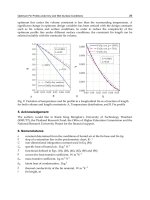
(i.e. yn ) involves evaluating the function g(x,y) all about the solution point xn, yn (see Figure 5.1).
By setting equations (5.1.19) and (5.1.20) equal to each other, we see that we can write the solution
in the from
yn+1 = yn + α0t0 + α1t1 + " + αktk ,

(5.1.21)
where the tis can be expressed recursively by

t 0 = hg ( x n , y n )



t 1 = hg[( x n + µ1 h ), ( y n + λ 1, 0 t 0 )]


t 2 = hg[( x n + µ 2 h ), ( y n + λ 2,0 t 0 + λ 2,1 t 1 )]
 .

#
#

t k = hg[( x n + µ k h ), ( y n + λ k ,0 t 0 + λ k ,1 t 1 + " + λ k ,k −1 t k −1 )] 

126

(5.1.22)


5 @ Differential and Integral Equations
Now we must determine k+1 values of α, k values of µ and k×(k+1)/2 values of λi,j. But we only have k+1
terms of the Taylor series to act as constraints. Thus, the problem is hopelessly under-determined. Thus
indeterminency will give rise to entire families of Runge-Kutta formulae for any order k. In addition, the
algebra to eliminate as many of the unknowns as possible is quite formidable and not unique due to the
undetermined nature of the problem. Thus we will content ourselves with dealing only with low order
formulae which demonstrate the basic approach and nature of the problem. Let us consider the lowest order

that provides some insight into the general aspects of the Runge-Kutta method. That is k=1. With k=1
equations (5.1.21) and (5.1.22) become

y n +1 = y n + α 0 t 0 + α 1 t 1



t 0 = hg ( x n y n )
 .
t 1 = hg[( x n + µh ), ( y n + λt 0 )] 

(5.1.23)

Here we have dropped the subscript on λ as there will only be one of them. However, there are still four free
parameters and we really only have three equations of constraint.

Figure 5.1 show the solution space for the differential equation
y' = g(x,y). Since the initial value is different for different solutions, the
space surrounding the solution of choice can be viewed as being full of
alternate solutions. The two dimensional Taylor expansion of the RungeKutta method explores this solution space to obtain a higher order value
for the specific solution in just one step.

127


Numerical Methods and Data Analysis
If we expand g(x,y) about xn, yn, in a two dimensional taylor series, we can write

g[( x n + µh ), ( y n + λt 0 )] = g ( x n , y n ) + µh
+ 12 λ2 t 02

∂g( x n , y n )
∂g( x n , y n ) 1 2 2 ∂g( x n , y n )
+ λt 0
+ 2µ h
∂x
∂y
∂x 2

∂ 2 g(x n , y n )
∂ 2 g(x n , y n )
+
µλ
t
+"+
0
∂x∂y
∂y 2

.

(5.1.24)

.

(5.1.25)

Making use of the third of equations (5.1.23), we can explicitly write t1 as

 ∂g( x n , y n )

∂g( x n , y n ) 
t 1 = hg( x n , y n ) + h 2 µ
+ λg ( x n , y n )

∂x
∂y


2
2
 2 ∂ g( x n , y n )
∂ g( x n , y n )
∂ 2 g( x n , y n ) 
2 2
1 3
+ λ g (x n , y n )
+ 2µλg( x n , y n )

2 h µ
∂x∂y 
∂x 2
∂y 2

Direct substitution into the first of equations (5.1.23) gives

 ∂g( x n , y n )
∂g( x n , y n ) 
y n +1 = y n + h (α 0 + α1 )g ( x n , y n ) + h 2 µ
+ λg ( x n , y n )


∂x
∂y


. (5.1.26)
2
2
2


g
(
x
,
y
)
g
(
x
,
y
)
g
(
x
,
y
)
∂
∂

∂
2
n
n
n
n
n
n
1 3
+ λ2 g 2 ( x n , y n )
+ 2µλg( x n , y n )

2 h α 1 µ
2
2
∂x∂y 
∂x
∂y

We can also expand y' in a two dimensional taylor series making use of the original differential equation
(5.1.3) to get

y ' = g ( x , y)
∂g( x , y)
∂g( x , y) ∂g ( x, y)
∂g ( x, y)
+ y'
=
+ g ( x , y)
y" =

∂x
∂y
∂x
∂y
y' ' ' =

∂y"
∂y" ∂ 2 g( x , y) ∂g ( x, y) ∂g( x, y)
∂ 2 g ( x , y)
+ y'
=
+
•
+
g
(
x
,
y
)
∂x
∂y
∂x
∂y
∂x∂y
∂x 2
2

 ∂g( x, y) 
∂ 2 g ( x , y)

∂ 2 g ( x , y)
+ g ( x , y)
+ g ( x , y) 
+
g
(
x
,
y
)

∂y∂x
∂y 2
 ∂y 






 .






(5.1.27)

Substituting this into the standard form of the Taylor series as given by equation (5.1.19) yields

 ∂g ( x , y)
∂ 2 g ( x , y) 
∂g ( x , y)  h 3  ∂ 2 g ( x , y)
2

y n +1 = y n + hg ( x , y) + h 2 
g
(
x
,
y
)
+
+
+ λg ( x , y)

∂y  6  ∂x 2
∂y 2 
 ∂x
 .
∂ 2 g ( x , y) ∂g ( x , y)  ∂g ( x , y)
∂g ( x , y)  


+ 2g ( x , y )
+
+ g ( x , y)





∂x∂y
∂y  ∂x
∂y  

(5.1.28)
Now by comparing this term by term with the expansion shown in equation (5.1.26) we can conclude that
the free parameters α0, α1, µ, and λ must be constrained by

128


5 @ Differential and Integral Equations

(α 0 + α 1 ) = 1 

α1µ = 12
 .

1
α1λ = 2


(5.1.29)

As we suggested earlier, the formula is under-determined by one constraint. However, we may use the
constraint equations as represented by equation (5.1.29) to express the free parameters in terms of a single
constant c. Thus the parameters are

α0 = 1− c



α1 = c
 .
1
µ = λ = 2 c 

(5.1.30)

and the approximation formula becomes

 ∂g ( x, y)
∂ 2 g ( x , y) 
∂g( x , y)  h 3  ∂ 2 g( x , y)
2
+
+
y n +1 = y n + hg( x , y) + h 2 
g
(
x
,
y
)
+ λg ( x , y)


∂y  8c  ∂x 2

∂y 2 
 ∂x
.
∂ 2 g ( x , y) 

+ 2g( x, y)


∂x∂y 

(5.1.31)
We can match the first two terms of the Taylor series with any choice of c. The error term will than be of
order O(h3) and specifically has the form

R n +1

∂g( x n , y n ) "
h3 
 [3 − 4c]y 'n'' − 3
=−
yn
∂y
24c 


 .


(5.1.32)

Clearly the most effective choice of c will depend on the solution so that there is no general "best" choice.
However, a number of authors recommend c = ½ as a general purpose value.
If we increase the number of terms in the series, the under-determination of the constants gets
rapidly worse. More and more parameters must be chosen arbitrarily. When these formulae are given, the
arbitrariness has often been removed by fiat. Thus one may find various Runge-Kutta formulae of the same
order. For example, a common such fourth order formula is

y n +1 = y n + ( t 0 + 2t 1 + 2t 2 + t 3 ) / 6
t 0 = hg( x n , y n )
t 1 = hg[( x n + 12 h ), ( y n + 12 t 0 )]
t 2 = hg[( x n + h ), ( y n + t )]
1
2

1
2 1

t 3 = hg[( x n + h ), ( y n + t 2 )]





 .




(5.1.33)

Here the "best" choice for the under-determined parameters has already been made largely on the basis of
experience.
If we apply these formulae to our test differential equation (5.1.10), we need first specify which
Runge-Kutta formula we plan to use. Let us try the second order (i.e. exact for quadratic polynomials)
formula given by equation (5.1.23) with the choice of constants given by equation (5.1.29) when c = ½. The

129


Numerical Methods and Data Analysis
formula then becomes

y n +1 = y n + 12 t 0 + 12 t 1



t 0 = hg ( x n , y n )
 .
t 1 = hg[( x n + h ), ( y n + t 0 )]

(5.1.34)

So that we may readily compare to the first order Picard formula, we will take h = 1 and y(0) = 1. Then
taking g(x,y) from equation (5.1.10) we get for the first step that

t 0 = hx 0 y 0 = (1)(0)(1) = 0



t 1 = h ( x 0 + h )( y 0 + t 0 ) = (1)(0 + 1)(1 + 0) = 1  .


y( x 0 + h ) = y1 = (1) + ( 1 2 )(0) + ( 1 2 )(1) = 32


(5.1.35)

The second step yields

t 0 = hx 1 y1 = (1)(1)( 3 2 ) =



t 1 = h ( x 1 + h )( y1 + t 0 ) = (1)(1 + 1)(1 + 3 2 ) = 5  .
y( x 1 + h ) = y 2 = ( 3 2 ) + ( 1 2 )( 3 2 ) + ( 1 2 )(5) = 194 
3
2

(5.1.36)

Table 5.2
Sample Runge-Kutta Solutions
Second Order Solution
i
0
1
2
3
y1
δy1

Fourth Order Solution
Step 1
h=1/2
ti
[0 , 9/32]
[1/4 , 45/64]
---------------------

h=1
ti
0.0
1.0
--------------------1.5

1.6172

h=1
ti
0.00000
0.50000
0.62500
1.62500

1.64587

1.65583

0.1172
0.8532*

h '1
i
0
1
2
3

ti
1.5
5.0
---------------------

Step 2
ti
[0.8086 , 2.1984]
[1.8193 , 5.1296]
---------------------

y2
δy2

4.75

6.5951

1.8451
h'2
0.0635
* This value assumes that δy0 = 0.1

130

yc

ti
1.64583
3.70313
5.24609
13.78384
7.38906

7.20051


5 @ Differential and Integral Equations
The Runge-Kutta formula tends to under-estimate the solution in a systematic fashion. If we reduce the step
size to h = ½ the agreement is much better as the error term in this formula is of O(h3). The results for
h=
½ are given in table 5.2 along with the results for h = 1. In addition we have tabulated the results for the
fourth order formula given by equation (5.1.33) For our example, the first step would require that equation
(5.1.33) take the form

t 0 = hx 0 y 0 = (1)(0)(1) = 0
t 1 = h ( x 0 + h )( y 0 + t 0 ) = (1)(0 + 2 )(1 + 0) =
1
2

1
2

1

1
2

t 2 = h ( x 0 + 12 h )( y 0 + 12 t 1 ) = (1)(0 + 1 2 )[1 + ( 1 2 )( 1 2 )] =

5
8

t 3 = h ( x 0 + 12 h )( y 0 + 12 t 2 ) = (1)(0 + 1)[1 + ( 1 2 )( 5 8 )] = 138
y( x 0 + h ) = y1 = (1) + [(0) + 2( 1 2 ) + 2( 5 8 ) + (13 8 )] / 6) =

79
48





 .




(5.1.37)

The error term for this formula is of O(h5) so we would expect it to be superior to the second order formula
for h = ½ and indeed it is. These results demonstrate that usually it is preferable to increase the accuracy of a
solution by increasing the accuracy of the integration formula rather than decreasing the step size. The

calculations leading to Table 5.2 were largely carried out using fractional arithmetic so as to eliminate the
round-off error. The effects of round-off error are usually such that they are more serious for a diminished
step size than for an integration formula yielding suitably increased accuracy to match the decreased step
size. This simply accentuates the necessity to improve solution accuracy by improving the approximation
accuracy of the integration formula.
The Runge-Kutta type schemes enjoy great popularity as their application is quite straight forward
and they tend to be quite stable. Their greatest appeal comes from the fact that they are one-step methods.
Only the information about the function at the previous step is necessary to predict the solution at the next
step. Thus they are extremely useful in initiating a solution starting with the initial value at the boundary of
the range. The greatest drawback of the methods is their relative efficiency. For example, the forth order
scheme requires four evaluations of the function at each step. We shall see that there are other methods that
require far fewer evaluations of the function at each step and yet have a higher order.

b.

Error Estimate and Step Size Control

A numerical solution to a differential equation is of little use if there is no estimate of its
accuracy. However, as is clear from equation (5.1.32), the formal estimate of the truncation error is often
more difficult than finding the solution. Unfortunately, the truncation error for most problems involving
differential equations tends to mimic the solution. That is, should the solution be monotonically increasing,
then the absolute truncation error will also increase. Even monotonically decreasing solutions will tend to
have truncation errors that keep the same sign and accumulate as the solution progresses. The common effect
of truncation errors on oscillatory solutions is to introduce a "phase shift" in the solution. Since the effect of
truncation error tends to be systematic, there must be some method for estimating its magnitude.

131


Numerical Methods and Data Analysis

Although the formal expression of the truncation error [say equation (5.1.32)] is usually rather
formidable, such expressions always depend on the step size. Thus we may use the step size h itself to
estimate the magnitude of the error. We can then use this estimate and an a priori value of the largest
acceptable error to adjust the step size. Virtually all general algorithms for the solution of differential
equations contain a section for the estimate of the truncation error and the subsequent adjustment of the step
size h so that predetermined tolerances can be met. Unfortunately, these methods of error estimate will rely
on the variation of the step size at each step. This will generally triple the amount of time required to effect
the solution. However, the increase in time spent making a single step may be offset by being able to use
much larger steps resulting in an over all savings in time. The general accuracy cannot be arbitrarily
increased by decreasing the step size. While this will reduce the truncation error, it will increase the effects
of round-off error due to the increased amount of calculation required to cover the same range. Thus one
does not want to set the a priori error tolerance to low or the round-off error may destroy the validity of the
solution. Ideally, then, we would like our solution to proceed with rather large step sizes (i.e. values of h)
when the solution is slowly varying and automatically decrease the step size when the solution begins to
change rapidly. With this in mind, let us see how we may control the step size from tolerances set on the
truncation error.
Given either the one step methods discussed above or the multi-step methods that follow, assume
that we have determined the solution yn at some point xn. We are about to take the next step in the solution to
xn+1 by an amount h and wish to estimate the truncation error in yn+1. Calculate this value of the solution two
ways. First, arriving at xn+1 by taking a single step h, then repeat the calculation taking two steps of (h/2). Let
us call the first solution y1,n+1 and the second y2,n+1. Now the exact solution (neglecting earlier accumulated
error) at xn+1 could be written in each case as

y e = y1,n +1 + αh k +1 + " +
y e = y 2,n +1 + 2α( 1 2 h k +1 ) + " +


 ,


(5.1.38)

where k is the order of the approximation scheme. Now α can be regarded as a constant throughout the
interval h since it is just the coefficient of the Taylor series fit for the (k+1)th term. Now let us define δ as a
measure of the error so that
δ(yn+1)  y2,n+1 ─ y1,n+1 = αhk+1/(1-2k) .
(5.1.39)
Clearly,
δ(yn+1) ~ hk+1 ,
(5.1.40)
so that the step size h can be adjusted at each step in order that the truncation error remains uniform by
hn+1 = hn│δ(yn)/δ(yn+1)│k+1 .
(5.1.41)
Initially, one must set the tolerance at some pre-assigned level ε so that
│δy0│ ε .

(5.1.42)

If we use this procedure to investigate the step sizes used in our test of the Runge-Kutta method, we
see that we certainly chose the step size to be too large. We can verify this with the second order solution for
we carried out the calculation for step sizes of h=1 and h=½. Following the prescription of equation (5.1.39)
and (5.1.41) we have, that for the results specified in Table 5.2,

132


5 @ Differential and Integral Equations

δy1 = y 2, 2 − y1,1 = 1.6172 − 1.500 = 0.1172
h1 = h 0

δy 0

δy1

= (1)(0.1 / 0.1172) = 0.8532



 .



(5.1.43)

Here we have tacitly assumed an initial tolerance of δy0 = 0.1. While this is arbitrary and rather large for a
tolerance on a solution, it is illustrative and consistent with the spirit of the solution. We see that to maintain
the accuracy of the solution within │0.1│ we should decrease the step size slightly for the initial step. The
error at the end of the first step is 0.16 for h = 1, while it is only about 0.04 for h = ½. By comparing the
numerical answers with the analytic answer, yc, we see that factor of two change in the step size reduces the
error by about a factor of four. Our stated tolerance of 0.1 requires only a reduction in the error of about 33%
which implies a reduction of about 16% in the step size or a new step size h1' = 0.84h1. This is amazingly
close to the recommended change, which was determined without knowledge of the analytic solution.
The amount of the step size adjustment at the second step is made to maintain the accuracy that
exists at the end of the first step. Thus,

δy 2 = y 2, 2 − y1, 2 = 6.5951 − 4.7500 = 1.8451




 .
y
δ
1
h 2 = h1
= (1)(0.1172 / 1.8451) = 0.0635 
δy 2


(5.1.44)

Normally these adjustments would be made cumulatively in order to maintain the initial tolerance. However,
the convenient values for the step sizes were useful for the earlier comparisons of integration methods. The
rapid increase of the solution after x = 1 causes the Runge-Kutta method to have an increasingly difficult
time maintaining accuracy. This is abundantly clear in the drastic reduction in the step size suggested at the
end of the second step. At the end of the first step, the relative errors where 9% and 2% for the h=1 and h=½
step size solutions respectively. At the end of the second step those errors, resulting from comparison with
the analytic solution, had jumped to 55% and 12% respectively (see table 5.2). While a factor of two-change
in the step size still produces about a factor of four change in the solution, to arrive at a relative error of 9%,
we will need more like a factor of 6 change in the solution. This would suggest a change in the step size of a
about a factor of three, but the recommended change is more like a factor of 16. This difference can be
understood by noticing that equation (5.1.42) attempts to maintain the absolute error less than δyn. For our
problem this is about 0.11 at the end of step one. To keep the error within those tolerances, the accuracy at
step two would have to be within about 1.5% of the correct answer. To get there from 55% means a
reduction in the error of a factor of 36, which corresponds to a reduction in the step size of a factor of about
18, is close to that given by the estimate.
Thus we see that the equation (5.1.42) is designed to maintain an absolute accuracy in the solution
by adjusting the step size. Should one wish to adjust the step size so as to maintain a relative or percentage
accuracy, then one could adjust the step size according to
hn+1 = hn│{[δ(yn)yn+1]/[δ(yn+1)yn]}│k+1 .

(5.1.45)

While these procedures vary the step size so as to maintain constant truncation error, a significant price in
the amount of computing must be paid at each step. However, the amount of extra effort need not be used
only to estimate the error and thereby control it. One can solve equations (5.1.38) (neglecting terms of order
greater than k) to provide an improved estimate of yn+1. Specifically

133


Numerical Methods and Data Analysis
ye ≅ y2,n+1 + δ(yn+1)/(2k-1) .

(5.1.46)

However, since one cannot simultaneously include this improvement directly in the error estimate, it is
advisable that it be regarded as a "safety factor" and proceeds with the error estimate as if the improvement
had not been made. While this may seem unduly conservative, in the numerical solution of differential
equations conservatism is a virtue.

c.

Multi-Step and Predictor-Corrector Methods

The high order one step methods achieve their accuracy by exploring the solution space in
the neighborhood of the specific solution. In principle, we could use prior information about the solution to
constrain our extrapolation to the next step. Since this information is the direct result of prior calculation, far
greater levels of efficiency can be achieved than by methods such as Runge-Kutta that explore the solution
space in the vicinity of the required solution. By using the solution at n points we could, in principle, fit an

(n-1) degree polynomial to the solution at those points and use it to obtain the solution at the (n+1)st point.
Such methods are called multi-step methods. However, one should remember the caveats at the end of
chapter 3 where we pointed out that polynomial extrapolation is extremely unstable. Thus such a procedure
by itself will generally not provide a suitable method for the solution of differential equations. But when
combined with algorithms that compensate for the instability such schemes can provide very stable solution
algorithms. Algorithms of this type are called predictor-corrector methods and there are numerous forms of
them. So rather than attempt to cover them all, we shall say a few things about the general theory of such
schemes and give some examples.
A predictor-corrector algorithm, as the name implies, consists of basically two parts. The predictor
extrapolates the solution over some finite range h based on the information at prior points and is inherently
unstable. The corrector allows for this local instability and makes a correction to the solution at the end of
the interval also based on prior information as well as the extrapolated solution. Conceptually, the notion of a
predictor is quite simple. In its simplest form, such a scheme is the one-step predictor where
yn+1 = yn + hy'n .
(5.1.47)
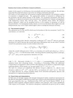
By using the value of the derivative at xn the scheme will systematically under estimate the proper
value required for extrapolation of any monotonically increasing solution (see figure 5.2). The error will
build up cumulatively and hence it is unstable. A better strategy would be to use the value of the derivative
midway between the two solution points, or alternatively to use the information from the prior two points to
predict yn+1. Thus a two point predictor could take the form
(5.1.48)
yn+1 = yn-1 +2hy'n .
Although this is a two-point scheme, the extrapolating polynomial is still a straight line. We could
have used the value of yn directly to fit a parabola through the two points, but we didn't due to the
instabilities to be associated with a higher degree polynomial extrapolation. This deliberate rejection of the
some of the informational constraints in favor of increased stability is what makes predictor-corrector
schemes non-trivial and effective. In the general case, we have great freedom to use the information we have
regarding yi and y'
i. If we were to include all the available information, a general predictor would have the
form

n
n

134


5 @ Differential and Integral Equations
yn+1 = Σ aiyi + h Σ biy'i + R ,
i=0

i=0

(5.1.49)

where the ai s and bi s are chosen by imposing the appropriate constraints at the points xi and R is an error
term.
When we have decided on the form of the predictor, we must implement some sort of corrector
scheme to reduce the truncation error introduced by the predictor. As with the predictor, let us take a simple
case of a corrector as an example. Having produced a solution at xn+1 we can calculate the value of the
derivative y'n+1 at xn+1. This represents new information and can be used to modify the results of the
prediction. For example, we could write a corrector as
(k-1)
y(k)
n+1= yn + ½h[y' n+1 + y'n ] .

(5.1.50)

Therefore, if we were to write a general expression for a corrector based on the available information we
would get

Figure 5.2 shows the instability of a simple predictor scheme that systematically
underestimates the solution leading to a cumulative build up of truncation error.
n

n

i =0

i =0

y (nk+)1 = ∑ α i y i + h ∑ β i y'i + hβ n +1 y' n(+k1+1) .

(5.1.51)

Equations (5.1.50) and (5.1.51) both are written in the form of iteration formulae, but it is not at all clear that

135


Numerical Methods and Data Analysis
the fixed-point for these formulae is any better representation of the solution than single iteration. So in order
to minimize the computational demands of the method, correctors are generally applied only once. Let us
now consider certain specific types of predictor corrector schemes that have been found to be successful.
Hamming1 gives a number of popular predictor-corrector schemes, the best known of which is the
Adams-Bashforth-Moulton Predictor-Corrector. Predictor schemes of the Adams-Bashforth type emphasize
the information contained in prior values of the derivative as opposed to the function itself. This is
presumably because the derivative is usually a more slowly varying function than the solution and so can be
more accurately extrapolated. This philosophy is carried over to the Adams-Moulton Corrector. A classical
fourth-order formula of this type is

y (n1+)1 = y n + h (55 y 'n − 59 y 'n −1 + 37 y 'n − 2 − 9 y 'n −3 ) / 24
y n +1 = y n + h (9 y 'n +1 + 19 y 'n − 5y 'n −1 ) / 24

+ O( h 5 )

+ O( h 5 )


 .


(5.1.52)

Lengthy study of predictor-corrector schemes has evolved some special forms such as this one

z n +1 = (2 y n −1 + y n − 2 ) / 3 + h (191y 'n − 107 y 'n −1 + 109 y 'n − 2 − 25y 'n −3 ) / 75 

u n +1 = z n +1 − 707(z n − c n ) / 750

 . (5.1.53)
c n +1 = (2 y n −1 + y n − 2 ) / 3 + h (25u ' n +1 +91y' n +43y' n −1 +9 y' n − 2 ) / 72

6

y n +1 = c n +1 + 43(z n +1 − c n +1 ) / 750 + O(h )

where the extrapolation formula has been expressed in terms of some recursive parameters ui and ci. The
derivative of these intermediate parameters are obtained by using the original differential equation so that
u' = g(x,u) .

(5.1.54)

By good chance, this formula [equation (5.1.53)] has an error term that varies as O(h6) and so is a fifth-order
formula. Finally a classical predictor-corrector scheme which combines Adams-Bashforth and Milne
predictors and is quite stable is parametrically ( i.e. Hamming p206)

z n +1 = 12 ( y n + y n −1 ) + h (119 y 'n − 99 y 'n −1 + 69 y 'n − 2 − 17 y 'n −3 ) / 48
u n +1 = z n +1 − 161(z n − c n ) / 170
c n +1 = 12 ( y n + y n −1 ) + h (17 u ' n +1 +51y' n +3y' n −1 + y' n − 2 ) / 48
y n +1 = c n +1 + 9(z n +1 − c n +1 ) / 170 + O(h 6 )




.




(5.1.55)

Press et al2 are of the opinion that predictor-corrector schemes have seen their day and are made
obsolete by the Bulirsch-Stoer method which they discuss at some length3. They quite properly point out that
the predictor-corrector schemes are somewhat inflexible when it comes to varying the step size. The step size
can be reduced by interpolating the necessary missing information from earlier steps and it can be expanded
in integral multiples by skipping earlier points and taking the required information from even earlier in the
solution. However, the Bulirsch-Stoer method, as described by Press et. al. utilizes a predictor scheme with
some special properties. It may be parameterized as

136

5 @ Differential and Integral Equations



z 1 = z 0 + hz' 0


z k +1 = z k −1 + hz' k k = 1,2,3,", n − 1  .

y (n1) = 1 2 (z n + z n −1 + hz' n ) + O(h 5 ) 

z ' = g ( z, x )
z 0 = y( x 0 )

(5.1.56)

It is an odd characteristic of the third of equations (5.1.56) that the error term only contains even
powers of the step size. Thus, we may use the same trick that was used in equation (5.1.46) of utilizing the
information generated in estimating the error term to improve the approximation order. But since only even
powers of h appear in the error term, this single step will gain us two powers of h resulting in a predictor of
order seven.
(1)
7
ynh = {4y(1)
(5.1.57)
n (x+nh) ─ yn/2 [x+(n/2)(2h)]}/3 + O(h ) .
This yields a predictor that requires something on the order of 1½ evaluations of the function per step
compared to four for a Runge-Kutta formula of inferior order.

Now we come to the aspect of the Bulirsch-Stoer method that begins to differentiate it from classical
predictor-correctors. A predictor that operates over some finite interval can use a successively increasing
number of steps in order to make its prediction. Presumably the prediction will get better and better as the
step size decreases so that the number of steps to make the one prediction increases. Of course practical
aspects of the problem such as roundoff error and finite computing resources prevent us from using
arbitrarily small step sizes, but we can approximate what would happen in an ideal world without round-off
error and utilizing unlimited computers. Simply consider the prediction at the end of the finite interval H
where
H = αh .
(5.1.58)
Thus yα(x+H) can be taken to be a function of the step size h so that,
yα(x+H) = y(x+αh) = f(h) .

(5.1.59)

Now we can phrase our problem to estimate the value of that function in the limit
Lim f(h) = Y∞(x+H) .
h→0
α→∞

(5.1.60)

We can accomplish this by carrying out the calculation for successively smaller and smaller values of h and,
on the basis of these values, extrapolating the result to h=0. In spite of the admonitions raised in chapter 3
regarding extrapolation, the range here is small. But to produce a truly powerful numerical integration
algorithm, Bulirsch and Stoer carry out the extrapolation using rational functions in the manner described in
section 3.2 [equation (3.2.65)]. The superiority of rational functions to polynomials in representing most
analytic functions means that the step size can be quite large indeed and the conventional meaning of the
'order' of the approximation is irrelevant in describing the accuracy of the method.

137


Numerical Methods and Data Analysis
In any case, remember that accuracy and order are not synonymous! Should the solution be
described by a slowly varying function and the numerical integration scheme operate by fitting high order
polynomials to prior information for the purposes of extrapolation, the high-order formula can give very
inaccurate results. This simply says that the integration scheme can be unstable even for well behaved
solutions.
Press et. al.4 suggest that all one needs to solve ordinary differential equations is either a RungeKutta or Bulirsch-Stoer method and it would seem that for most problems that may well be the case.
However, there are a large number of commercial differential equation solving algorithms and the majority
of them utilize predictor-corrector schemes. These schemes are generally very fast and the more
sophisticated ones carry out very involved error checking algorithms. They are generally quite stable and can
involve a very high order when required. In any event, the user should know how they work and be wary of
the results. It is far too easy to simply take the results of such programs at face value without ever
questioning the accuracy of the results. Certainly one should always ask the question "Are these results
reasonable?" at the end of a numerical integration. If one is genuinely skeptical, it is not a bad idea to take
the final value of the calculation as an initial value and integrate back over the range. Should one recover the
original initial value within the acceptable tolerances, one can be reasonably confident that the results are
accurate. If not, the difference between the beginning initial value and what is calculated by the reverse
integration over the range can be used to place limits on the accuracy of the initial integration.

d.

Systems of Differential Equations and Boundary Value Problems

All the methods we have developed for the solution of single first order differential
equations may be applied to the case where we have a coupled system of differential equations. We saw
earlier that such systems arose whenever we dealt with ordinary differential equations of order greater than
one. However, there are many scientific problems which are intrinsically described by coupled systems of

differential equations and so we should say something about their solution. The simplest way to see the
applicability of the single equation algorithms to a system of differential equations is to write a system like

y'1 = g 1 ( x , y1 , y 2 ," y n ) 
y' 2 = g 2 ( x , y1 , y 2 , " y n ) 
 ,
#
#

y' n = g n ( x , y1 , y 2 , " y n )

(5.1.61)

as a vector where each element represents one of the dependent variables or unknowns of the system. Then
the system becomes
G G G
y ' = g ( x , y) ,
(5.1.62)
which looks just like equation (5.1.3) so that everything applicable to that equation will apply to the system
of equations. Of course some care must be taken with the terminology. For example, equation (5.1.4) would
have to be understood as standing for an entire system of equations involving far more complicated integrals,
but in principle, the ideas carry over. Some care must also be extended to the error analysis in that the error

G

term is also a vector R (x). In general, one should worry about the magnitude of the error vector, but in

138

5 @ Differential and Integral Equations
practice, it is usually the largest element that is taken as characterizing the accuracy of the solution.
To generate a numerical integration method for a specific algorithm, one simply applies it to each of
the equations that make up the system. By way of a specific example, let's consider a forth order RungeKutta algorithm as given by equation (5.1.33) and apply it to a system of two equations. We get

y1,n +1 = y1,n + ( t 0 + 2 t 1 + 2 t 2 + t 3 ) / 6



y 2,n +1 = y 2,n + (u 0 + 2u 1 + 2u 2 + u 3 ) / 6


t 0 = hg 1 ( x n , y1,n , y 2,n )

t 1 = hg 1 [( x n + 1 2 h ), ( y1,n + 1 2 t 0 ), ( y 2,n + 1 2 u 0 )] 

t 2 = hg 1 [( x n + 1 2 h ), ( y1,n + 1 2 t 1 ), ( y 2,n + 1 2 u 1 )] 
 .
t 3 = hg 1 [( x n + h ), ( y1,n + t t ), ( y 2,n + u 2 )]


u 0 = hg 2 ( x n , y1,n , y 2,n )

u 1 = hg 2 [( x n + 1 2 h ), ( y1,n + 1 2 t 0 ), ( y 2,n + 1 2 u 0 )] 

u 2 = hg 2 [( x n + 1 2 h ), ( y1,n + 1 2 t 1 ), ( y 2,n + 1 2 u 1 )] 

u 1 = hg 2 [( x n + h ), ( y1,n + t t ), ( y 2,n + u 2 )]


(5.1.63)

We can generalize equation (5.1.63) to an arbitrary system of equations by writing it in vector form as

G G
G
y n +1 = A( y n ) .

(5.1.64)

G G
The vector A ( y n ) consists of elements which are functions of dependent variables yi,n and xn, but which all
G
have the same general form varying only with gi(x, y ). Since an nth order differential equation can always
be reduced to a system of n first order differential equations, an expression of the form of equation (5.1.63)
could be used to solve a second order differential equation.
The existence of coupled systems of differential equations admits the interesting possibility that the
constants of integration required to uniquely specify a solution are not all given at the same location. Thus
we do not have a full compliment of yi,0's with which to begin the integration. Such problems are called
boundary value problems. A comprehensive discussion of boundary value problems is well beyond the
scope of this book, but we will examine the simpler problem of linear two point boundary value problems.
This subclass of boundary value problems is quite common in science and extremely well studied. It consists
of a system of linear differential equations (i.e. differential equations of the first degree only) where part of
the integration constants are specified at one location x0 and the remainder are specified at some other value
of the independent variable xn. These points are known as the boundaries of the problem and we seek a
solution to the problem within these boundaries. Clearly the solution can be extended beyond the boundaries
as the solution at the boundaries can serve as initial values for a standard numerical integration.
The general approach to such problems is to take advantage of the linearity of the equations, which
guarantees that any solution to the system can be expressed as a linear combination of a set of basis

139


Numerical Methods and Data Analysis
solutions. A set of basis solutions is simply a set of solutions, which are linearly independent. Let us consider
a set of m linear first order differential equations where k values of the dependent variables are specified at
x0 and (m-k) values corresponding to the remaining dependent variables are specified at xn. We could solve
(m-k) initial value problems starting at x0 and specifying (m-k) independent, sets of missing initial values so
that the initial value problems are uniquely determined. Let us denote the missing set of initial values at x0 by
G
y ( 0) ( x 0 ) which we know can be determined from initial sets of linearly independent trial initial values
j

G
y ( t ) ( x 0 ) by

G
y ( 0 ) ( x 0 ) = Ay ( t ) ( x 0 ) ,
(5.1.65)
j G (t)
(t)
The columns of y (x0) are just the individual vectors y ( x 0 ) . Clearly the matrix A will have to be
G
diagonal to always produce y ( 0 ) ( x 0 ) . Since the trial initial values are arbitrary, we will choose the elements
of the (m-k) sets to be

j

yi(x0) = δij ,

so that the missing initial values will be

(5.1.66)

G
y ( 0 ) ( x 0 ) 1 = 1A = A .

(5.1.67)

G

Integrating across the interval with these initial values will yield (m-k) solution j y ( t ) ( x n ) at the
other boundary. Since the equations are linear each trial solution will be related to the known boundary
G
values j y ( t ) ( x n ) by

G
G
y ( 0 ) ( x n ) = A[ j y ( t ) ( x n )] ,

(5.1.68)

so that for the complete set of trial solutions we may write

G
y ( 0) ( x n ) 1 = Ay(t)(xn) ,

(5.1.69)

G

where by analogy to equation (5.1.65), the column vectors of y(t)(xn) are j y ( t ) ( x n ) . We may solve these
equations for the unknown transformation matrix A so that the missing initial values are

G
G
y ( 0) ( x n ) 1 = A = y-1 y ( 0) ( x n ) .

(5.1.70)

If one employs a one step method such as Runge-Kutta, it is possible to collapse this entire operation to the
point where one can represent the complete boundary conditions at one boundary in terms of the values at
G
the other boundary y n a system of linear algebraic equations such as

G
G
y ( x 0 ) = By ( x n ) .

5.1.71)

The matrix B will depend only on the details of the integration scheme and the functional form of the
equations themselves, not on the boundary values. Therefore it may be calculated for any set of boundary
values and used repeatedly for problems differing only in the values at the boundary (see Day and Collins5).
To demonstrate methods of solution for systems of differential equations or boundary value

140


5 @ Differential and Integral Equations

problems, we shall need more than the first order equation (5.1.10) that we used for earlier examples.
However, that equation was quite illustrative as it had a rapidly increasing solution that emphasized the
shortcomings of the various numerical methods. Thus we shall keep the solution, but change the equation.
Simply differentiate equation (5.1.10) so that
x2
Y" = 2(1+2x2)e = 2(1+x2)y .
(5.1.72)
Let us keep the same initial condition given by equation (5.1.11) and add a condition of the derivative at
= 1 so that

y(0) = 1
y' (1) = 2e = 5.43656


 .


x

(5.1.73)

This insures that the closed form solution is the same as equation (5.1.12) so that we will be able to compare
the results of solving this problem with earlier methods. We should not expect the solution to be as accurate
for we have made the problem more difficult by increasing the order of the differential equation in addition
to separating the location of the constants of integration. This is no longer an initial value problem since the
solution value is given at x = 0, while the other constraint on the derivative is specified at x = 1. This is
typical of the classical two-point boundary value problem.
We may also use this example to indicate the method for solving higher order differential equations
given at the start of this chapter by equations (5.1.1) and (5.1.2). With those equations in mind, let us replace
equation (5.1.72) by system of first order equations

y'1 ( x ) = y 2 ( x )
y' 2 ( x ) = 2(1 + 2 x ) y1 ( x )
2

which we can write in vector form as

G
G
y' = A ( x ) y ,


 ,


(5.1.74)

(5.1.75)

where

0
1

A( x ) = 
2
 2(1 + x ) 0


 .




(5.1.76)

G

The components of the solution vector y are just the solution we seek (i.e.) and its derivative. However, the
form of equation (5.1.75) emphasizes its linear form and were it a scalar equation, we should know how to
proceed.
For purposes of illustration, let us apply the fourth order Runge-Kutta scheme given by equation
(5.1.63). Here we can take specific advantage of the linear nature of our problem and the fact that the
dependence on the independent variable factors out of the right hand side. To illustrate the utility of this fact,
let
g(x,y) = [f(x)]y ,
(5.1.77)
in equation (5.1.63).
Then we can write the fourth order Runge-Kutta parameters as

141


Numerical Methods and Data Analysis

t 0 = hf 0 y n
t 1 = hf1 ( y n + 1 2 t 0 ) = hf1 ( y n + 1 2 hf 0 y n = (hf1 + 1 2 h f 1f 0 ) y n
2

t 2 = hf1 ( y n + 1 2 t 1 ) = (hf1 + 1 2 h 2 f 12 + 1 4 h 3 f12 f 0 ) y n
t 3 = hf 2 ( y n + t 2 ) = (hf 2 + h 2 f 2 f1 + 1 2 h 3 f 12 f 2 + 1 4 h 4 f 2 f 12 f 0 ) y n




 .




(5.1.78)

where

f 0 = f (x n )
f1 = f ( x n +

1

2

h)

f 2 = f (x n + h)



 ,



(5.1.79)

so that the formula becomes

y n +1 = y n + ( t 0 + 2 t 1 2 t 2 + t 3 )
. (5.1.80)

 h
h2
h3 2
h4
(f 1f 0 + f 12 + f 2 f 1 ) +
(f 1 f 0 + f 2 f 12 ) +
f 2 f 12 f 0 ) y n
= 1 + (f 0 + 4f 1 + f 2 ) +
6
12
24

 6

Here we see that the linearity of the differential equation allows the solution at step n to be factored out of
the formula so that the solution at step n appears explicitly in the formula. Indeed, equation (5.1.80)
represents a power series in h for the solution at step (n+1) in terms of the solution at step n. Since we have
been careful about the order in which the functions fi multiplied each other, we may apply equation (5.1.80)
directly to equation (5.1.75) and obtain a similar formula for systems of linear first order differential
equations that has the form

 h
G

G
h2
h3 2
h4
2
2
y n +1 = 1 + (A 0 + 4A1 + A 2 ) + (A 0 A1 + 4A1 + A 2 A1 ) + (A1 A 0 + A 2 A1 ) + A 2 A12 A 0  y n .
6
12
24
 6

(5.1.81)
Here the meaning of Ai is the same as fi in that the subscript indicates the value of the independent variable x
for which the matrix is to be evaluated. If we take h = 1, the matrices for our specific problem become

1 

0  
1  
 .
0  
 0 1 

A 2 = 
 4 0 
 0
A 0 = 
 2
 0

A 1 = 
3

(5.1.82)

Keeping in mind that the order of matrix multiplication is important, the products appearing in the second
order term are

142


5 @ Differential and Integral Equations

 2
A 1 A 0 = 
 0
3
A 12 = 
 0




0

3 
 3 0

A 2 A 1 = 
 0 6

0
3





 .





(5.1.83)

The two products appearing in the third order term can be easily generated from equations (5.1.82) and
(5.1.83) and are

 0 3

A 12 A 0 = 
9 0
 0 3

A 2 A 12 = 
 18 0 





 .




(5.1.84)

Finally the single matrix of the first order term can be obtain by successive multiplication using
equations(5.1.82) and (5.1.84) yielding

0
9

A 2 A 12 A 0 = 
 0 18 


 .


(5.1.85)

Like equation (5.1.80), we can regard equation (5.1.81) as a series solution in h that yields a system of linear
equations for the solution at step n+1 in terms of the solution at step n. It is worth noting that the coefficients
of the various terms of order hk are similar to those developed for equal interval quadrature formulae in
chapter 4. For example the lead term being the unit matrix generates the coefficients of the trapezoid rule
while the h(+1, +4, +1)/6 coefficients of the second term are the familiar progression characteristic of
Simpson's rule. The higher order terms in the formula are less recognizable since they depend on the
parameters chosen in the under-determined Runge-Kutta formula.

If we define a matrix P(hk) so that

G
G
y n +1 = P(h k )≡ k P y n ,

(5.1.86)

the series nature of equation (5.1.81) can be explicitly represented in terms of the various values of kP.

For our problem they are:

143


Numerical Methods and Data Analysis

1 0

P = 
 0 1
1
1


1
P =  11
0 

6




 7
1

3
2

P=

 11
0


 6
3 
 7


3
2 
3

P=

 49
3 



 12
3
 65

24
2
4
P=
 49
15

4
 12
0


































 .




(5.1.87)

The boundary value problem now is reduced to solving the linear system of equations specified by equation
(5.1.86) where the known values at the respective boundaries are specified. Using the values given in
equation (5.1.73) the linear equations for the missing boundary values become

1= k P11 y1 (0)+ k P12 (5.43656)
y 2 (0)= P21 y1 (1)+ P22 (5.43656)

k

k


 .


(5.1.88)

The first of these yields the missing solution value at x = 0 [i.e. y2(0)]. With that value the remaining value
can be obtained from the second equation. The results of these solutions including additional terms of order
hk are given in table 5.3. We have taken h to be unity, which is unreasonably large, but it serves to
demonstrate the relative accuracy of including higher order terms and simplifies the arithmetic. The results
for the missing values y2(0) and y1(1) (i.e. the center two rows) converge slowly, and not uniformly, toward
their analytic values given in the column labeled k = ∞.
Had we chosen the step size h to be smaller so that a number of steps were required to cross the
interval, then each step would have produced a matrix kiP and the solution at each step would have been
related to the solution at the following step by equation (5.1.86). Repeated application of that equation would
yield the solution at one boundary in terms of the solution at the other so that

144


5 @ Differential and Integral Equations

G
y n =( n −k1 P

k

n −2

P

k
n −3

G
G
P "00 P ) y 0 = k Q y 0 .

(5.1.89)

Table 5.3
Solutions of a Sample Boundary Value Problem
for Various Orders of Approximation
\k
y1(0)
y2(0)
y1(1)
y2(1)

0
1.0
5.437
1.0
5.437

1
1.0

3.60
4.60
5.437

2
1.0
1.200
3.53
5.437

3
1.0
0.4510
3.01
5.437

∞
1.0
0.0
2.71828
2e

4
1.0
0.3609
3.25
5.437

Thus one arrives at a similar set of linear equations to those implied by equation (5.1.86) and explicitly given
in equation (5.1.88) relating the solution at one boundary in terms of the solution at the other boundary.

These can be solved for the missing boundary values in the same manner as our example. Clearly the
decrease in the step size will improve the accuracy as dramatically as increasing the order k of the
approximation formula. Indeed the step size can be variable at each step allowing for the use of the error
correcting procedures described in section 5.1b.

Table 5.4
Solutions of a Sample Boundary Value Problem
\k
y1(0)
y2(0)
y1(1)
y2(1)

0
1.0
0.0
1.0
0.0

1
1.0
0.0
1.0
1.83

2
1.0
0.0
2.33
1.83

3
1.0
0.0
2.33
4.08

4
1.0
0.0
2.708
4.08

∞
1.0
0.0
2.718
5.437

Any set of boundary values could have been used with equations (5.1.81) to yield the solution
elsewhere. Thus, we could treat our sample problem as an initial value problem for comparison. If we take
the analytic values for y1(0) and y2(0) and solve the resulting linear equations, we get the results given in
Table 5.4. Here the final solution is more accurate and exhibits a convergence sequence more like we would
expect from Runge-Kutta. Namely, the solution systematically lies below the rapidly increasing analytic
solution. For the boundary value problem, the reverse was true and the final result less accurate. This is not
an uncommon result for two-point boundary value problems since the error of the approximation scheme is
directly reflected in the determination of the missing boundary values. In an initial value problem, there is
assumed to be no error in the initial values.

145