Ebook Advanced engineering mathematics (7th edition) Part 2

PA R T

4
Fourier
Analysis,
Special
Functions,
and Eigenfunction
Expansions

CHAPTER 13
Fourier Series

CHAPTER 14
The Fourier Integral and
Transforms

CHAPTER 15
Special Functions and
Eigenfunction Expansions

Copyright 2010 Cengage Learning. All Rights Reserved. May not be copied, scanned, or duplicated, in whole or in part. Due to electronic rights, some third party content may be suppressed from the eBook and/or eChapter(s).
Editorial review has deemed that any suppressed content does not materially affect the overall learning experience. Cengage Learning reserves the right to remove additional content at any time if subsequent rights restrictions require it.

October 14, 2010

14:57

THM/NEIL

Page-425

27410_13_ch13_p425-464


CHAPTER

13

WHY FOURIER SERIES? THE FOURIER
SERIES OF A FUNCTION SINE AND
C O S I N E S E R I E S I N T E G R AT I O N A N D
D I F F E R E N T I AT I O N

Fourier Series

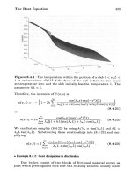
In 1807, Joseph Fourier submitted a paper to the French Academy of Sciences in competition for
a prize offered for the best mathematical treatment of heat conduction. In the course of this work
Fourier shocked his contemporaries by asserting that “arbitrary” functions (such as might specify
initial temperatures) could be expanded in series of sines and cosines. Consequences of Fourier’s
work have had an enormous impact on such diverse areas as engineering, music, medicine, and
the analysis of data.

13.1

Why Fourier Series?
A Fourier series is a representation of a function as a series of constant multiples of sine and/or
cosine functions of different frequencies. To see how such a series might arise, we will look at a
problem of the type that concerned Fourier.
Consider a thin homogeneous bar of metal of length π , constant density and uniform cross
section. Let u(x, t) be the temperature in the bar at time t in the cross section at x. Then (see

Section 12.8.2) u satisfies the heat equation
∂ 2u
∂u
=k 2
∂t
∂x
for 0 < x < π and t > 0. Here k is a constant depending on the material of the bar. If the left and
right ends are kept at temperature zero, then
u(0, t) = u(π, t) = 0 for t > 0.
These are the boundary conditions. Further, assume that the initial temperature has been
specified, say
u(x, 0) = f (x) = x(π − x).
This is the initial condition.
427

Copyright 2010 Cengage Learning. All Rights Reserved. May not be copied, scanned, or duplicated, in whole or in part. Due to electronic rights, some third party content may be suppressed from the eBook and/or eChapter(s).
Editorial review has deemed that any suppressed content does not materially affect the overall learning experience. Cengage Learning reserves the right to remove additional content at any time if subsequent rights restrictions require it.

October 14, 2010

14:57

THM/NEIL

Page-427

27410_13_ch13_p425-464


428

CHAPTER 13

Fourier Series

Fourier found that the functions
u n (x, t) = bn sin(nx)e−kn

2t

satisfy the heat equation and the boundary conditions, for every positive integer n and any number
bn . However, there is no choice of n and bn for which this function satisfies the initial condition,
which would require that
u n (x, 0) = bn sin(nx) = x(π − x).
for 0 ≤ x ≤ π.
We could try a finite sum of these functions, attempting a solution
N
2

bn sin(nx)e−kn t .

u(x, t) =
n=1

But this would require that N and numbers b1 , · · · , b N be found so that
N

u(x, 0) = x(π − x) =

bn sin(nx)

n=1

for 0 ≤ x ≤ π . Again, this is impossible. A finite sum of multiples of sine functions is not a
polynomial.
Fourier’s brilliant insight was to attempt an infinite superposition,
∞
2

bn sin(nx)e−kn t .

u(x, t) =
n=1

This function will still satisfy the heat equation and the boundary conditions u(x, 0) = u(π, 0) =
0. To satisfy the initial condition, the problem is to choose the numbers bn so that
∞

u(x, 0) = x(π − x) =

bn sin(nx)
n=1

for 0 ≤ x ≤ π . Fourier claimed not only that this could this be done, but that the right choice is
bn =

1
π

π

x(π − x) sin(nx) d x =

0

4 1 − (−1)n
.
π
n3

With these coefficients, Fourier wrote the solution for the temperature function:
4
u(x, t) =
π

∞

n=1

1 − (−1)n
2
sin(nx)e−kn t .
n3

The astonishing claim that
4
x(π − x) =
π

∞

n=1

1 − (−1)n
sin(nx)
n3

for 0 ≤ x ≤ π was too much for Fourier’s contemporaries to accept, and the absence of rigorous
proofs in his paper led the Academy to reject its publication (although they awarded him the
prize). However, the implications of Fourier’s work were not lost on natural philosophers of
his time. If Fourier was right, then many functions would have expansions as infinite series of
trigonometric functions.
Although Fourier did not have the means to supply the rigor his colleagues demanded, this
was provided throughout the ensuing century and Fourier’s ideas are now seen in many important
applications. We will use them to solve partial differential equations, beginning in Chapter 16.
This and the next two chapters develop the requisite ideas from Fourier analysis.

Copyright 2010 Cengage Learning. All Rights Reserved. May not be copied, scanned, or duplicated, in whole or in part. Due to electronic rights, some third party content may be suppressed from the eBook and/or eChapter(s).
Editorial review has deemed that any suppressed content does not materially affect the overall learning experience. Cengage Learning reserves the right to remove additional content at any time if subsequent rights restrictions require it.

October 14, 2010

14:57

THM/NEIL

Page-428

27410_13_ch13_p425-464

13.2 The Fourier Series of a Function

PROBLEMS

SECTION 13.1

2. Let p(x) be a polynomial. Prove that there is no number
k such that p(x) = k sin(nx) on [0, π ] for any positive
integer n.

1. Let
SN (x) =

4
π

N

1 − (−1)
sin(nx).
n3
n

n=1

3. Let p(x) be a polynomial. Prove that there is no finite
N
sum n=1 bn sin(nx) that is equal to p(x) for 0 ≤ x ≤ π ,
for any choice of the numbers b1 , · · · , b N .

Construct graphs of SN (x) and x(π − x), for 0 ≤ x ≤ π ,
for N = 2 and then N = 10. This will give some sense of
the correctness of Fourier’s claim that this polynomial
could be exactly represented by the infinite series
4
π

∞

n=1

429

1 − (−1)n
sin(nx)
n3

on [0, π ].

13.2

The Fourier Series of a Function
Let f (x) be defined on [−L , L]. We want to choose numbers a0 , a1 , a2 · · · and b1 , b2 , · · ·
so that
1
f (x) = a0 +
2

∞

[ak cos(kπ x/L) + bk sin(kπ x/L)].

(13.1)

k=1

This is a decomposition of the function into a sum of terms, each representing the influence of a
different fundamental frequency on the behavior of the function.
To determine a0 , integrate equation (13.1) term by term to get
L
−L

f (x)d x =

1
2

L

a0 d x
−L
∞

L

+

ak
−L

k=1

L

cos(kπ x/L) d x + bk

sin(kπ x/L) d x
−L

1
= a0 (2L) = πa0 .
2
because all of the integrals in the summation are zero. Then
a0 =

L

1
L

−L

f (x) d x.

(13.2)

To solve for the other coefficients in the proposed equation (13.1), we will use the following three
facts, which follow by routine integrations. Let m and n be integers. Then
L
−L

cos(nπ x/L) sin(mπ x/L) d x = 0.

(13.3)

Furthermore, if n = m, then
L
−L

L

cos(nπ x/L) cos(mπ x/L) d x =

−L

sin(nπ x/L) sin(mπ x/L) d x = 0.

(13.4)

Copyright 2010 Cengage Learning. All Rights Reserved. May not be copied, scanned, or duplicated, in whole or in part. Due to electronic rights, some third party content may be suppressed from the eBook and/or eChapter(s).
Editorial review has deemed that any suppressed content does not materially affect the overall learning experience. Cengage Learning reserves the right to remove additional content at any time if subsequent rights restrictions require it.

October 14, 2010

14:57

THM/NEIL

Page-429

27410_13_ch13_p425-464


430

CHAPTER 13

Fourier Series

And, if n = 0, then
L
−L

L

cos2 (nπ x/L) d x =

−L

sin2 (nπ x/L) d x = L .

(13.5)

Now let n be any positive integer. To solve for an , multiply equation (13.1) by cos(nπ x/L) and
integrate the resulting equation to get
L
−L

1
f (x) cos(nπ x/L) d x = a0

2
∞

+

L

cos(nπ x/L) d x
−L

L

L

ak
k=1

−L

cos(kπ x/L) cos(nπ x/L) d x + bk

−L

sin(kπ x/L) cos(nπ x/L) d x .

Because of equations (13.3) and (13.4), all of the terms on the right are zero except the coefficient
of an , which occurs in the summation when k = n. The last equation reduces to
L
−L

L

f (x) cos(nπ x/L) d x = an

−L

cos2 (nπ x/L) d x = an L

by equation (13.5). Therefore
an =

1
L

L

f (x) cos(nπ x/L) d x.

(13.6)

L

This expression contains a0 if we let n = 0.
Similarly, if we multiply equation (13.1) by sin(nπ x/L) instead of cos(nπ x/L) and
integrate, we obtain
bn =

1
L

L
−L

f (x) sin(nπ x/L) d x.

(13.7)

The numbers
an =

1
L

bn =

1
L

L
−L

f (x) cos(nπ x/L) d x for n = 0, 1, 2, · · ·

(13.8)

f (x) sin(nπ x/L) d x for n = 1, 2, · · ·

(13.9)

L

−L

are called the Fourier coefficients of f on [L , L]. When these numbers are used, the series
(13.1) is called the Fourier series of f on [L , L].

EXAMPLE 13.1

Let f (x) = x − x 2 for −π ≤ x ≤ π . Here L = π. Compute
a0 =
an =
=

1
π

π
−π

1
π

π

2
(x − x 2 ) d x = − π 2 ,
3
−π

(x − x 2 ) cos(nx)d x

4 sin(nπ ) − 4nπ cos(nπ ) − 2n 2 π 2 sin(nπ )
π n3

Copyright 2010 Cengage Learning. All Rights Reserved. May not be copied, scanned, or duplicated, in whole or in part. Due to electronic rights, some third party content may be suppressed from the eBook and/or eChapter(s).
Editorial review has deemed that any suppressed content does not materially affect the overall learning experience. Cengage Learning reserves the right to remove additional content at any time if subsequent rights restrictions require it.

October 14, 2010

14:57

THM/NEIL

Page-430

27410_13_ch13_p425-464


13.2 The Fourier Series of a Function

=−
=

431

4
4
cos(nπ ) = − 2 (−1)n
n2
n

4(−1)n+1
,
n2

and
bn =
=

1
π

π
−π

(x − x 2 ) sin(nx) d x

2 sin(nπ ) − 2nπ cos(nπ )
π n2

2
2
= − cos(nπ ) = − (−1)n
n
n
2(−1)n+1
.
n
We have used the facts that sin(nπ ) = 0 and cos(nπ ) = (−1)n if n is an integer.
The Fourier series of f (x) = x − x 2 on [−π, π] is
=

1
− π2 +
3

∞

2(−1)n+1
4(−1)n+1
cos(nx)
+
sin(nx) .
n2
n

n=1

This example illustrates a fundamental issue. We do not know what this Fourier series converges to. We need something that establishes a relationship between the function and its Fourier
series on an interval. This will require some assumptions about the function.
Recall that f is piecewise continuous on [a, b] if f is continuous at all but perhaps finitely
many points of this interval, and, at a point where the function is not continuous, f has finite
limits at the point from within the interval. Such a function has at worst jump discontinuities, or
finite gaps in the graph, at finitely many points. Figure 13.1 shows a typical piecewise continuous
function.
If a < x0 < b, denote the left limit of f (x) at x0 as f (x0 −), and the right limit of f (x) at x0
as f (x0 +):
f (x0 −) = lim f (x0 − h) and f (x0 +) = lim f (x0 + h).
h→0+

h→0+

If f is continuous at x0 , then these left and right limits both equal f (x0 ).

y

x

A piecewise continuous function.

FIGURE 13.1

Copyright 2010 Cengage Learning. All Rights Reserved. May not be copied, scanned, or duplicated, in whole or in part. Due to electronic rights, some third party content may be suppressed from the eBook and/or eChapter(s).
Editorial review has deemed that any suppressed content does not materially affect the overall learning experience. Cengage Learning reserves the right to remove additional content at any time if subsequent rights restrictions require it.

October 14, 2010

14:57

THM/NEIL

Page-431

27410_13_ch13_p425-464


432

CHAPTER 13

Fourier Series

2

1
x
–4

–2

0 0

2

4

6

–1

–2

–3
FIGURE 13.2

f in Example 13.2.

EXAMPLE 13.2

Let
f (x) =

x
1/x

for −3 ≤ x < 2,
for 2 ≤ x ≤ 4.

f is piecewise continuous on [−3, 4], having a single discontinuity at x = 2. Furthermore,
f (2−) = 2 and f (2+) = 1/2. A graph of f is shown in Figure 13.2.
f is piecewise smooth on [a, b] if f is piecewise continuous and f exists and is continuous
at all but perhaps finitely many points of (a, b).

EXAMPLE 13.3

The function f of Example 13.2 is differentiable on (−3, 4) except at x = 2:
f (x) =

1
−1/x 2

for −3 < x < 2
for 2 < x < 4.

This derivative is itself piecewise continuous. Therefore f is piecewise smooth on [−3, 4].
We can now state a convergence theorem.

THEOREM 13.1

Convergence of Fourier Series

Let f be piecewise smooth on [−L , L]. Then, for each x in (−L , L), the Fourier series of f on
[−L , L] converges to
1
( f (x+) + f (x−)).
2

Copyright 2010 Cengage Learning. All Rights Reserved. May not be copied, scanned, or duplicated, in whole or in part. Due to electronic rights, some third party content may be suppressed from the eBook and/or eChapter(s).
Editorial review has deemed that any suppressed content does not materially affect the overall learning experience. Cengage Learning reserves the right to remove additional content at any time if subsequent rights restrictions require it.

October 14, 2010

14:57

THM/NEIL

Page-432

27410_13_ch13_p425-464


13.2 The Fourier Series of a Function

433

y

x

Convergence of a Fourier
series at a jump discontinuity.

FIGURE 13.3

At both −L and L this Fourier series converges to
1
( f (L−) + f (−L+)).
2
At any point in (−L , L) at which f (x) is continuous, the Fourier series converges to f (x),
because then the right and left limits at x are both equal to f (x). At a point interior to the
interval where f has a jump discontinuity, the Fourier series converges to the average of the left
and right limits there. This is the point midway in the gap of the graph at the jump discontinuity
(Figure 13.3). The Fourier series has the same sum at both ends of the interval.
EXAMPLE 13.4

Let f (x) = x − x 2 for −π ≤ x ≤ π . In Example 13.1 we found the Fourier series of f on [−π, π].
Now we can examine the relationship between this series and f (x).
f (x) = 1 − 2x is continuous for all x, hence f is piecewise smooth on [−π, π]. For −π <
x < π, the Fourier series converges to x − x 2 . At both π and −π , the Fourier series converges to
1
1
( f (π−) + f (−π +)) = ((π − π 2 ) + (−π − (−π )2 ))
2
2
1
= (−2π 2 ) = −π 2 .
2
Figures 13.4, 13.5, and 13.6 show the fifth, tenth and twentieth partial sums of this Fourier
series, together with a graph of f for comparison. The partial sums are seen to approach the
function as more terms are included.
EXAMPLE 13.5

Let f (x) = e x . The Fourier coefficients of f on [−1, 1] are
1

a0 =

−1

e x d x = e − e−1 ,

1

an =

−1

e x cos(nπ x) d x =

(e − e−1 )(−1)n
,
1 + n2π 2

Copyright 2010 Cengage Learning. All Rights Reserved. May not be copied, scanned, or duplicated, in whole or in part. Due to electronic rights, some third party content may be suppressed from the eBook and/or eChapter(s).
Editorial review has deemed that any suppressed content does not materially affect the overall learning experience. Cengage Learning reserves the right to remove additional content at any time if subsequent rights restrictions require it.

October 14, 2010

14:57

THM/NEIL

Page-433

27410_13_ch13_p425-464


434

CHAPTER 13

–2

–3

Fourier Series
x

x
0

–1

1

2

3

–3

–2

–1

0

0

0

–2

–2

–4

–4

–6

–6

–8

–8

–10

–10

–12

–12

Fifth partial sum of the
Fourier series in Example 13.4.

FIGURE 13.4

–3

–2

FIGURE 13.5

1

2

3

Tenth partial sum in Example

13.4.
x
0

–1

1

2

3

0
–2
–4
–6
–8
–10
–12

FIGURE 13.6

Twentieth partial sum in

Example 13.4.

and
1

bn =

−1

e x sin(nπ x) d x = −

(e − e−1 )(−1)n (nπ )
.

1 + n2π 2

The Fourier series of e on [−1, 1] is
x

∞

(−1)n
(cos(nπ x) − nπ sin(nπ x)).
1 + n2π 2

1
(e − e−1 ) + (e − e−1 )
2
n=1

Because e x is continuous with a continuous derivative for all x, this series converges to
ex
1
(e + e−1 )
2

for −1 < x < 1
for x = 1 and for x = −1.

Copyright 2010 Cengage Learning. All Rights Reserved. May not be copied, scanned, or duplicated, in whole or in part. Due to electronic rights, some third party content may be suppressed from the eBook and/or eChapter(s).
Editorial review has deemed that any suppressed content does not materially affect the overall learning experience. Cengage Learning reserves the right to remove additional content at any time if subsequent rights restrictions require it.

October 14, 2010

14:57

THM/NEIL

Page-434

27410_13_ch13_p425-464


13.2 The Fourier Series of a Function

435

2.5

2

1.5

1

0.5

–1

–0.5

0
x

0.5

1

Thirtieth partial sum of the
Fourier series in Example 13.5.

FIGURE 13.7

Figure 13.7 shows the thirtieth partial sum of this series, suggesting its convergence to the
function except at the endpoints −1 and 1.

EXAMPLE 13.6

Let
⎧
⎪
⎪5 sin(x) for −2π ≤ x < −π/2
⎪
⎪
⎪
⎪
for x = −π/2
⎨4
f (x) = x 2
for −π/2 < x < 2
⎪
⎪
⎪
8 cos(x) for 2 ≤ x < π

⎪
⎪
⎪
⎩4x
for π ≤ x ≤ 2π .
f is piecewise smooth on [−2π, 2π ]. The Fourier series of f on [−2π, 2π ] converges to:
⎧
5 sin(x)
⎪
⎪
⎪
⎪
1
π2
⎪
−5
⎪
⎪
2
4
⎪
⎪
⎪
2
⎪
x
⎪
⎪
⎨1
(4 + 8 cos(2))

2
⎪
8
cos(x)
⎪
⎪
⎪
⎪
1
⎪
(4π − 8)
⎪
2
⎪
⎪
⎪
⎪
4x
⎪
⎪
⎩
4π

for −2π < x < −π/2
for x = −π/2
for −π/2 < x < 2
for x = 2
for 2 < x < π
for x = π
for −π < x < 2π

for x = 2π and x = −2π .

This conclusion does not require that we write the Fourier series.

Copyright 2010 Cengage Learning. All Rights Reserved. May not be copied, scanned, or duplicated, in whole or in part. Due to electronic rights, some third party content may be suppressed from the eBook and/or eChapter(s).
Editorial review has deemed that any suppressed content does not materially affect the overall learning experience. Cengage Learning reserves the right to remove additional content at any time if subsequent rights restrictions require it.

October 14, 2010

14:57

THM/NEIL

Page-435

27410_13_ch13_p425-464


436

CHAPTER 13

Fourier Series

13.2.1 Even and Odd Functions
A function f is even on [−L , L] if its graph on [−L , 0] is the reflection across the vertical
axis of the graph on [0, L]. This happens when f (−x) = f (x) for 0 < x ≤ L. For example,
x 2n and cos(nπ x/L) are even on any [−L , L] for any positive integer n.
A function f is odd on [−L , L] if its graph on [−L , 0) is the reflection through the
origin of the graph on (0, L]. This means that f is odd when f (−x) = − f (x) for 0 < x ≤ L.

For example, x 2n+1 and sin(nπ x/L) are odd on [−L , L] for any positive integer n.

Figures 13.8 and 13.9 show typical even and odd functions, respectively.
A product of two even functions is even, a product of two odd functions is even, and a
product of an odd function with an even function is odd.
If f is even on [−L , L] then
L
−L

L

f (x) d x = 2

f (x) d x
0

and if f is odd on [−L , L] then
L
−L

f (x) d x = 0.

These facts are sometimes useful in computing Fourier coefficients. If f is even, only the cosine
terms and possibly the constant term will appear in the Fourier series, because f (x) sin(nπ x/L)
is odd and the integrals defining the sine coefficients will be zero. If the function is odd
then f (x) cos(nπ x/L) is odd and the Fourier series will contain only the sine terms, since
the integrals defining the constant term and the coefficients of the cosine terms will be
zero.

35

60

30

40

25
20
–4

15

–2

20
x
0 0

2

4

10
–20
5
–40

0
–6

–4

–2

FIGURE 13.8

0
x

2

4

6

A typical even function.

–60
FIGURE 13.9

A typical odd function.

Copyright 2010 Cengage Learning. All Rights Reserved. May not be copied, scanned, or duplicated, in whole or in part. Due to electronic rights, some third party content may be suppressed from the eBook and/or eChapter(s).
Editorial review has deemed that any suppressed content does not materially affect the overall learning experience. Cengage Learning reserves the right to remove additional content at any time if subsequent rights restrictions require it.

October 14, 2010

14:57

THM/NEIL

Page-436

27410_13_ch13_p425-464


13.2 The Fourier Series of a Function

437

3
2

–3

–2

–1

1
x

0

1

2

3

0
–1
–2
–3

Twentieth partial sum of the
series in Example 13.7.

FIGURE 13.10

EXAMPLE 13.7

We will compute the Fourier series of f (x) = x on [−π, π].
Because x cos(nx) is an odd function on [−π, π] for n = 0, 1, 2, · · · , each an = 0. We need
only compute the bn s:
1 π
x sin(nx) d x
bn =
π −π
=
=

2
π

π

x sin(nx) d x
0

2
2x
sin(nx) −
cos(nx)
2
nπ
nπ

π

0

2
2
= − cos(nπ ) = (−1)n+1 .
n
n
The Fourier series of x on [−π, π] is
∞
2
(−1)n+1 sin(nx).
n
n=1
This converges to x for −π < x < π , and to 0 at x = ±π . Figure 13.10 shows the twentieth
partial sum of this Fourier series compared to the function.
EXAMPLE 13.8

We will write the Fourier series of x 4 on [−1, 1]. Since x 4 sin(nπ x) is an odd function on [−1, 1]
for n = 1, 2, · · · , each bn = 0. Compute
1

2
a0 = 2
x 4d x =
5
0
and
1

an = 2

x 4 cos(nπ x)d x
0

=2

(nπ x)4 sin(nπ x) + 4(nπ x)3 cos(nπ x)
(nπ )5

1

0

Copyright 2010 Cengage Learning. All Rights Reserved. May not be copied, scanned, or duplicated, in whole or in part. Due to electronic rights, some third party content may be suppressed from the eBook and/or eChapter(s).
Editorial review has deemed that any suppressed content does not materially affect the overall learning experience. Cengage Learning reserves the right to remove additional content at any time if subsequent rights restrictions require it.

October 14, 2010

14:57

THM/NEIL

Page-437

27410_13_ch13_p425-464


438

CHAPTER 13

Fourier Series
1

0.8

0.6

0.4

0.2

0
–1

–0.5

0
x

0.5

1

Tenth partial sum of the
series of Example 13.8.

FIGURE 13.11

+2

−12(nπ x)2 sin(nπ x) − 24nπ x cos(nπ x) + 24 sin(nπ x)
(nπ )5

1

0

n2π 2 − 6
= 8 4 4 (−1)n .
nπ
The Fourier series is
1
+
5

∞

n=1

8(−1)n 2 2

(n π − 6) cos(nπ x).
n4π 4

By Theorem 13.1, this series converges to x 4 for −1 ≤ x ≤ 1. Figure 13.11 shows the
twentieth partial sum of this series, compared with the function.

13.2.2

The Gibbs Phenomenon

A.A. Michelson was a Prussian-born physicist who teamed with E.W. Morley of Case-Western
Reserve University to show that the postulated “ether,” a fluid which supposedly permeated all of
space, had no effect on the speed of light. Michelson also built a mechanical device for constructing a function from its Fourier coefficients. In one test, he used eighty coefficients for the series
of f (x) = x on [−π, π] and noticed unexpected jumps in the graph near the endpoints. At first,
he thought this was a problem with his machine. It was subsequently found that this behavior is
characteristic of the Fourier series of a function at a point of discontinuity. In the early twentieth
century, the Yale mathematician Josiah Willard Gibbs finally explained this behavior.
To illustrate the Gibbs phenomenon, expand f in a Fourier series on [−π, π], where
⎧
⎪
⎨−π/4 for −π ≤ x < 0
f (x) = 0
for x = 0
⎪
⎩
π/4
for 0 < x ≤ π .
This function has a jump discontinuity at 0, but its Fourier series on [−π, π] converges at 0 to
1 π π
1

( f (0+) + f (0−)) =
−
= 0 = f (0).
2
2 4
4

Copyright 2010 Cengage Learning. All Rights Reserved. May not be copied, scanned, or duplicated, in whole or in part. Due to electronic rights, some third party content may be suppressed from the eBook and/or eChapter(s).
Editorial review has deemed that any suppressed content does not materially affect the overall learning experience. Cengage Learning reserves the right to remove additional content at any time if subsequent rights restrictions require it.

October 14, 2010

14:57

THM/NEIL

Page-438

27410_13_ch13_p425-464


13.2 The Fourier Series of a Function

439

0.8

0.4

0

–3

–2

–1

0
x

1

2

3

–0.4

–0.8

The Gibbs phenomenon.

FIGURE 13.12

The Fourier series therefore converges to the function on (−π, π ). This series is
∞

n=1

1
sin((2n − 1)x).

2n − 1

Figure 13.12 shows the fifth and twenty-fifth partial sums of this series, compared to the
function. Notice that both of these partial sums show a peak near 0, the point of discontinuity of
f . Since the partial sums SN approach the function as N → ∞, we might expect these peaks to
flatten out, but they do not. Instead they remain roughly the same height, but move closer to the
y-axis as N increases. This is the Gibbs phenomenon.
Postscript We will add two comments on the ideas of this section, the first practical and the
second offering a broader perspective.
1. Writing and graphing partial sums of Fourier series are computation intensive activities.
Evaluating integrals for the coefficients is most efficiently done in MAPLE using the
int command, and partial sums are easily graphed using the sum command to enter the
partial sum and then the plot command for the graph.
2. Partial sums of Fourier series can be viewed from the perspective of orthogonal projections onto a subspace of a vector space (Sections 6.6 and 6.7). Let PC[−L , L] be
the vector space of functions that are piecewise continuous on [−L , L] and let S be the
subspace spanned by the functions
C0 (x) = 1, Cn (x) = cos(nπ x/L) and Sn (x) = sin(nπ x/L) for n = 1, 2, · · · , N .
A dot product can be defined on P L[−L , L] by
L

f ·g=

−L

f (x)g(x) d x.

Using this dot product, these functions form an orthogonal basis for S. If f if piecewise
continuous on [−L , L], the orthogonal projection of f onto S is
fS =

f · C0
C0 +
C0 · C0

N

n=1

f · Sn
f · Cn
Cn +
Sn .
Cn · Cn
Sn · Sn

Copyright 2010 Cengage Learning. All Rights Reserved. May not be copied, scanned, or duplicated, in whole or in part. Due to electronic rights, some third party content may be suppressed from the eBook and/or eChapter(s).
Editorial review has deemed that any suppressed content does not materially affect the overall learning experience. Cengage Learning reserves the right to remove additional content at any time if subsequent rights restrictions require it.

October 14, 2010

14:57

THM/NEIL

Page-439

27410_13_ch13_p425-464


440

CHAPTER 13

Fourier Series

Compare these coefficients in the orthogonal projection with the Fourier coefficients of f on
[−L , L]. First
L

f · C0
=
C0 · C0

−L

f (x) d x
L
−L

1
2L

=

dx
L

−L

1

f (x) d x = a0 .
2

Next,
L

f · Cn
=
Cn · Cn
=

−L

f (x) cos(nπ x/L) d x
L
−L

1
L

cos2 (nπ x/L) d x

L
−L

f (x) cos(nπ x/L) d x = an ,

and similarly,
f · Sn
1

=
Sn · Sn L

L
−L

f (x) sin(nπ x/L) d x = bn .

Thus, the orthogonal projection f S of f onto S is exactly the N th partial sum of the Fourier series
of f on [−L , L].
This broader perspective of Fourier series will provide a unifying theme when we consider
general eigenfunction expansions in Chapter 15.

SECTION 13.2

PROBLEMS

In each of Problems 1 through 12, write the Fourier series
of the function on the interval and determine the sum of
the Fourier series. Graph some partial sums of the series,
compared with the graph of the function.

2. f (x) = −x, −1 ≤ x ≤ 1
4. f (x) = 1 − |x|, −2 ≤ x ≤ 2
−4 for −π ≤ x ≤ 0
4
for 0 < x ≤ π

6. f (x) = sin(2x), −π ≤ x ≤ π
7. f (x) = x 2 − x + 3, −2 ≤ x ≤ 2

−x
1 + x2

9. f (x) =

1 for −π ≤ x < 0
2 for 0 ≤ x ≤ π

1−x
0

for −1 ≤ x ≤ 0
for 0 < x ≤ 1

In each of Problems 13 through 19, use the convergence
theorem to determine the sum of the Fourier series of the
function on the interval. It is not necessary to write the
series to do this.
⎧
⎪
⎪
⎨2x for −3 ≤ x < −2
for −2 ≤ x < 1
13. f (x) = 0
⎪
⎪
⎩x 2 for 1 ≤ x ≤ 3

3. f (x) = cosh(π x), −1 ≤ x ≤ 1

8. f (x) =

11. f (x) = cos(x), −3 ≤ x ≤ 3
12. f (x) =

1. f (x) = 4, −3 ≤ x ≤ 3

5. f (x) =

10. f (x) = cos(x/2) − sin(x), −π ≤ x ≤ π

for −5 ≤ x < 0
for 0 ≤ x ≤ 5

14. f (x) =

2x − 2 for −π ≤ x ≤ 1
3
for 1 < x ≤ −π

15. f (x) =

x2
2

for −π ≤ x ≤ 0
for 0 < x ≤ π

Copyright 2010 Cengage Learning. All Rights Reserved. May not be copied, scanned, or duplicated, in whole or in part. Due to electronic rights, some third party content may be suppressed from the eBook and/or eChapter(s).
Editorial review has deemed that any suppressed content does not materially affect the overall learning experience. Cengage Learning reserves the right to remove additional content at any time if subsequent rights restrictions require it.

October 14, 2010

14:57

THM/NEIL

Page-440

27410_13_ch13_p425-464


13.3 Sine and Cosine Series
⎧
⎨cos(x) for −2 ≤ x < 0
16. f (x) =
⎩sin(x) for 0 ≤ x ≤ 2
17. f (x) =

−1
1

⎧
⎪
⎨−2
19. f (x) = 1 + x 2
⎪
⎩
0

for −4 ≤ x < 0
for 0 ≤ x ≤ 4

for −4 ≤ x ≤ −2
for −2 < x ≤ 2
for 2 < x ≤ 4

20. Using Problem 14, write the Fourier series of the
function and plot some partial sums, pointing out the
occurrence of the Gibbs phenomenon at the points of
discontinuity of the function.

⎧
⎪
⎨0 for −1 ≤ x < 1/2
18. f (x) = 1 for 1/2 ≤ x ≤ 3/4
⎪
⎩
2 for 3/4 < x ≤ 1

13.3

441

21. Carry out the program of Problem 20 for the function
of Problem 16.

Sine and Cosine Series
If f is piecewise continuous on [−L , L], we can represent f (x) at all but possibly finitely many
points of [−L , L] by its Fourier series. This series may contain just sine terms, just cosine terms,

or both sine and cosine terms. We have no control over this.
If f is defined on the half interval [0, L], we can write a Fourier cosine series (containing
just cosine terms) and a Fourier sine series (containing just sine terms) for f on [0, L].

13.3.1

Cosine Series

Suppose f (x) is defined for 0 ≤ x ≤ L. To get a pure cosine series on this interval, imagine
reflecting the graph of f across the vertical axis to obtain an even function g defined on [−L , L]
(see Figure 13.13).
Because g is even, its Fourier series on [−L , L] has only cosine terms and perhaps the
constant term. But g(x) = f (x) for 0 ≤ x ≤ L, so this gives a cosine series for f on [0, L].
Furthermore, because g is even, the coefficients in the Fourier series of g on [−L , L] are
an =

1
L

=

2
L

=

2
L

L

g(x) cos(nπ x/L) d x
−L
L

g(x) cos(nπ x/L) d x
0
L

f (x) cos(nπ x/L) d x.
0

y

x

Even extension of a
function defined on [0, L].

FIGURE 13.13

Copyright 2010 Cengage Learning. All Rights Reserved. May not be copied, scanned, or duplicated, in whole or in part. Due to electronic rights, some third party content may be suppressed from the eBook and/or eChapter(s).
Editorial review has deemed that any suppressed content does not materially affect the overall learning experience. Cengage Learning reserves the right to remove additional content at any time if subsequent rights restrictions require it.

October 14, 2010

14:57

THM/NEIL

Page-441

27410_13_ch13_p425-464


442

CHAPTER 13

Fourier Series

for n = 0, 1, 2, · · · . Notice that we can compute an strictly in terms of f on [0, L]. The construction of g showed us how to obtain this cosine series for f , but we do not need g to compute the
coefficients of this series.

Based on these ideas, define the Fourier cosine coefficients of f on [0, L] to be the numbers
an =

2
L

L

f (x) cos(nπ x/L) d x

(13.10)

0

for n = 0, 1, 2, · · · . The Fourier cosine series for f on [0, L] is the series
∞

1
a0 +
2

an cos(nπ x/L)

(13.11)

n=1

in which the an s are the Fourier cosine coefficients of f on [0, L].

By applying Theorem 13.1 to g, we obtain the following convergence theorem for cosine
series on [0, L].
THEOREM 13.2

Convergence of Fourier Cosine Series

Let f be piecewise smooth on [0, L]. Then
1. If 0 < x < L, the Fourier cosine series for f on [0, L] converges to
1
( f (x+) + f (x−)).
2
2. At 0 this cosine series converges to f (0+).
3. At L this cosine series converges to f (L−).

EXAMPLE 13.9

Let f (x) = e2x for 0 ≤ x ≤ 1. We will write the cosine expansion of f on [0, 1]. The coefficients

are
1

a0 = 2

e2x d x = e2 − 1
0

and for n = 1, 2, · · · ,
1

an = 2

e2x cos(nπ x) d x
0

=

4e2x cos(nπ x) + 2nπ e2x sin(nπ x)
4 + n2π 2

=4

e (−1) − 1
.
4 + n2π 2
2

1

0

n

Copyright 2010 Cengage Learning. All Rights Reserved. May not be copied, scanned, or duplicated, in whole or in part. Due to electronic rights, some third party content may be suppressed from the eBook and/or eChapter(s).
Editorial review has deemed that any suppressed content does not materially affect the overall learning experience. Cengage Learning reserves the right to remove additional content at any time if subsequent rights restrictions require it.

October 14, 2010

14:57

THM/NEIL

Page-442

27410_13_ch13_p425-464


13.3 Sine and Cosine Series

443

The cosine series for e2x on [0, 1] is
1 2
(e − 1) +
2
This series converges to

∞

4
n=1

⎧
2x
⎪
⎨e
1
⎪
⎩ 2
e

e2 (−1)n − 1
cos(nπ x).
4 + n2π 2

for 0 < x < 1
for x = 0
for x = 1.

This Fourier cosine series converges to e2x for 0 ≤ x ≤ 1. Figure 13.14 shows e2x and the fifth
partial sum of this cosine series.

13.3.2

Sine Series

We can also write an expansion of f on [0, L] that contains only sine terms. Now reflect the
graph of f on [0, L] through the origin to create an odd function h on [−L , L], with h(x) = f (x)
for 0 < x ≤ L (Figure 13.15).

7
6
5
4
3
2
1
0

0.4

0.2

0.6

0.8

1

x

Fifth partial sum of the
cosine series in Example 13.9.

FIGURE 13.14

y

x

Odd extension of a function defined on [0, L].

FIGURE 13.15

Copyright 2010 Cengage Learning. All Rights Reserved. May not be copied, scanned, or duplicated, in whole or in part. Due to electronic rights, some third party content may be suppressed from the eBook and/or eChapter(s).
Editorial review has deemed that any suppressed content does not materially affect the overall learning experience. Cengage Learning reserves the right to remove additional content at any time if subsequent rights restrictions require it.

October 14, 2010

14:57

THM/NEIL

Page-443

27410_13_ch13_p425-464


444

CHAPTER 13

Fourier Series

The Fourier expansion of h on [−L , L] has only sine terms because h is odd on [−L , L]. But
h(x) = f (x) on [0, L], so this gives a sine expansion of f on [0, L]. This suggests the following
definitions.

The Fourier sine coefficients of f on [0, L] are

bn =

2
L

L

f (x) sin(nπ x/L) d x.

(13.12)

0

for n = 1, 2, · · · . With these coefficients, the series
∞

bn sin(nπ x/L)

(13.13)

n=1

is the Fourier sine series for f on [0, L].

Again, we have a convergence theorem for sine series directly from the convergence theorem
for Fourier series.
THEOREM 13.3

Convergence of Fourier Sine Series

Let f be piecewise smooth on [0, L]. Then
1. If 0 < x < L, the Fourier sine series for f on [0, L] converges to
1
( f (x+) + f (x−)).
2
2. At x = 0 and x = L, this sine series converges to 0.
Condition (2) is obvious because each sine term in the series vanishes at x = 0 and at x = L,
regardless of the values of the function there.

EXAMPLE 13.10

Let f (x) = e2x for 0 ≤ x ≤ 1. We will write the Fourier sine series of f on [0, 1]. The coefficients
are
1

bn = 2

e2x sin(nπ x) d x
0

−2nπ e2x cos(nπ x) + 4e2x sin(nπ x)
4 + n2π 2

=

1

0

nπ(1 − (−1)n e2 )

=2
.
4 + n2π 2
The sine expansion of e2x on [0, 1] is
∞

2
n=1

nπ(1 − (−1)n e2 )
sin(nπ x).
4 + n2π 2

This series converges to e for 0 < x < 1 and to 0 at x = 0 and x = 1. Figure 13.16 shows
the function and the fortieth partial sum of this sine expansion.
2x

Copyright 2010 Cengage Learning. All Rights Reserved. May not be copied, scanned, or duplicated, in whole or in part. Due to electronic rights, some third party content may be suppressed from the eBook and/or eChapter(s).
Editorial review has deemed that any suppressed content does not materially affect the overall learning experience. Cengage Learning reserves the right to remove additional content at any time if subsequent rights restrictions require it.

October 14, 2010

14:57

THM/NEIL

Page-444

27410_13_ch13_p425-464

13.4 Integration and Differentiation of Fourier Series

445

8

6

4

2

0
0

0.2

0.6

0.4

0.8

1

x

Fortieth partial sum of the sine
series of Example 13.10.

FIGURE 13.16

PROBLEMS

SECTION 13.3

⎧
⎪
for 0 ≤ x < 1
⎨1
8. f (x) = 0
for 1 ≤ x ≤ 3
⎪
⎩
−1 for 3 < x ≤ 5

In each of Problems 1 through 10, write the Fourier cosine
and sine series for f on the interval. Determine the sum
of each series. Graph some of the partial sums of these
series.
1. f (x) = 4, 0 ≤ x ≤ 3

9. f (x) =

for 0 ≤ x ≤ 1
for 1 < x ≤ 2

2. f (x) =

1
−1

3. f (x) =

0
cos(x)

∞

11. Sum the series n=1 (−1)n /(4n 2 − 1). Hint: Expand
sin(x) in a cosine series on [0, π ] and choose an
appropriate value of x.

for 0 ≤ x ≤ π
for π < x ≤ 2π

12. Let f (x) be defined on [−L , L]. Prove that f can
be written as a sum of an even function and an odd
function on this interval.

5. f (x) = x 2 , 0 ≤ x ≤ 2
6. f (x) = e−x , 0 ≤ x ≤ 1

13.4

x
2−x

for 0 ≤ x < 1

for 1 ≤ x ≤ 4

10. f (x) = 1 − x 3 , 0 ≤ x ≤ 2

4. f (x) = 2x, 0 ≤ x ≤ 1

7. f (x) =

x2
1

for 0 ≤ x ≤ 2
for 2 < x ≤ 3

13. Determine all functions on [−L , L] that are both even
and odd.

Integration and Differentiation of Fourier Series
Term by term differentiation of a Fourier series may lead to nonsense.

EXAMPLE 13.11

Let f (x) = x for −π ≤ x ≤ π . The Fourier series is
∞

f (x) = x =
n=1

2
(−1)n+1 sin(nx)

n

Copyright 2010 Cengage Learning. All Rights Reserved. May not be copied, scanned, or duplicated, in whole or in part. Due to electronic rights, some third party content may be suppressed from the eBook and/or eChapter(s).
Editorial review has deemed that any suppressed content does not materially affect the overall learning experience. Cengage Learning reserves the right to remove additional content at any time if subsequent rights restrictions require it.

October 14, 2010

14:57

THM/NEIL

Page-445

27410_13_ch13_p425-464


446

CHAPTER 13

Fourier Series

for −π < x < π . Differentiate this series term by term to get
∞

2(−1)n+1 cos(nx).
n=1

This series does not converge on (−π, π ).
However, under fairly mild conditions, we can integrate a Fourier series term by term.

THEOREM 13.4

Integration of Fourier Series

Let f be piecewise continuous on [−L , L], with Fourier series
1
a0 +
2

∞

(an cos(nπ x/L) + bn sin(nπ x/L)).
n=1

Then, for any x with −L ≤ x ≤ L,
x
−L

1
f (t) dt = a0 (x + L)
2
+

L
π

∞

n=1

1
an sin(nπ x/L) − bn (cos(nπ x/L) − (−1)n ) .
n

The expression on the right in this equation is exactly what we obtain by integrating the
Fourier series term by term, from −L to x. This means that we can integrate any piecewise
continuous function f from −L to x by integrating its Fourier series term by term. This is true
even if the function has jump discontinuities and its Fourier series does not converge to f (x) for
all x in [−L , L]. Notice, however, that the result of this integration is not a Fourier series.

EXAMPLE 13.12

From Example 13.11,
∞

f (x) = x =
n=1

2
(−1)n+1 sin(nx)
n

on (−π, π ). Term by term differentiation results in a series that does not converge on the interval.
However, we can integrate this series term by term:
x

1
t dt = (x 2 − π 2 )
2

−π
∞

=
n=1
∞

=
n=1
∞

=
n=1

2
(−1)n+1
n

x

sin(nt) dt
−π

2
1
1
(−1)n+1 − cos(nx) + cos(nπ )
n
n
n

2
(−1)n+1 (cos(nx) − (−1)n ).
n

Copyright 2010 Cengage Learning. All Rights Reserved. May not be copied, scanned, or duplicated, in whole or in part. Due to electronic rights, some third party content may be suppressed from the eBook and/or eChapter(s).
Editorial review has deemed that any suppressed content does not materially affect the overall learning experience. Cengage Learning reserves the right to remove additional content at any time if subsequent rights restrictions require it.

October 14, 2010

14:57

THM/NEIL

Page-446

27410_13_ch13_p425-464


13.4 Integration and Differentiation of Fourier Series
Proof

447

Define
x

F(x) =

1
f (t) dt − a0 x

2

−L

for −L ≤ x ≤ L. Then F is continuous on [−L , L] and
1
F(−L) = F(L) = a0 L .
2
Furthermore,
1
F (x) = f (x) − a0
2
at every point on (−L , L) at which f is continuous. Therefore F (x) is piecewise continuous on
[−L , L], and the Fourier series of F(x) converges to F(x) on this interval. This series is
F(x) =

1
A0 +
2

∞

nπ x
nπ x
+ Bn sin
L
L

An cos
n=1

.

Here we obtain, using integration by parts,
An =

L

1
L

nπ x
L

F(t) cos
−L

dt
L

L
nπ x
1
F(t)
sin
=
L
nπ
L
L

=−

1
nπ

=−

1
nπ

=−

L
bn .
nπ

−L

L

1
L

−L

1
nπ x
f (t) − a0 sin
2

L

−L
L
−L

−

nπ x
L

f (t) sin

dt +

L
nπ x
sin
F (t) dt
nπ
L
dt

1
a0
2nπ

L

sin

−L

nπ x
L

dt

Similarly,
Bn =

1
L

L

nπ x
L

F(t) sin
−L

dt =

L
an ,
nπ

where the an s and bn s are the Fourier coefficients of f (x) on [−L , L]. Therefore the Fourier
series of F(x) has the form
F(x) =

L
1
A0 +
2
π

∞

1
n

n=1

−bn cos

nπ x
nπ x
+ an sin
L
L

for −L ≤ x ≤ L. To determine A0 , write
L
L
F(L) = a0 −
2
π
=

1
L
A0 −
2
π

∞

bn cos(nπ )
n=1
∞

n=1

1
bn (−1)n .
n

This gives us
A0 = La0 +

2L
π

∞

n=1

1
bn (−1)n .

n

Copyright 2010 Cengage Learning. All Rights Reserved. May not be copied, scanned, or duplicated, in whole or in part. Due to electronic rights, some third party content may be suppressed from the eBook and/or eChapter(s).
Editorial review has deemed that any suppressed content does not materially affect the overall learning experience. Cengage Learning reserves the right to remove additional content at any time if subsequent rights restrictions require it.

October 14, 2010

14:57

THM/NEIL

Page-447

27410_13_ch13_p425-464


448

CHAPTER 13

Fourier Series

Upon substituting these expressions for A0 , An , and Bn into the Fourier series for F(x), we obtain
the conclusion of the theorem.
Valid term by term differentiation of a Fourier series requires stronger conditions.

THEOREM 13.5

Differentiation of Fourier Series

Let f be continuous on [−L , L] and suppose that f (−L) = f (L). Let f be piecewise
continuous on [−L , L]. Then the Fourier series of f on [−L , L] converges to f (x) on [−L , L]:
1
f (x) = a0 +
2

∞

(an cos(nπ x/L) + bn sin(nπ x/L))
n=1

for −L ≤ x ≤ L. Further, at each x in (−L , L) at which f (x) exists, the term by term derivative
of the Fourier series converges to the derivative of the function:
∞

f (x) =
n=1

nπ
(−an sin(nπ x/L) + bn cos(nπ x/L)).
L

The idea of a proof of this theorem is to begin with the Fourier series for f (x), noting
that this series converges to f (x) at each point where f exists. Use integration by parts to
relate the Fourier coefficients of f (x) to those for f (x), similar to the strategy used in proving
Theorem 13.4,

EXAMPLE 13.13

Let f (x) = x 2 for −2 ≤ x ≤ 2. By the Fourier convergence theorem,

x2 =

4 16
+
3 π2

∞

n=1

(−1)n+1
cos(nπ x/2)
n2

for −2 ≤ x ≤ 2. Only cosine terms appear in this series because x 2 is an even function. Now,
f (x) = 2x is continuous and f is twice differentiable for all x. Therefore, for −2 < x < 2,
f (x) = 2x =

8
π

∞

n=1

(−1)n+1
sin(nπ x/2).
n

This can be verified by expanding 2x in a Fourier series on [−2, 2].

Fourier coefficients, and Fourier sine and cosine coefficients, satisfy an important set of
inequalities called Bessel’s inequalities.

THEOREM 13.6

Bessel’s Inequalities

Suppose

L
0

g(x) d x exists.

1. The Fourier sine coefficients bn of g(x) on [0, L] satisfy
∞

bn2 ≤
n=1

2
L

L

(g(x))2 d x.
0

Copyright 2010 Cengage Learning. All Rights Reserved. May not be copied, scanned, or duplicated, in whole or in part. Due to electronic rights, some third party content may be suppressed from the eBook and/or eChapter(s).
Editorial review has deemed that any suppressed content does not materially affect the overall learning experience. Cengage Learning reserves the right to remove additional content at any time if subsequent rights restrictions require it.

October 14, 2010

14:57

THM/NEIL

Page-448

27410_13_ch13_p425-464


13.4 Integration and Differentiation of Fourier Series

449

2. The Fourier cosine coefficients an of g(x) on [0, L] satisfy
1 2
a +
2 0
3. If

L
−L

∞

an2 ≤
n=1

L

2
L

(g(x))2 d x.
0

g(x) d x exists, then the Fourier coefficients of f (x) on [−L , L] satisfy
1 2
a +
2 0

∞

(an2 + bn2 ) ≤
n=1

L

1
L

−L

(g(x))2 d x.

In particular, the sum of the squares of the coefficients in a Fourier series (or cosine or sine
series) converges.
We will prove conclusion (1). The argument is notationally simpler than that for conclusions

(2) and (3), but contains the ideas involved.
Proof of (1) The Fourier sine series of g(x) on [0, L] is
∞

nπ x
,
L

bn sin
n=1

where
bn =

L

2
L

nπ x
L

g(x) sin
0

d x.

The N th partial sum of this sine series is
N

SN (x) =

nπ x
.
L

bn sin
n=1

Then
L

(g(x) − SN (x))2 d x

0≤
0
L

=

L

(g(x))2 d x − 2

L

g(x)SN (x) d x +

0

(SN (x))2 d x

0
L

=

0
N

L

(g(x))2 d x − 2

g(x)

0

0
N

L

+
0

n=1

(g(x))2 d x − 2
0

N

N

L

=

sin
0

n=1 k=1

kπ x
L

dx

L

L

bn bk

bk sin
k=1

bn

nπ x

L

g(x) sin
0

n=1

+

dx

N

N

L

=

nπ x
L

n=1

nπ x
L

bn sin

bn sin

nπ x
kπ x
sin
L
L

N

L
(g(x)) d x −
bn (Lbn ) +
2
n=1

dx

N

bn bn .

2

0

dx

n=1

Here we have used the fact that

L

sin
0

nπ x
kπ x
sin
L
L

dx =

0
for n = k,
L/2 for n = k.

Copyright 2010 Cengage Learning. All Rights Reserved. May not be copied, scanned, or duplicated, in whole or in part. Due to electronic rights, some third party content may be suppressed from the eBook and/or eChapter(s).
Editorial review has deemed that any suppressed content does not materially affect the overall learning experience. Cengage Learning reserves the right to remove additional content at any time if subsequent rights restrictions require it.

October 14, 2010

14:57

THM/NEIL

Page-449

27410_13_ch13_p425-464

450

CHAPTER 13

Fourier Series

We therefore have
N

L

(g(x))2 d x − L

0≤

bn2 +

0

n=1

L
2

N

bn2 ,
n=1

and this gives us
N

bn2 ≤
n=1

L

2
L

( f (x))2 d x.
0

Since this is true for all positive integers N , we can let N → ∞ to obtain
∞

bn2 ≤
n=1

2
L

L

( f (x))2 d x.
0

EXAMPLE 13.14

We will use Bessel’s inequality to derive an upper bound for the sum of a series. Let f (x) = x 2
on [−π, π]. The Fourier series is
1
f (x) = π 2 +
3

∞

4
n=1

(−1)n
cos(nx)
n2

for −π ≤ x ≤ π. Here a0 = 2π /3 and an = 4(−1)n /n 2 , while each bn = 0 (x 2 is an even function).
By Bessel’s inequality,
2

1
2

2π
3

∞

2

+

n=1

2

4(−1)n
n2

≤

1
π

π

2
x 4 d x = π 4.
5
−π

Then
∞

16
n=1

1
2 2
8π 4
4
≤

=
−
π
.
n4
5 9
45

Then
∞

n=1

1
π4
≤ ,
4
n
90

which is approximately 1.0823. Infinite series are generally difficult to sum, so it is sometimes
useful to be able to derive an upper bound.
With stronger assumptions than just existence of the integral over the interval, we can derive
an important equality satisfied by the Fourier coefficients of a function on [−L , L] or by the
Fourier sine or cosine coefficients of a function on [0, L]. We will state the result for f (x)
defined on [−L , L].
THEOREM 13.7

Parseval’s Theorem

Let f be continuous on [−L , L] and let f be piecewise continuous. Suppose that f (−L) =
f (L). Then the Fourier coefficients of f on [−L , L] satisfy
1 2
a +
2 0

∞

(an2 + bn2 ) =
n=1

1
L

L
−L

f (x)2 d x.

Copyright 2010 Cengage Learning. All Rights Reserved. May not be copied, scanned, or duplicated, in whole or in part. Due to electronic rights, some third party content may be suppressed from the eBook and/or eChapter(s).
Editorial review has deemed that any suppressed content does not materially affect the overall learning experience. Cengage Learning reserves the right to remove additional content at any time if subsequent rights restrictions require it.

October 14, 2010

14:57

THM/NEIL

Page-450

27410_13_ch13_p425-464