Ebook Physics for scientists and engineers Part 2

CHAPTER 21: Electric Charges and Electric Field
Responses to Questions
1.

Rub a glass rod with silk and use it to charge an electroscope. The electroscope will end up with a
net positive charge. Bring the pocket comb close to the electroscope. If the electroscope leaves move
farther apart, then the charge on the comb is positive, the same as the charge on the electroscope. If
the leaves move together, then the charge on the comb is negative, opposite the charge on the
electroscope.

2.

The shirt or blouse becomes charged as a result of being tossed about in the dryer and rubbing
against the dryer sides and other clothes. When you put on the charged object (shirt), it causes
charge separation within the molecules of your skin (see Figure 21-9), which results in attraction
between the shirt and your skin.

3.

Fog or rain droplets tend to form around ions because water is a polar molecule, with a positive
region and a negative region. The charge centers on the water molecule will be attracted to the ions
(positive to negative).

4.

See also Figure 21-9 in the text. The negatively
charged electrons in the paper are attracted to the
positively charged rod and move towards it within
their molecules. The attraction occurs because the
negative charges in the paper are closer to the
positive rod than are the positive charges in the

paper, and therefore the attraction between the
unlike charges is greater than the repulsion
between the like charges.

- +
+++++++

- +
- +
- +

5.

A plastic ruler that has been rubbed with a cloth is charged. When brought near small pieces of
paper, it will cause separation of charge in the bits of paper, which will cause the paper to be
attracted to the ruler. On a humid day, polar water molecules will be attracted to the ruler and to the
separated charge on the bits of paper, neutralizing the charges and thus eliminating the attraction.

6.

The net charge on a conductor is the difference between the total positive charge and the total
negative charge in the conductor. The “free charges” in a conductor are the electrons that can move
about freely within the material because they are only loosely bound to their atoms. The “free
electrons” are also referred to as “conduction electrons.” A conductor may have a zero net charge
but still have substantial free charges.

7.

Most of the electrons are strongly bound to nuclei in the metal ions. Only a few electrons per atom
(usually one or two) are free to move about throughout the metal. These are called the “conduction

electrons.” The rest are bound more tightly to the nucleus and are not free to move. Furthermore, in
the cases shown in Figures 21-7 and 21-8, not all of the conduction electrons will move. In Figure
21-7, electrons will move until the attractive force on the remaining conduction electrons due to the
incoming charged rod is balanced by the repulsive force from electrons that have already gathered at
the left end of the neutral rod. In Figure 21-8, conduction electrons will be repelled by the incoming
rod and will leave the stationary rod through the ground connection until the repulsive force on the
remaining conduction electrons due to the incoming charged rod is balanced by the attractive force
from the net positive charge on the stationary rod.

© 2009 Pearson Education, Inc., Upper Saddle River, NJ. All rights reserved. This material is protected under all copyright laws as they
currently exist. No portion of this material may be reproduced, in any form or by any means, without permission in writing from the publisher.

1


Physics for Scientists & Engineers with Modern Physics, 4th Edition

Instructor Solutions Manual

8.

The electroscope leaves are connected together at the top. The horizontal component of this tension
force balances the electric force of repulsion. (Note: The vertical component of the tension force
balances the weight of the leaves.)

9.

Coulomb’s law and Newton’s law are very similar in form. The electrostatic force can be either
attractive or repulsive; the gravitational force can only be attractive. The electrostatic force constant
is also much larger than the gravitational force constant. Both the electric charge and the

gravitational mass are properties of the material. Charge can be positive or negative, but the
gravitational mass only has one form.

10. The gravitational force between everyday objects on the surface of the Earth is extremely small.
(Recall the value of G: 6.67 x 10-11 Nm2/kg2.) Consider two objects sitting on the floor near each
other. They are attracted to each other, but the force of static fiction for each is much greater than the
gravitational force each experiences from the other. Even in an absolutely frictionless environment,
the acceleration resulting from the gravitational force would be so small that it would not be
noticeable in a short time frame. We are aware of the gravitational force between objects if at least
one of them is very massive, as in the case of the Earth and satellites or the Earth and you.
The electric force between two objects is typically zero or close to zero because ordinary objects are
typically neutral or close to neutral. We are aware of electric forces between objects when the
objects are charged. An example is the electrostatic force (static cling) between pieces of clothing
when you pull the clothes out of the dryer.
11. Yes, the electric force is a conservative force. Energy is conserved when a particle moves under the
influence of the electric force, and the work done by the electric force in moving an object between
two points in space is independent of the path taken.
12. Coulomb observed experimentally that the force between two charged objects is directly
proportional to the charge on each one. For example, if the charge on either object is tripled, then the
force is tripled. This is not in agreement with a force that is proportional to the sum of the charges
instead of to the product of the charges. Also, a charged object is not attracted to or repelled from a
neutral object, which would be the case if the numerator in Coulomb’s law were proportional to the
sum of the charges.
13. When a charged ruler attracts small pieces of paper, the charge on the ruler causes a separation of
charge in the paper. For example, if the ruler is negatively charged, it will force the electrons in the
paper to the edge of the paper farthest from the ruler, leaving the near edge positively charged. If the
paper touches the ruler, electrons will be transferred from the ruler to the paper, neutralizing the
positive charge. This action leaves the paper with a net negative charge, which will cause it to be
repelled by the negatively charged ruler.
14. The test charges used to measure electric fields are small in order to minimize their contribution to

the field. Large test charges would substantially change the field being investigated.
15. When determining an electric field, it is best, but not required, to use a positive test charge. A
negative test charge would be fine for determining the magnitude of the field. But the direction of
the electrostatic force on a negative test charge will be opposite to the direction of the electric field.
The electrostatic force on a positive test charge will be in the same direction as the electric field. In
order to avoid confusion, it is better to use a positive test charge.

© 2009 Pearson Education, Inc., Upper Saddle River, NJ. All rights reserved. This material is protected under all copyright laws as they
currently exist. No portion of this material may be reproduced, in any form or by any means, without permission in writing from the publisher.

2


Chapter 21

Electric Charges and Electric Field

16. See Figure 21-34b. A diagram of the electric field lines around two negative charges would be just
like this diagram except that the arrows on the field lines would point towards the charges instead of
away from them. The distance between the charges is l.
17. The electric field will be strongest to the right of the positive charge (between the two charges) and
weakest to the left of the positive charge. To the right of the positive charge, the contributions to the
field from the two charges point in the same direction, and therefore add. To the left of the positive
charge, the contributions to the field from the two charges point in opposite directions, and therefore
subtract. Note that this is confirmed by the density of field lines in Figure 21-34a.
18. At point C, the positive test charge would experience zero net force. At points A and B, the direction
of the force on the positive test charge would be the same as the direction of the field. This direction
is indicated by the arrows on the field lines. The strongest field is at point A, followed (in order of
decreasing field strength) by B and then C.
19. Electric field lines can never cross because they give the direction of the electrostatic force on a

positive test charge. If they were to cross, then the force on a test charge at a given location would be
in more than one direction. This is not possible.
20. The field lines must be directed radially toward or away from the point charge (see rule 1). The
spacing of the lines indicates the strength of the field (see rule 2). Since the magnitude of the field
due to the point charge depends only on the distance from the point charge, the lines must be
distributed symmetrically.
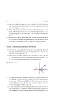
21. The two charges are located along a line as shown in the
2Q
diagram.
Q
(a) If the signs of the charges are opposite then the point on
the line where E = 0 will lie to the left of Q. In that region
ℓ
the electric fields from the two charges will point in
opposite directions, and the point will be closer to the
smaller charge.
(b) If the two charges have the same sign, then the point on the line where E = 0 will lie between
the two charges, closer to the smaller charge. In this region, the electric fields from the two
charges will point in opposite directions.
22. The electric field at point P would point in the negative x-direction. The magnitude of the field
would be the same as that calculated for a positive distribution of charge on the ring:

E

1

Qx

4 o  x 2  a 2 3/ 2

23. The velocity of the test charge will depend on its initial velocity. The field line gives the direction of
the change in velocity, not the direction of the velocity. The acceleration of the test charge will be
along the electric field line.
24. The value measured will be slightly less than the electric field value at that point before the test
charge was introduced. The test charge will repel charges on the surface of the conductor and these
charges will move along the surface to increase their distances from the test charge. Since they will
then be at greater distances from the point being tested, they will contribute a smaller amount to the
field.

© 2009 Pearson Education, Inc., Upper Saddle River, NJ. All rights reserved. This material is protected under all copyright laws as they
currently exist. No portion of this material may be reproduced, in any form or by any means, without permission in writing from the publisher.

3


Physics for Scientists & Engineers with Modern Physics, 4th Edition

Instructor Solutions Manual

25. The motion of the electron in Example 21-16 is projectile motion. In the case of the gravitational
force, the acceleration of the projectile is in the same direction as the field and has a value of g; in
the case of an electron in an electric field, the direction of the acceleration of the electron and the
field direction are opposite, and the value of the acceleration varies.
26. Initially, the dipole will spin clockwise. It will “overshoot” the equilibrium position (parallel to the
field lines), come momentarily to rest and then spin counterclockwise. The dipole will continue to
oscillate back and forth if no damping forces are present. If there are damping forces, the amplitude
will decrease with each oscillation until the dipole comes to rest aligned with the field.
27. If an electric dipole is placed in a nonuniform electric field, the charges of the dipole will experience
forces of different magnitudes whose directions also may not be exactly opposite. The addition of
these forces will leave a net force on the dipole.

Solutions to Problems
1.

Use Coulomb’s law to calculate the magnitude of the force.
1.602 1019 C 26 1.602 1019 C
Q1Q2
9
2
2
F  k 2  8.988 10 N  m C
 2.7 103 N
2

12
r
1.5 10 m



2.











Use Coulomb’s law to calculate the magnitude of the force.

Q1Q2
r2

1.602  10 C
C 
 4.0  10 m
19



 8.988  10 N  m
9

2

2

15

2

2

 14 N

The charge on the plastic comb is negative, so the comb has gained electrons.

 3.0  10 C  1.6021e 10


6

m
m
6.





Use Coulomb’s law to calculate the magnitude of the force.
25  106 C 2.5  103 C
Q1Q2
9
2
2
F  k 2  8.988  10 Nm C
 7200 N
r
 0.28m2

F k

5.







4.



Use the charge per electron to find the number of electrons.
 1 electron   2.37  1014 electrons
38.0  106 C 

19
 1.602  10 C 



3.







 9.109  1031 kg 
19

C 

1e

  4.9  1016  4.9  1014%

0.035kg

Since the magnitude of the force is inversely proportional to the square of the separation distance,
1
F  2 , if the distance is multiplied by a factor of 1/8, the force will be multiplied by a factor of 64.
r





F  64F0  64 3.2 102 N  2.0 N

© 2009 Pearson Education, Inc., Upper Saddle River, NJ. All rights reserved. This material is protected under all copyright laws as they
currently exist. No portion of this material may be reproduced, in any form or by any means, without permission in writing from the publisher.

4


Chapter 21

Electric Charges and Electric Field

7.

Since the magnitude of the force is inversely proportional to the square of the separation distance,

1
F  2 , if the force is tripled, the distance has been reduced by a factor of 3 .
r
r
8.45 cm
r 0 
 4.88 cm
3
3

8.

Use the charge per electron and the mass per electron.
 1 electron   2.871  1014  2.9  1014 electrons
46  106 C 

19
 1.602  10 C 





 2.871  10 e   9.1091e10
14

kg 

16
  2.6  10 kg







9.

31



To find the number of electrons, convert the mass to moles, the moles to atoms, and then multiply by
the number of electrons in an atom to find the total electrons. Then convert to charge.
 1mole Al   6.022  1023 atoms   79 electrons   1.602  1019 C 
15kg Au  15kg Au  

  1molecule  

1 mole
electron
 0.197 kg  



 5.8  108 C

The net charge of the bar is 0C , since there are equal numbers of protons and electrons.
10. Take the ratio of the electric force divided by the gravitational force.
QQ

2
9
2
2
19
k 12 2
8.988

10
N

m
C
1.602

10
C
FE
kQ
Q
1 2
r



 2.3 1039
11
31
27
2

2
mm
FG
Gm1m2
6.67 10 N  m kg 9.1110 kg 1.67 10 kg
G 12 2
r
The electric force is about 2.3 1039 times stronger than the gravitational force for the given scenario.















11. (a) Let one of the charges be q , and then the other charge is QT  q. The force between the
charges is FE  k

q  QT  q 

d 2 FE
dq

2



2k
r2



k





qQT  q2 . To find the maximum and minimum force, set the
r
r2
first derivative equal to 0. Use the second derivative test as well.
k
dFE k
2
  QT  2q   0  q  12 QT
FE  2  qQT  q  ;
r
dq r 2
2

 0  q  12 QT gives  FE  max

So q1  q2  12 QT gives the maximum force.
(b) If one of the charges has all of the charge, and the other has no charge, then the force between
them will be 0, which is the minimum possible force. So q1  0, q2  QT gives the minimum
force.

© 2009 Pearson Education, Inc., Upper Saddle River, NJ. All rights reserved. This material is protected under all copyright laws as they
currently exist. No portion of this material may be reproduced, in any form or by any means, without permission in writing from the publisher.

5


Physics for Scientists & Engineers with Modern Physics, 4th Edition

Instructor Solutions Manual

12. Let the right be the positive direction on the line of charges. Use the fact that like charges repel and
unlike charges attract to determine the direction of the forces. In the following expressions,
k  8.988  109 N  m2 C2 .

 75C 48C ˆ  75C85C ˆ
F75  k
ik
i  147.2 N ˆi  150 N ˆi
 0.35m2
 0.70 m2

 75C 48C ˆ  48C85C ˆ
F48  k
ik

i  563.5 N ˆi  560 N ˆi
 0.35m2
 0.35m2

85C 75C ˆ 85C 48C ˆ
F85  k
ik
i  416.3 N ˆi  420 N ˆi
2
2
0.70
m
0.35m




13. The forces on each charge lie along a line connecting the charges. Let the
variable d represent the length of a side of the triangle. Since the triangle
is equilateral, each angle is 60o. First calculate the magnitude of each
individual force.

F12  k

Q1Q2
d2



 8.988  10 N  m C

9

2

2



 7.0  10 C8.0  10 C
6


F13

1.20 m 


F23

2

Q1Q3
d2



 8.988  109 N  m2 C2



Q2

d
Q3

d


F21

 0.3495 N
F13  k

Q1

d

6


F12


F32

F31

 7.0  10 C 6.0  10 C
6

6

1.20 m2

 0.2622 N

F23  k

Q2Q3
d2



 8.988 10 N  m C
9

2

2



8.0 10 C 6.0 10 C  0.2996 N  F
6

6

1.20 m 2

32

Now calculate the net force on each charge and the direction of that net force, using components.
F1 x  F12 x  F13 x    0.3495 N  cos 60o   0.2622 N  cos 60o  4.365  102 N
F1 y  F12 y  F13 y    0.3495 N  sin 60o   0.2622 N  sin 60o  5.297  101 N
F1  F12x  F12y  0.53N

1  tan 1

F1 y

 tan 1

F1x

5.297  101 N

 265

4.365  102 N

F2 x  F21x  F23 x   0.3495 N  cos 60o   0.2996 N   1.249  101 N
F2 y  F21 y  F23 y   0.3495 N  sin 60o  0  3.027  101 N
F2  F22x  F22y  0.33 N

2  tan 1

F2 y
F2 x

 tan 1

3.027  101 N
1.249  101 N

 112

F3 x  F31 x  F32 x    0.2622 N  cos 60o   0.2996 N   1.685  101 N
F3 y  F31 y  F32 y   0.2622 N  sin 60o  0  2.271  101 N
F3  F32x  F32y  0.26 N

3  tan 1

F3 y
F3 x

 tan 1

2.271  101 N
1.685  101 N

 53

© 2009 Pearson Education, Inc., Upper Saddle River, NJ. All rights reserved. This material is protected under all copyright laws as they
currently exist. No portion of this material may be reproduced, in any form or by any means, without permission in writing from the publisher.

6


Chapter 21

Electric Charges and Electric Field

14. (a) If the force is repulsive, both charges must be positive since the total charge is positive. Call the
total charge Q.
kQ  Q  Q 
kQ Q
Fd 2
Q1  Q2  Q
F  12 2  1 2 1
 Q12  QQ1 
0
d
d
k
Q  Q2  4
Q1 

Fd 2
k

Q  Q2  4


2


   90.0  106 C  


Fd 2

k

2

 90.0  10 C 
6

1
2

2

4



8.988  109 N  m2 C2  

12.0N 1.16 m 2

 60.1  106 C , 29.9  10 6 C
(b) If the force is attractive, then the charges are of opposite sign. The value used for F must then
be negative. Other than that, the solution method is the same as for part (a).
kQ  Q  Q 
kQ Q
Fd 2
 Q12  QQ1 
0
Q1  Q2  Q
F  12 2  1 2 1

d
d
k

Q  Q2  4
Q1 

Fd 2
k



2





Q  Q2  4





k

2



 12  90.0  106 C 

Fd 2

90.0  106 C



2

4

 12.0N 1.16 m  2 

8.988  10

9





N  m 2 C2 


 106.8  106 C ,  16.8  106 C
15. Determine the force on the upper right charge, and then use the
symmetry of the configuration to determine the force on the other three
charges. The force at the upper right corner of the square is the vector
sum of the forces due to the other three charges. Let the variable d

represent the 0.100 m length of a side of the square, and let the variable
Q represent the 4.15 mC charge at each corner.

F41  k
F42  k
F43  k

Q2
d2
Q2
2d 2
Q2

 F41x  k

Q2
d2

 F42 x  k

, F41 y  0

Q2
2d 2

 F43 x  0 , F43 y  k

Q1

2Q 2

4d 2

, F42 y  k

Q4


F41

d

Q2

cos45o  k


F42


F43

Q3

2Q 2
4d 2

Q2

d2
d2

Add the x and y components together to find the total force, noting that F4 x  F4 y .

F4 x  F41x  F42 x  F43 x  k
F4  F42x  F42y  k

Q2 
2

Q2
d2

1 

d 

k

2Q 2
4d 2

0  k

2

Q2 

4 

2

 2 k

Q2 

2

1

  F4 y
d2 
4 

1
 2 
d 
2

© 2009 Pearson Education, Inc., Upper Saddle River, NJ. All rights reserved. This material is protected under all copyright laws as they
currently exist. No portion of this material may be reproduced, in any form or by any means, without permission in writing from the publisher.

7


Physics for Scientists & Engineers with Modern Physics, 4th Edition



 8.988  10 N  m C
9

  tan 1

2

2



 4.15  10 C
3

 0.100 m 

2

2

Instructor Solutions Manual

 2  1   2.96  107 N


2


F4 y

 45o above the x-direction.
F4 x
For each charge, the net force will be the magnitude determined above, and will lie along the line

from the center of the square out towards the charge.
16. Determine the force on the upper right charge, and then use the symmetry of the configuration to
determine the force on the other charges.
The force at the upper right corner of the square is the vector sum of the
forces due to the other three charges. Let the variable d represent the
0.100 m length of a side of the square, and let the variable Q represent
the 4.15 mC charge at each corner.
Q2
Q2
F41  k 2  F41x  k 2 , F41 y  0
d
d

F42  k
F43  k

Q2

 F42 x  k

2d 2
Q2

Q2
2d 2

2Q 2

cos45  k
o

 F43 x  0 , F43 y  k

4d 2

, F42 y  k


F41

Q1

Q4

F43

d

Q2

2Q2


F42

Q3

4d 2

Q2

d2
d2
Add the x and y components together to find the total force, noting that F4 x  F4 y .

Q2

F4 x  F41x  F42 x  F43 x  k
F4  F42x  F42y  k

d2

k

Q2
d

 0.64645
2

2Q 2
4d 2
2 k

0  k
Q2
d2



 8.988  10 N  m

  tan 1

F4 y

2

2

Q2

d2 

4 

d2

 1 

  0.64645k

 F4 y

 0.9142 

 4.15  10 C  0.9142  1.42  10 N
C 
2

3

9

Q2 

2

7

 0.100 m 

2

 225o from the x-direction, or exactly towards the center of the square.

F4 x
For each charge, there are two forces that point towards the adjacent corners, and one force that
points away from the center of the square. Thus for each charge, the net force will be the magnitude
of 1.42  107 N and will lie along the line from the charge inwards towards the center of the square.
17. The spheres can be treated as point charges since they are spherical, and so Coulomb’s law may be
used to relate the amount of charge to the force of attraction. Each sphere will have a magnitude Q
of charge, since that amount was removed from one sphere and added to the other, being initially
uncharged.

F k

Q1Q2
r2

k

Q2
r2

 Qr

F
k

  0.12 m 

1.7 102 N
8.988 109 N  m2 C2

 1 electron 
12
  1.0 10 electrons
19
 1.602 10 C 

 1.650 107 C 

© 2009 Pearson Education, Inc., Upper Saddle River, NJ. All rights reserved. This material is protected under all copyright laws as they
currently exist. No portion of this material may be reproduced, in any form or by any means, without permission in writing from the publisher.

8


Chapter 21

Electric Charges and Electric Field

18. The negative charges will repel each other, and so the third charge
Q
Q0
4Q0
must put an opposite force on each of the original charges.
Consideration of the various possible configurations leads to the
x
l–x
conclusion that the third charge must be positive and must be between
the other two charges. See the diagram for the definition of variables.
l
For each negative charge, equate the magnitudes of the two forces on the charge. Also note that
0  x  l.

left: k
k

Q0Q

k

Q0Q

x
x

2

2

Q0Q

k

x2
k
k

4Q02
l2

4Q0Q

 l  x
4Q02
l

2

4Q0Q

right: k

 l  x 2

k

4Q02



l2

 x  13 l

2

 Q  4Q0

x2
l

 Q0

2

Thus the charge should be of magnitude

4
9

4

 3

2

 94 Q0

Q0 , and a distance

1
3

l from  Q0 towards  4Q0 .

19. (a) The charge will experience a force that is always pointing
q
Q
Q
towards the origin. In the diagram, there is a greater force of
dx
dx
Qq
Qq
to the left, and a lesser force of
to
2
2
4 0  d  x 
4 0  d  x 
the right. So the net force is towards the origin. The same would be true if the mass were to the
left of the origin. Calculate the net force.
Qq
Qq
Qq
 d  x  2   d  x  2 

Fnet 


2
2
2
2 

4 0  d  x  4 0  d  x  4 0  d  x   d  x 


4Qqd

4 0  d  x   d  x 
2

2

x

Qqd

 0  d  x   d  x 
2

2

x

We assume that x  d .

Qqd
Qq
Fnet 
x
x
2
2
 0d 3
 0  d  x   d  x 
This has the form of a simple harmonic oscillator, where the “spring constant” is kelastic 

Qq

 0d 3

.

The spring constant can be used to find the period. See Eq. 14-7b.
T  2

m
kelastic

m
Qq

 2

 0d

 2

m 0d 3
Qq

3

(b) Sodium has an atomic mass of 23.
T  2

m 0d 3
Qq

 2

 29 1.66  1027 kg   8.85  1012 C2

1.60  10

19

C



N m2

 3  10

10

m



3

2

 1012 ps 
  0.24 ps  0.2 ps
 1s 

 2.4  1013 s 

© 2009 Pearson Education, Inc., Upper Saddle River, NJ. All rights reserved. This material is protected under all copyright laws as they
currently exist. No portion of this material may be reproduced, in any form or by any means, without permission in writing from the publisher.

9


Physics for Scientists & Engineers with Modern Physics, 4th Edition

Instructor Solutions Manual

20. If all of the angles to the vertical (in both cases) are assumed to


be small, then the spheres only have horizontal displacement,
FT1

FT2
1
2
and so the electric force of repulsion is always horizontal.
Likewise, the small angle condition leads to tan   sin   


for all small angles. See the free-body diagram for each sphere,

FE1 m g
F
E2
m2g
1
showing the three forces of gravity, tension, and the
electrostatic force. Take to the right to be the positive
horizontal direction, and up to be the positive vertical direction. Since the spheres are in equilibrium,
the net force in each direction is zero.
(a)  F1x  FT1 sin 1  FE1  0  FE1  FT1 sin 1

F

1y

 FT1 cos 1  m1 g  FT1 

m1 g
cos 1

 FE1 

m1 g
cos 1

sin 1  m1 g tan 1  m1 g1

A completely parallel analysis would give FE2  m2 g 2 . Since the electric forces are a
Newton’s third law pair, they can be set equal to each other in magnitude.
FE1  FE2  m1 g1  m2 g 2  1  2  m2 m1  1
(b) The same analysis can be done for this case.
FE1  FE2  m1 g1  m2 g 2  1  2  m1 m1  2
(c) The horizontal distance from one sphere to the other is
s by the small angle approximation. See the diagram. Use the
relationship derived above that FE  mg to solve for the distance.

Case 1:

d  l 1  2   2l1  1 
m1 g1  FE1 

Case 2:

kQ  2Q 
d2

d  l 1  2  
m1 g1  FE1 

3
2

kQ  2Q 
d2

d
2l
1/ 3

 4lkQ 2 
 mg
 d 

2l
 mg 
d

l1  1 
 mg

2d
3l

l 1 2 l

l sin  1

l sin  2

2d
3l

1/ 3

 3lkQ 2 

 mg 

 d 

21. Use Eq. 21–3 to calculate the force. Take east to be the positive x direction.

 F


E
 F  qE  1.602  1019 C 1920 N C ˆi  3.08  1016 N ˆi  3.08  1016 N west
q







22. Use Eq. 21–3 to calculate the electric field. Take north to be the positive y direction.

 F 2.18  1014 N ˆj
E 
 1.36  105 N C ˆj  1.36  105 N C south
19
q

1.602  10 C
23. Use Eq. 21–4a to calculate the electric field due to a point charge.
Q
33.0  106 C
E  k 2  8.988  109 N  m2 C2
 1.10  107 N C up
2
r
 0.164 m
Note that the electric field points away from the positive charge.





© 2009 Pearson Education, Inc., Upper Saddle River, NJ. All rights reserved. This material is protected under all copyright laws as they
currently exist. No portion of this material may be reproduced, in any form or by any means, without permission in writing from the publisher.

10


Chapter 21

Electric Charges and Electric Field

24. Use Eq. 21–3 to calculate the electric field.

 F 8.4 N down
E 
 9.5 105 N C up

6
q 8.8 10 C
25. Use the definition of the electric field, Eq. 21-3.

 F
7.22  104 N ˆj
 172 N C ˆj
E 
q
4.20  106 C





26. Use the definition of the electric field, Eq. 21-3.

 F
3.0ˆi  3.9ˆj  103 N
 2400 ˆi  3100 ˆj N C
E 
q
1.25  106 C









27. Assuming the electric force is the only force on the electron, then Newton’s second law may be used
to find the acceleration.


1.602  1019 C
q

Fnet  ma  qE  a  E 
 576 N C  1.01  1014 m s2
31
m
9.109  10 kg







Since the charge is negative, the direction of the acceleration is opposite to the field .


E1

28. The electric field due to the negative charge will point
Q1  0
toward the negative charge, and the electric field due to the
positive charge will point away from the positive charge.

Thus both fields point in the same direction, towards the
l 2
negative charge, and so can be added.
Q
Q
Q1
Q2
4k
E  E1  E2  k 21  k 22  k
k
 2  Q1  Q2 
2
2
r1
r2
 l / 2
 l / 2 l





4 8.988  109 N  m2 C2

 0.080 m

2



8.0  10

6

Q2  0


E2



C  5.8  106 C  7.8  107 N C

The direction is towards the negative charge .
29.

30. Assuming the electric force is the only force on the electron, then Newton’s second law may be used
to find the electric field strength.
1.673  1027 kg 1.8  106 9.80 m s2
ma
Fnet  ma  qE  E 

 0.18 N C
q
1.602  1019 C












© 2009 Pearson Education, Inc., Upper Saddle River, NJ. All rights reserved. This material is protected under all copyright laws as they
currently exist. No portion of this material may be reproduced, in any form or by any means, without permission in writing from the publisher.

11


Physics for Scientists & Engineers with Modern Physics, 4th Edition

Instructor Solutions Manual

31. The field at the point in question is the vector sum of the two fields shown in Figure 21-56. Use the
results of Example 21-11 to find the field of the long line of charge.

1 ˆ 
1 Q
Ethread 
j ; EQ 
cos ˆi  sin  ˆj 
2 0 y
4 0 d 2





 
  1 

1 Q
1 Q
E  

cos   ˆi  
sin   ˆj
2
2
 4 0 d
  2 0 y 4 0 d


d 2   0.070 m    0.120 m   0.0193m2 ; y  0.070 m ;   tan 1
2

Ex  
Ey 

Q

1

4 0 d
1 

2 0 y



cos    8.988  109 N  m2 C2

2



2

Q

1

4 0 d

2

sin  



 0.0193m
2.0C

2

12.0cm

7.0cm

 59.7

cos59.7  4.699  1011 N C

1  2 Q

 2 sin  

4 0  y d


 2  2.5C m 

 2.0C
sin 59.7  1.622  1011 N C
 8.988  109 N  m2 C2 

2
 0.070cm 0.0193m







E  4.7  1011 N C ˆi  1.6  1011 N C ˆj



 



 4.699  10 N C    1.622  10
 1.622  10 N C  199
 4.699  10 N C

E  E x2  E y2 

2

11

11

N C



2

 5.0  1011 N C

11

 E  tan

1

11

32. The field due to the negative charge will point towards
the negative charge, and the field due to the positive charge
will point towards the negative charge. Thus the
magnitudes of the two fields can be added together to find
the charges.

Enet  2 EQ  2k

Q

 l / 2

2



8kQ
l

2

 Q

El2
8k




EQ

Q

 586 N C 0.160 m2



8 8.988  10 N  m C
2

33. The field at the upper right corner of the square is the vector sum of
the fields due to the other three charges. Let the variable l represent
the 1.0 m length of a side of the square, and let the variable Q represent
the charge at each of the three occupied corners.
Q
Q
E1  k 2  E1 x  k 2 , E1 y  0
l
l

E2  k
E3  k

Q
2l
Q

2

2

 E2 x  k

Q
2l

2

cos45o  k

 E3 x  0 , E1 y  k

2Q
4l

2


E Q

l 2

9

, E2 y  k

2Q

4l 2

Q

2



 2.09  1010 C

E3

Q1


E2

E1

l

Q2

Q3

Q

l
l2
Add the x and y components together to find the total electric field, noting that Ex  Ey .

© 2009 Pearson Education, Inc., Upper Saddle River, NJ. All rights reserved. This material is protected under all copyright laws as they
currently exist. No portion of this material may be reproduced, in any form or by any means, without permission in writing from the publisher.

12


Electric Charges and Electric Field

Chapter 21

E x  E1 x  E2 x  E3 x  k

E  Ex2  E y2  k

Q
l

2

4l

2

0k

Q

2
1 

  Ey
l 
4 
2

2
Q
1
1


 2 k 2 2 
2
4 
2
l 
l 



Ey

2Q

Q

 8.988  109 N  m2 C2

  tan 1

k



 2.25  10 C 
6

1.22 m


4
 2    2.60  10 N C
2


2

1

 45.0 from the x-direction.

Ex

34. The field at the center due to the two 27.0C negative charges
on opposite corners (lower right and upper left in the diagram)
will cancel each other, and so only the other two charges need to
be considered. The field due to each of the other charges will
point directly toward the charge. Accordingly, the two fields are
in opposite directions and can be combined algebraically.
Q

Q
Q Q
E  E1  E2  k 2 1  k 2 2  k 1 2 2
l 2
l 2
l 2



 8.988  109 N  m2 C2




E1

l

Q1  38.6  C

38.6  27.0  10 C
6

 0.525m 2

Q2  27.0  C

Q2



E2
Q2

2

 7.57  106 N C, towards the  38.6C charge
35. Choose the rightward direction to be positive. Then the field due to +Q will be positive, and the
field due to –Q will be negative.

Ek

Q

 x  a

2

k

Q

 x  a

2

 1

1
4kQxa




2
2
  x  a  x  a 
2
2 2

 x a 

 kQ 

The negative sign means the field points to the left .
36. For the net field to be zero at point P, the magnitudes of the fields created by Q1 and Q2 must be
equal. Also, the distance x will be taken as positive to the left of Q1 . That is the only region where
the total field due to the two charges can be zero. Let the variable l represent the 12 cm distance,
and note that Q1  12 Q2 .


Q
Q2

E1  E2  k 21  k
x
 x  l 2

xl



Q1
Q2 

Q1



 12 cm 



25C
45C  25C



 35cm

© 2009 Pearson Education, Inc., Upper Saddle River, NJ. All rights reserved. This material is protected under all copyright laws as they
currently exist. No portion of this material may be reproduced, in any form or by any means, without permission in writing from the publisher.

13


Physics for Scientists & Engineers with Modern Physics, 4th Edition

Instructor Solutions Manual

37. Make use of Example 21-11. From that, we see that the electric field due to the line charge along the


1 ˆ
y axis is E1 
i. In particular, the field due to that line of charge has no y dependence. In a
2 0 x

1 ˆ
similar fashion, the electric field due to the line charge along the x axis is E2 
j. Then the
2 0 y

total field at  x, y  is the vector sum of the two fields.

  
1 ˆ
1 ˆ
  1 ˆ 1 ˆ
E  E1  E2 
i
j
 i  y j
2 0 x
2 0 y
2 0  x


E


2 0

1
x

2



1
y

2



1 
E
x
2 0 y
 tan 1
;   tan 1 y  tan 1
1

Ex
y
2 0 x


x2  y2
2 0 xy

38. (a) The field due to the charge at A will point straight downward, and
the field due to the charge at B will point along the line from A to
the origin, 30o below the negative x axis.
Q
Q
EA  k 2  EAx  0 , EAx  k 2
l
l
EB  k

Q
l

2

l
Q

EBy  k
E x  EAx  EBx  k
E  Ex2  E y2 

  tan

Q

 EBx  k

Ey
1

Ex

l2

4l



4

k
k

2l
Q

2

9k 2Q 2
4l



4

Q
l

Q

l


EB

,

B
l


EA

2l 2

E y  EAy  EBy  k

2

3k 2Q 2

 tan 1

sin 30o  k

3Q
2l

3Q

cos 30o  k
2

A

12k 2Q 2
4l

4

3Q
2l 2
3kQ



l2

3Q

2l 2  tan 1 3  tan 1 3  240o
3Q
 3

2l 2

(b) Now reverse the direction of EA
EA  k
EB  k

Q
l

2

Q
l

2

 EAx  0 , EAx  k
 EBx  k

E x  EAx  EBx  k
E  Ex2  E y2 

Q
l

2

4l

4

3Q
2l

2

, EBy  k

E y  EAy  EBy  k

2

3k 2Q 2

l2

cos 30o  k

3Q
2l

Q



k 2Q 2
4l

4



4k 2Q 2
4l

4



Q
l

2

sin 30o  k

Q
2l2

Q
2l 2

kQ
l2

© 2009 Pearson Education, Inc., Upper Saddle River, NJ. All rights reserved. This material is protected under all copyright laws as they
currently exist. No portion of this material may be reproduced, in any form or by any means, without permission in writing from the publisher.

14


Electric Charges and Electric Field

Chapter 21

  tan

Ey
1
Ex

Q

k

 tan 1

2l 2  tan 1 1  330o
3Q
 3

k

2l 2

39. Near the plate, the lines should come from it almost vertically,
because it is almost like an infinite line of charge when the
observation point is close. When the observation point is far
away, it will look like a point charge.

+

+

+

40. Consider Example 21-9. We use the result from this example, but
shift the center of the ring to be at x  12 l for the ring on the right,

Q  x  12 l 

1

4 0  x  1 l  2  R 2 
2



/ 2



+

y

and at x   12 l for the ring on the left. The fact that the original
expression has a factor of x results in the interpretation that the sign
of the field expression will give the direction of the field. No special
consideration needs to be given to the location of the point at which
the field is to be calculated.
 

E  Eright  Eleft



+

R

R
1
2

l

O

1
2

x

l

Q  x  12 l 
ˆi  1
ˆi
/ 2
4 0  x  1 l  2  R 2 
2









Q 
 x  12 l 
 x  12 l 

 ˆi


/ 2
/ 2 
2
2
4 0   x  1 l   R 2 
 x  12 l   R 2  
2











41. Both charges must be of the same sign so that the electric fields created by the two charges oppose
each other, and so can add to zero. The magnitudes of the two electric fields must be equal.

E1  E2  k

Q1

 l 3

2

k

Q2

 2l 3

 9Q1 

2

9Q2
4



Q1
Q2



1
4


42. In each case, find the vector sum of the field caused by the charge on the left Eleft and the field



Eright
caused by the charge on the right Eright
Eleft



 



Point A: From the symmetry of the geometry, in
calculating the electric field at point A only the vertical
components of the fields need to be considered. The
horizontal components will cancel each other.
5.0
  tan 1
 26.6
10.0
d

 5.0cm2  10.0cm 2

A
d
Q



d



Q

 0.1118 m

© 2009 Pearson Education, Inc., Upper Saddle River, NJ. All rights reserved. This material is protected under all copyright laws as they
currently exist. No portion of this material may be reproduced, in any form or by any means, without permission in writing from the publisher.

15


Physics for Scientists & Engineers with Modern Physics, 4th Edition

EA  2

kQ
d



sin  2 8.988  109 N  m2 C2

2

Instructor Solutions Manual

6

 10 C
sin 26.6  3.7  10
 5.7
0.1118 m

6





2

Point B: Now the point is not symmetrically placed, and
so horizontal and vertical components of each individual
field need to be calculated to find the resultant electric
field.
5.0
5.0
left  tan 1
 45
right  tan 1

 18.4
5.0
15.0
d left 

 5.0cm

d right 

 5.0cm2  15.0cm 2

2

N C


Eright

 right

 left

Q

  5.0cm   0.0707 m


Eleft

d right

dleft

2

A  90

Q

 0.1581m



Q
Q
E x   Eleft  x   Eright  x  k 2 cosleft  k 2 cos  right
d left
d right



 8.988  109 N  m2 C2



 5.7  10 C 
6

cos45

  0.0707 m 

2



2



cos18.4 

6
  5.30  10 N C
 0.1581m  
2



Q
Q
E y   Eleft  y   Eright  y  k 2 sinleft  k 2 sin  right
d left
d right



 8.988  109 N  m2 C2



 5.7  10 C 
6

sin45

  0.0707 m 

 B  tan 1

EB  Ex2  E y2  9.5  106 N C

sin18.4 

6
  7.89  10 N C
 0.1581m  
2

Ey

 56
Ex
The results are consistent with Figure 21-34b. In the figure, the field at Point A points straight up,
matching the calculations. The field at Point B should be to the right and vertical, matching the
calculations. Finally, the field lines are closer together at Point B than at Point A, indicating that the
field is stronger there, matching the calculations.
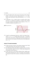
y

43. (a) See the diagram. From the symmetry of the charges, we see that

the net electric field points along the y axis.

Q
Qy
ˆj
E2
sin  ˆj 
2
2
2
2 3/ 2
4 0 l  y
2 0 l  y







dE
dy



Q



2 0 l 2  y



l y




r

Q

+


¬

E

2

y
¬

+

Q x



1
2

E1



(b) To find the position where the magnitude is a maximum, set the
first derivative with respect to y equal to 0, and solve for the y
value.
Qy

E
3/ 2
2 0 l 2  y 2



E

2 3/ 2





2 3/ 2

   23 

3y2



l y
2



2 5/ 2

Qy



2 0 l 2  y 2



5/ 2

2 y  0

 y 2  12 l 2  y   l



2

© 2009 Pearson Education, Inc., Upper Saddle River, NJ. All rights reserved. This material is protected under all copyright laws as they

currently exist. No portion of this material may be reproduced, in any form or by any means, without permission in writing from the publisher.

16


Electric Charges and Electric Field

Chapter 21

This has to be a maximum, because the magnitude is positive, the field is 0 midway between the
charges, and E  0 as y  .

44. From Example 21-9, the electric field along the x-axis is E 

1

Qx



4 0 x  a 2
2



3
2

. To find the position

where the magnitude is a maximum, we differentiate and set the first derivative equal to zero.
dE



dx



Q

x

2

 a2



4 0
Q

3
2



 x 23 x 2  a 2

x

2

a



2 3



1
2

2x



Q



4 0 x  a
2

2



5

2

 x 2  a 2   3x 2 

a



4 0 x 2  a 2



5
2

a 2  2 x 2   0  xM  
2

Note that E  0 at x  0 and x   , and that E  0 for 0  x   . Thus the value of the magnitude
of E at x  xM must be a maximum. We could also show that the value is a maximum by using the
second derivative test.
45. Because the distance from the wire is much smaller than the length of the wire, we can approximate
the electric field by the field of an infinite wire, which is derived in Example 21-11.
 4.75  106 C 
2
6
1 
1 2 
Nm2   2.0 m  1.8  10 N C,


  8.988  109

E

2 0 x 4 0 x 
C2   2.4  102 m 
away from the wire
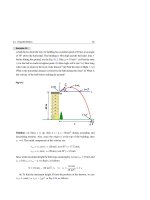
46. This is essentially Example 21-11 again, but with different limits of
integration. From the diagram here, we see that the maximum
l2
angle is given by sin  
. We evaluate the results at
2
x 2   l 2

y
dq

dy
y

E


 sin  
4 0 x
sin  

l 2
x  l 2 

2

2

2


l

l
 

1/ 2
2
2
2
 4 x x   l 2 
2 0 x  4 x  l 2 
0


47. If we consider just one wire, then from the answer to problem 46, we
would have the following. Note that the distance from the wire to the
point in question is x  z 2   l 2 .
2


2 0

z   l 2

2

x


dE

l 2
x  l 2 


 
l2
l 2



2
2
2
2
4 0 x  x   l 2  
x   l 2



Ewire 

x

l

2

P



that angle.
sin  

r

2



wire

wire

l

4  z   l 2    l
2

Eleft

Eright 

2

2





1/ 2

But the total field is not simply four times the above expression,
because the fields due to the four wires are not parallel to each other.

z2   l 2

2

z
l 2

l 2

© 2009 Pearson Education, Inc., Upper Saddle River, NJ. All rights reserved. This material is protected under all copyright laws as they
currently exist. No portion of this material may be reproduced, in any form or by any means, without permission in writing from the publisher.

17


Physics for Scientists & Engineers with Modern Physics, 4th Edition

Instructor Solutions Manual

Consider a side view of the problem. The two dots represent two parallel wires, on opposite sides of
the square. Note that only the vertical component of the field due to each wire will actually
contribute to the total field. The horizontal components will cancel.
z
Ewire  4  Ewire  cos   4  Ewire 
2
z 2   l 2
Ewire



 4
 2 0




z

1/ 2
2
2
 z 2   l 22
z 2   l 2  4  z 2   l 2    l 2

l





8 lz

 0  4 z 2  l 2  4 z 2  2 l 2 

1/ 2

The direction is vertical, perpendicular to the loop.
48. From the diagram, we see that the x components of the two fields will cancel each other at the point
P. Thus the net electric field will be in the negative
Q
y-direction, and will be twice the y-component of
either electric field vector.
a
kQ
Enet  2 E sin   2 2
sin 
2
x

x a


E
a
2kQ
Q
E Q

 2
a
1/ 2
x  a2 x2  a2







2 kQa

x

2

 a2



3/ 2

Q

in the negative y direction

49. Select a differential element of the arc which makes an
angle of  with the x axis. The length of this element
is Rd , and the charge on that element is dq   Rd .

The magnitude of the field produced by that element is
1  Rd
dE 
. From the diagram, considering
4 0 R 2
pieces of the arc that are symmetric with respect to the x
axis, we see that the total field will only have an x
component. The vertical components of the field due to
symmetric portions of the arc will cancel each other.
So we have the following.
1  Rd
dE horizontal 
cos 
4 0 R 2
0

E horizontal 



 0

1
4 0

cos 

 Rd
R2


dEbottom


dEtop

Rd

R


x

0

0





2 sin  0
cos  d 
sin  0  sin   0  

4 0 R 
4 0 R
4 0 R
0

The field points in the negative x direction, so E  

2 sin  0 ˆ
i
4 0 R

© 2009 Pearson Education, Inc., Upper Saddle River, NJ. All rights reserved. This material is protected under all copyright laws as they
currently exist. No portion of this material may be reproduced, in any form or by any means, without permission in writing from the publisher.

18


Electric Charges and Electric Field

Chapter 21

50. (a) Select a differential element of the arc which makes an
angle of  with the x axis. The length of this element
dQ   Rd
is Rd , and the charge on that element is dq   Rd .
The magnitude of the field produced by that element is

1  Rd
From
the
diagram,
considering
dE 
.



4 0 R 2


dE
pieces of the arc that are symmetric with respect to the dE
x axis, we see that the total field will only have a y
component, because the magnitudes of the fields due
to those two pieces are the same. From the diagram
we see that the field will point down. The horizontal components of the field cancel.
1  Rd
0
dE vertical 
sin  
sin 2  d
2
4 0 R
4 0 R
 /2

E vertical 


 /2




 /2
2

2
 400 R sin  d  400 R  sin  d  400 R  12   14 sin 2  / 2
 / 2
 / 2
0

 12    0
4 0 R
8 0 R



 E   0 ˆj
8 0 R

(b) The force on the electron is given by Eq. 21-3. The acceleration is found from the force.


q0 ˆ

F  m a  qE  
j 
8 0 R








1.60  10 19 C 1.0  10 6 C m
q0 ˆ
e0 ˆ

ˆj
a
j
j
8m 0 R
8m 0 R
8 9.11  10 31 kg 8.85  10 12 C 2 N  m 2  0.010 m 





 2.5  1017 m s 2 ˆj

51. (a) If we follow the first steps of Example 21-11, and refer to Figure 21-29, then the differential
1
 dy
electric field due to the segment of wire is still dE 
. But now there is no
2
4 0  x  y 2 
symmetry, and so we calculate both components of the field.
1
 dy
1

 x dy
dE x  dE cos  
cos  
3/ 2
2
2
4 0  x  y 
4 0  x 2  y 2 
dE y   dE sin   

1



 dy

4 0 x  y
2

2



sin   

 y dy

1



4 0 x  y 2
2



3/ 2

The anti-derivatives needed are in Appendix B4.
l

Ex  
0



 x dy

1



4 0 x 2  y 2



3/ 2

x


4 0

l


0

l

dy

x

2

 y2



3/ 2


x 
y

 2 2

4 0  x x  y 2 
0

l
4 0 x x 2  l 2

© 2009 Pearson Education, Inc., Upper Saddle River, NJ. All rights reserved. This material is protected under all copyright laws as they
currently exist. No portion of this material may be reproduced, in any form or by any means, without permission in writing from the publisher.

19


Physics for Scientists & Engineers with Modern Physics, 4th Edition

l

Ey  
0



 y dy

1





4 0 x 2  y 2




4 0

3/ 2

l

Instructor Solutions Manual

l

y dy



x

0

2

 y2



3/ 2


 
1


 2

4 0  x  y 2 
0



 
1
1

 
x  x2  l2

2
2
2
2
4 0  x  l
x  4 0 x x  l



Note that E y  0, and so the electric field points to the right and down.
(b) The angle that the electric field makes with the x axis is given as follows.

x  x2  l2
2
2
E y 4 0 x x  l

x  x2  l2
x
x2
tan  


  1 2
l
l
l
l
Ex





4 0 x x 2  l 2

As l  , the expression becomes tan   1 , and so the field makes an angle of
45 below the x axis .

52. Please note: the first printing of the textbook gave the length of the charged wire as 6.00 m, but it
should have been 6.50 m. That error has been corrected in later printings, and the following solution
uses a length of 6.50 m.
(a) If we follow the first steps of Example 21-11, and refer to Figure 21-29, then the differential
1
 dy
electric field due to the segment of wire is still dE 
. But now there is no

2
4 0  x  y 2 
symmetry, and so we calculate both components of the field.
1
 dy
1
 x dy
dE x  dE cos  
cos  
3/ 2
2
2
2
4 0  x  y 
4 0  x  y 2 
dE y   dE cos   

1



 dy

4 0 x  y
2

2



sin   

 y dy

1



4 0 x  y 2
2



3/ 2

The anti-derivatives needed are in Appendix B4.
y max

Ex 



y min



 x dy

1



4 0 x 2  y 2



3/ 2

x

4 0

y
 
 2 max 2 
4 0 x  x  y max


y max



y min

y max

dy

x

y min
2
x 2  y min

2

 y2



3/ 2


x 
y

 2 2

4 0  x x  y 2 
y

min






N  m 2   3.15  10 C   6.50 m 


  8.99  109
C 2 
 0.250 m 

6






2.50 m

 0.250 m  2   2.50 m  2




 4.00 m 

2
2
 0.250 m    4.00 m  

 3.473  10 4 N C  3.5  10 4 N C

© 2009 Pearson Education, Inc., Upper Saddle River, NJ. All rights reserved. This material is protected under all copyright laws as they
currently exist. No portion of this material may be reproduced, in any form or by any means, without permission in writing from the publisher.

20

Electric Charges and Electric Field

Chapter 21

y max

Ey  



y min



 y dy

1



4 0 x 2  y 2



3/ 2

 
1


 2
2
4 0  x  y max




4 0
1
2
x 2  y min

y max



y min

y max

y dy

x

2

 y2



3/ 2


 
1

 2

4 0  x  y 2 
y

min






N  m 2   3.15  10 C 

  8.99  109
C 2   6.50 m 

6






1

 0.250 m  2   2.50 m  2



1

 0.250 m 2   4.00 m  2






 647 N C  650 N C

(b) We calculate the infinite line of charge result, and calculate the errors.
2
3.15  10 6 C 

2


9 Nm 
4
E

 2  8.99  10

  6.50 m  0.250 m   3.485  10 N m
2
2 0 x 4 0 x
C


Ex  E
E
Ey
E



 3.473  10 N C    3.485  10

 3.485  10 N m 
4

4

N m

4

 647 N C 

 3.485  10

4

N m





0.0034

 0.019

And so we see that E x is only about 0.3% away from the value obtained from the infinite line of
charge, and E y is only about 2% of the value obtained from the infinite line of charge. The
field of an infinite line of charge result would be a good approximation for the field due to this
wire segment.
53. Choose a differential element of the rod dx  a
distance x from the origin, as shown in the
diagram. The charge on that differential element is
Q
dq  dx . The variable x is treated as positive,
l
so that the field due to this differential element is dE 

y
O

dq
dx
1

x

dq

4 0  x  x

2



Q


dE
x
dx

4 0 l  x  x 

2

x

. Integrate

along the rod to find the total field.
l
l
l
Q
dx 

Q
dx 
Q 
1 
Q 1
1 





E   dE  




2
2

4 0 l  x  x 
4 0 l 0  x  x 
4 0 l  x  x  0 4 0 l  x x  l 
0


Q
4 0 x  x  l 

© 2009 Pearson Education, Inc., Upper Saddle River, NJ. All rights reserved. This material is protected under all copyright laws as they
currently exist. No portion of this material may be reproduced, in any form or by any means, without permission in writing from the publisher.

21


Physics for Scientists & Engineers with Modern Physics, 4th Edition

Instructor Solutions Manual

54. As suggested, we divide the plane into long narrow strips of width dy and length l. The charge on
the strip is the area of the strip times the charge per unit area: dq   ldy. The charge per unit length
dq
on the strip is  
  dy. From Example 21-11, the field due to that narrow strip is
l

 dy
dE 

. From Figure 21-68 in the textbook, we see that this field
2 0 y 2  z 2 2 0 y 2  z 2
does not point vertically. From the symmetry of the plate, there is another long narrow strip a
distance y on the other side of the origin, which would create the same magnitude electric field. The
horizontal components of those two fields would cancel each other, and so we only need calculate
the vertical component of the field. Then we integrate along the y direction to find the total field.
 dy
 zdy
dE 
; dE z  dE cos  
2
2

2 0  y 2  z 2 
2 0 y  z


E  Ez 

 zdy

 2  y





2

0

 z2



z

2 0



 y



dy
2



 z 1  1 y 

 tan

z  
2 0 z 



 z2


     

    
 tan 1     tan 1     

2 0
2 0  2  2   2 0

55. Take Figure 21-28 and add the angle  , measured from the –z axis,
as indicated in the diagram. Consider an infinitesimal length of the
ring ad. The charge on that infinitesimal length is dq    ad 



Q

a

 ad  

Q



y
ad 

a

d. The charge creates an infinitesimal electric

Q



r
x

d

P



dE

x


1 
1 dq
field, d E, with magnitude dE 

. From the z
2
4  x 2  a 2
4  r

symmetry of the figure, we see that the z component of d E will be cancelled by the z component
due to the piece of the ring that is on the opposite side of the y axis. The trigonometric relationships
give dEx  dE cos  and dE y   dE sin  sin  . The factor of sin  can be justified by noting that
dE y  0 when   0, and dE y   dE sin  when    2.

dEx  dE cos  
Ex 

d

Q

4   x  a
2

2



4   x  a
2



2 3/ 2

 d 
0

dE y  dE sin  sin   
Ey  



4   x  a
2



2 3/ 2



4  x 2  a 2

d

4   x  a
2





3/ 2

3/ 2

a
2

x2  a2

 sin d   4 
0



4   x 2  a 2
2

Qx

Q
2

d

Qx





Qa
2

x2  a2



Qx
2

x
2

sin   

Qa

2





x2  a2



3/ 2

Qa



4 2  x 2  a 2



3/ 2

sin d

  cos      cos0

© 2009 Pearson Education, Inc., Upper Saddle River, NJ. All rights reserved. This material is protected under all copyright laws as they
currently exist. No portion of this material may be reproduced, in any form or by any means, without permission in writing from the publisher.

22


Electric Charges and Electric Field

Chapter 21

 

2Qa



4 2  x 2  a 2



3/ 2

We can write the electric field in vector notation.

Qx
2Qa
Q
 xˆi  2a ˆj 
ˆi 
ˆj 
E


3/
2
3/
2
3/

2
 
4   x 2  a 2 
4 2   x 2  a 2 
4 0  x 2  a 2  
56. (a) Since the field is uniform, the electron will experience a constant force in the direction opposite
to its velocity, so the acceleration is constant and negative. Use constant acceleration
relationships with a final velocity of 0.
eE
F  ma  qE  eE  a  
; v 2  v02  2ax  0 
m








2

9.11  1031 kg 27.5  106 m s
v02
mv 2
x  

 0 
 0.189 m
eE  2eE 2 1.60  1019 C 11.4  103 N C

2a

2  
 m
(b) Find the elapsed time from constant acceleration relationships. Upon returning to the original
position, the final velocity will be the opposite of the initial velocity.
v  v0  at 
v02

t

v  v0
a















31
6

2v0
2mv0 2 9.11  10 kg 27.5  10 m s


 2.75  108 s
19
3
eE
1.60  10 C 11.4  10 N C
   eE


 m



57. (a) The acceleration is produced by the electric force.




Fnet  ma  qE  eE 








1.60  1019 C
e 

 2.0ˆi  8.0ˆj  104 N C  3.513  1015 ˆi  1.405  1016 ˆj m s2
a E
m
9.11  1031 kg 







 3.5  1015 m s2 ˆi  1.4  1016 m s2 ˆj

(b) The direction is found from the components of the velocity.
  
v  v  at   8.0  104 m s  ˆj   3.513  1015 ˆi  1.405  1016 ˆj m s2  1.0  109 s 
 3.513  106 ˆi  1.397  107 ˆj m s





tan 1

vy





 1.397  107 m s 
  256 or  104
6
 3.513  10 m s 

 tan 1 

vx
This is the direction relative to the x axis. The direction of motion relative to the initial
direction is measured from the y axis, and so is   166 counter-clockwise from the initial
direction.

58. (a) The electron will experience a force in the opposite direction to the electric field. Since the
electron is to be brought to rest, the electric field must be in the same direction as the initial
velocity of the electron, and so is to the right .
(b) Since the field is uniform, the electron will experience a constant force, and therefore have a
constant acceleration. Use constant acceleration relationships to find the field strength.
© 2009 Pearson Education, Inc., Upper Saddle River, NJ. All rights reserved. This material is protected under all copyright laws as they
currently exist. No portion of this material may be reproduced, in any form or by any means, without permission in writing from the publisher.

23


Physics for Scientists & Engineers with Modern Physics, 4th Edition

qE

F  qE  ma  a 
E



m v 2  v02
2qx

v 2  v02  2ax  v02  2

m

  mv

Instructor Solutions Manual

qE

x 

m

 9.109 10 kg  7.5 10 m s

2qx
2  1.602  10 C  0.040 m
31

2
0

5

2

19

 40 N C

 2 sig. fig.

59. The angle is determined by the velocity. The x component of the velocity is constant. The time to
pass through the plates can be found from the x motion. Then the y velocity can be found using
constant acceleration relationships.
x
eE x
x  v0t  t 
; vy  vy0  ayt  
v0
m v0
tan  

vy
vx




eE x
m v0



v0

1.60  10 C 5.0  10 N C  0.049 m  .4303

 9.11  10 kg 1.00  10 m s 
19

eEx
mv02

3

31

7

2



  tan 1  0.4303  23
60. Since the field is constant, the force on the electron is constant, and so the acceleration is constant.
Thus constant acceleration relationships can be used. The initial conditions are x0  0, y0  0,
v x 0  1.90 m s, and v y 0  0.


e 

e
e

 q 
F  ma  qE  a  E   E ; ax   Ex , a y   E y
m
m
m
m
eE
x  x0  v x 0t  12 a x t 2  v x 0t  x t 2
2m

1.60  10 C 2.00  10 N C  2.0s  3.2 m
 1.90 m s  2.0s  
2  9.11  10 kg 
eE
1.60  10 C 1.20  10 N C  2.0s
y  y v t a t  
t 
2m
2  9.11  10 kg 
19

11

2

31

19

0

y0

1
2

y

2

11

2

y

31

2

 4.2 m

61. (a) The field along the axis of the ring is given in Example 21-9, with the opposite sign because this
ring is negatively charged. The force on the charge is the field times the charge q. Note that if
x is positive, the force is to the left, and if x is negative, the force is to the right. Assume that
x  R.
q

1
 qQx
 qQx
 Q  x


F  qE 
3/
2
3/
2
4 0 x 2  R 2
4 0 x 2  R 2
4 0 R3









This has the form of a simple harmonic oscillator, where the “spring constant” is
Qq
kelastic 
.
4 0 R 3
(b) The spring constant can be used to find the period. See Eq. 14-7b.
T  2

m
kelastic

 2

m
Qq

 2

m4 0 R 3
Qq

 4

m 0 R3
Qq

4 0 R3

© 2009 Pearson Education, Inc., Upper Saddle River, NJ. All rights reserved. This material is protected under all copyright laws as they
currently exist. No portion of this material may be reproduced, in any form or by any means, without permission in writing from the publisher.

24


Electric Charges and Electric Field

Chapter 21

62. (a) The dipole moment is given by the product of the positive charge and the separation distance.







p  Ql  1.60  1019 C 0.68  109 m  1.088  1028 C m  1.1  1028 C m
(b) The torque on the dipole is given by Eq. 21-9a.

  pE sin   1.088  1028 Cm  2.2  104 N C   sin 90  2.4  1024 C m







(c)   pE sin   1.088  1028 C m 2.2  104 N C  sin 45  1.7  1024 N m
(d) The work done by an external force is the change in potential energy. Use Eq. 21-10.
W  U    pE cos final     pE cos initial   pE  cos initial  cos final 







 1.088  1028 C m 2.2  104 N C 1   1   4.8  1024 J
63. (a) The dipole moment is the effective charge of each atom times the separation distance.
p 3.4  1030 C m
p  Ql  Q  
 3.4  1020 C
1.0  1010 m
l
Q 3.4  1020 C
(b)

 0.21 No, the net charge on each atom is not an integer multiple of e. This
e 1.60  1019 C
is an indication that the H and Cl atoms are not ionized – they haven’t fully gained or lost an
electron. But rather, the electrons spend more time near the Cl atom than the H atom, giving the
molecule a net dipole moment. The electrons are not distributed symmetrically about the two
nuclei.
(c) The torque is given by Eq. 21-9a.

  pE sin    max  pE   3.4  1030 C m  2.5  104 N C   8.5  1026 N m

(d) The energy needed from an external force is the change in potential energy. Use Eq. 21-10.
W  U    pE cos final     pE cos initial   pE  cos initial  cos final 







 3.4  1030 C m 2.5  104 N C 1  cos 45  2.5  1026 J

64. (a) From the symmetry in the diagram, we see that the resultant field
will be in the y direction. The vertical components of the two
fields add together, while the horizontal components cancel.
Q
r
Enet  2 E sin   2
1/ 2
2
2
4 0 r  l
r2  l2





2Qr



4 0 r 2  l 2



3/ 2





2Qr

 

4 0 r 3

y

E





2Q
4 0 r 2

r


Q
+

¬

(b) Both charges are the same sign. A long distance away from the
charges, they will look like a single charge of magnitude 2Q, and so E  k



E

q
r

2

Q
+ x

¬


2Q
4 0 r 2

.

65. (a) There will be a torque on the dipole, in a direction to decrease  . That torque will give the
dipole an angular acceleration, in the opposite direction of  .

   pE sin   I   

d 2
dt

2



pE
I

sin 

© 2009 Pearson Education, Inc., Upper Saddle River, NJ. All rights reserved. This material is protected under all copyright laws as they
currently exist. No portion of this material may be reproduced, in any form or by any means, without permission in writing from the publisher.

25