Ebook mechanics of materials (7th edition) part 2

A more advanced theory is required for analysis and design of composite beams and beams with unsymmetric cross sections.


6
Stresses in Beams
(Advanced Topics)
CHAPTER OVERVIEW
In Chapter 6, we will consider a number of advanced topics related to
shear and bending of beams of arbitrary cross section. First, stresses and
strains in composite beams, that is beams fabricated of more than one
material, is discussed in Section 6.2. First, we locate the neutral axis
then find the flexure formula for a composite beam made up of two different materials. We then study the transformed-section method as an
alternative procedure for analyzing the bending stresses in a composite
beam in Section 6.3. Next, we study bending of doubly symmetric
beams acted on by inclined loads having a line of action through the
centroid of the cross section (Section 6.4). In this case, there are bending
moments (My, Mz) about each of the principal axes of the cross section,
and the neutral axis is no longer perpendicular to the longitudinal plane
containing the applied loads. The final normal stresses are obtained by
superposing the stresses obtained from the flexure formulas for each of
the separate axes of the cross section. Next, we investigate the general
case of unsymmetric beams in pure bending, removing the restriction of
at least one axis of symmetry in the cross section (Section 6.5). We
develop a general procedure for analyzing an unsymmetric beam subjected to any bending moment M resolved into components along the
principal centroidal axes of the cross section. Of course, symmetric
beams are special cases of unsymmetric beams, and therefore, the discussions also apply to symmetric beams. If the restriction of pure
bending is removed and transverse loads are allowed, we note that these
loads must act through the shear center of the cross section so that twisting of the beam about a longitudinal axis can be avoided (Sections 6.6
and 6.9). The distributions of shear stresses in the elements of the cross
sections of a number of beams of thin-walled open section (such as
channels, angles, and Z shapes) are calculated and then used to locate

the shear center for each particular cross-sectional shape (Sections 6.7,
6.8 and 6.9). As the final topic in the chapter, the bending of elastoplastic beams is described in which the normal stresses go beyond the linear
elastic range of behavior (Section 6.10).

455


456

CHAPTER 6

Stresses in Beams (Advanced Topics)

Chapter 6 is organized as follows:
6.1 Introduction

457

6.2 Composite Beams
6.3
6.4
6.5
6.6
6.7
6.8
6.9
*6.10

457
Transformed-Section Method 466

Doubly Symmetric Beams with Inclined Loads 472
Bending of Unsymmetric Beams 479
The Shear-Center Concept 487
Shear Stresses in Beams of Thin-Walled Open Cross Sections 489
Shear Stresses in Wide-Flange Beams 492
Shear Centers of Thin-Walled Open Sections 496
Elastoplastic Bending 504
Chapter Summary & Review 514
Problems 516
*
Advanced Topics


SECTION 6.2

Composite Beams

457

6.1 INTRODUCTION
In this chapter, we continue our study of the bending of beams by examining several specialized topics. These subjects are based upon the
fundamental topics discussed previously in Chapter 5—topics such as
curvature, normal stresses in beams (including the flexure formula), and
shear stresses in beams. However, we will no longer require that beams
be composed of one material only; and we will also remove the restriction that the beams have a plane of symmetry in which transverse loads
must be applied. Finally, we will extend the performance into the inelastic range of behavior for beams made of elastoplastic materials.
Later, in Chapters 9 and 10, we will discuss two additional subjects
of fundamental importance in beam design—deflections of beams and
statically indeterminate beams.

6.2 COMPOSITE BEAMS

(a)

(b)

Beams that are fabricated of more than one material are called composite beams. Examples are bimetallic beams (such as those used in
thermostats), plastic coated pipes, and wood beams with steel reinforcing plates (see Fig. 6-1).
Many other types of composite beams have been developed in
recent years, primarily to save material and reduce weight. For instance,
sandwich beams are widely used in the aviation and aerospace industries, where light weight plus high strength and rigidity are required.
Such familiar objects as skis, doors, wall panels, book shelves, and
cardboard boxes are also manufactured in sandwich style.
A typical sandwich beam (Fig. 6-2) consists of two thin faces of
relatively high-strength material (such as aluminum) separated by a
thick core of lightweight, low-strength material. Since the faces are at
the greatest distance from the neutral axis (where the bending stresses
are highest), they function somewhat like the flanges of an I-beam. The
core serves as a filler and provides support for the faces, stabilizing
them against wrinkling or buckling. Lightweight plastics and foams, as
well as honeycombs and corrugations, are often used for cores.

Strains and Stresses

(c)

(c)

FIG. 6-1 Examples of composite beams:
(a) bimetallic beam, (b) plastic-coated

steel pipe, and (c) wood beam reinforced with a steel plate

The strains in composite beams are determined from the same basic axiom
that we used for finding the strains in beams of one material, namely, cross
sections remain plane during bending. This axiom is valid for pure bending
regardless of the nature of the material (see Section 5.4). Therefore, the
longitudinal strains ex in a composite beam vary linearly from top to bottom of the beam, as expressed by Eq. (5-4), which is repeated here:
y
ex ϭ Ϫ ᎏᎏ ϭ Ϫky
r

(6-1)


458

CHAPTER 6

Stresses in Beams (Advanced Topics)

(a)

(b)

(c)

In this equation, y is the distance from the neutral axis, r is the radius of
curvature, and k is the curvature.
Beginning with the linear strain distribution represented by Eq. (6-1),
we can determine the strains and stresses in any composite beam.

To show how this is accomplished, consider the composite beam shown
in Fig. 6-3. This beam consists of two materials, labeled 1 and 2 in the
figure, which are securely bonded so that they act as a single solid beam.
As in our previous discussions of beams (Chapter 5), we assume that
the xy plane is a plane of symmetry and that the xz plane is the neutral
plane of the beam. However, the neutral axis (the z axis in Fig. 6-3b) does
not pass through the centroid of the cross-sectional area when the beam
is made of two different materials.
If the beam is bent with positive curvature, the strains ex will vary
as shown in Fig. 6-3c, where eA is the compressive strain at the top of
the beam, eB is the tensile strain at the bottom, and eC is the strain at the
contact surface of the two materials. Of course, the strain is zero at
the neutral axis (the z axis).
The normal stresses acting on the cross section can be obtained
from the strains by using the stress-strain relationships for the two
materials. Let us assume that both materials behave in a linearly elastic
manner so that Hooke’s law for uniaxial stress is valid. Then the stresses
in the materials are obtained by multiplying the strains by the appropriate modulus of elasticity.
Denoting the moduli of elasticity for materials 1 and 2 as E1 and E2,
respectively, and also assuming that E2 Ͼ E1, we obtain the stress diagram shown in Fig. 6-3d. The compressive stress at the top of the beam
is sA ϭ E1eA and the tensile stress at the bottom is sB ϭ E2eB.

FIG. 6-2 Sandwich beams with:

y

(a) plastic core, (b) honeycomb core,
and (c) corrugated core

z

1
2
(a)

x

y
eA

A

eC s1C

1

FIG. 6-3 (a) Composite beam of two

materials, (b) cross section of beam,
(c) distribution of strains ex throughout
the height of the beam, and (d) distribution of stresses sx in the beam for the
case where E2 Ͼ E1

sA = E1eA

C
z

2

O
(b)

B

eB
(c)

s2C
sB = E2eB
(d)


SECTION 6.2

Composite Beams

459

At the contact surface (C ) the stresses in the two materials are
different because their moduli are different. In material 1 the stress is
s1C ϭ E1eC and in material 2 it is s2C ϭ E2eC.
Using Hooke’s law and Eq. (6-1), we can express the normal
stresses at distance y from the neutral axis in terms of the curvature:
sx1 ϭ ϪE1ky

sx2 ϭ ϪE2ky

(6-2a,b)

in which sx1 is the stress in material 1 and sx2 is the stress in material 2.
With the aid of these equations, we can locate the neutral axis and obtain
the moment-curvature relationship.

Neutral Axis
The position of the neutral axis (the z axis) is found from the condition
that the resultant axial force acting on the cross section is zero (see Section 5.5); therefore,

͵

1

sx1 d A ϩ

͵

2

sx2 d A ϭ 0

(a)

where it is understood that the first integral is evaluated over the crosssectional area of material 1 and the second integral is evaluated over the
cross-sectional area of material 2. Replacing sx1 and sx2 in the preceding equation by their expressions from Eqs. (6-2a) and (6-2b), we get

͵

Ϫ E1kydA Ϫ
1

͵

2

E2kydA ϭ 0

Since the curvature is a constant at any given cross section, it is not
involved in the integrations and can be cancelled from the equation;
thus, the equation for locating the neutral axis becomes

͵

͵

E1 ydA ϩ E2 ydA ϭ 0
1

y
t
h
—
2
z

h

O
h
—
2

t

FIG. 6-4 Doubly symmetric cross section

(6-3)

2

The integrals in this equation represent the first moments of the two
parts of the cross-sectional area with respect to the neutral axis. (If there
are more than two materials—a rare condition—additional terms are
required in the equation.)
Equation (6-3) is a generalized form of the analogous equation for
a beam of one material (Eq. 5-8). The details of the procedure for locating the neutral axis with the aid of Eq. (6-3) are illustrated later in
Example 6-1.
If the cross section of a beam is doubly symmetric, as in the case of
a wood beam with steel cover plates on the top and bottom (Fig. 6-4),
the neutral axis is located at the midheight of the cross section and
Eq. (6-3) is not needed.


460

CHAPTER 6

Stresses in Beams (Advanced Topics)

Moment-Curvature Relationship
The moment-curvature relationship for a composite beam of two materials (Fig. 6-3) may be determined from the condition that the moment
resultant of the bending stresses is equal to the bending moment M

acting at the cross section. Following the same steps as for a beam of
one material (see Eqs. 5-9 through 5-12), and also using Eqs. (6-2a) and
(6-2b), we obtain

͵
͵

MϭϪ

͵
͵

sx ydA ϭ Ϫ

sx1 ydA Ϫ

1

A

͵

sx2 ydA

2

ϭ kE1 y 2dA ϩ kE2 y 2dA
1

(b)

2

This equation can be written in the simpler form
M ϭ k(E1I1 ϩ E2I2)

(6-4)

in which I1 and I2 are the moments of inertia about the neutral axis (the
z axis) of the cross-sectional areas of materials 1 and 2, respectively.
Note that I ϭ I1 ϩ I2, where I is the moment of inertia of the entire
cross-sectional area about the neutral axis.
Equation (6-4) can now be solved for the curvature in terms of the
bending moment:
1
M
k ϭ ᎏᎏ ϭ ᎏᎏ
r
E1I1 ϩ E2I2

(6-5)

This equation is the moment-curvature relationship for a beam of two
materials (compare with Eq. 5-12 for a beam of one material). The
denominator on the right-hand side is the flexural rigidity of the composite beam.

Normal Stresses (Flexure Formulas)
The normal stresses (or bending stresses) in the beam are obtained by
substituting the expression for curvature (Eq. 6-5) into the expressions
for sx1 and sx2 (Eqs. 6-2a and 6-2b); thus,

MyE1
sx1 ϭ Ϫ ᎏᎏ
E1I1 ϩ E2I2

MyE2
sx2 ϭ Ϫ ᎏᎏ
E1I1 ϩ E 2I2

(6-6a,b)

These expressions, known as the flexure formulas for a composite beam,
give the normal stresses in materials 1 and 2, respectively. If the two materials have the same modulus of elasticity (E1 ϭ E2 ϭ E), then both equations
reduce to the flexure formula for a beam of one material (Eq. 5-13).
The analysis of composite beams, using Eqs. (6-3) through (6-6), is
illustrated in Examples 6-1 and 6-2 at the end of this section.


SECTION 6.2

Composite Beams

461

y
1

t

2
z

hc

O

h

1
FIG. 6-5 Cross section of a sandwich
beam having two axes of symmetry
(doubly symmetric cross section)

t

b

Approximate Theory for Bending of Sandwich Beams
Sandwich beams having doubly symmetric cross sections and composed
of two linearly elastic materials (Fig. 6-5) can be analyzed for bending
using Eqs. (6-5) and (6-6), as described previously. However, we can
also develop an approximate theory for bending of sandwich beams by
introducing some simplifying assumptions.
If the material of the faces (material 1) has a much larger modulus
of elasticity than does the material of the core (material 2), it is reasonable to disregard the normal stresses in the core and assume that the
faces resist all of the longitudinal bending stresses. This assumption is
equivalent to saying that the modulus of elasticity E2 of the core is zero.
Under these conditions the flexure formula for material 2 (Eq. 6-6b)
gives sx2 ϭ 0 (as expected), and the flexure formula for material 1
(Eq. 6-6a) gives
My

sx1 ϭ Ϫᎏᎏ
I1

(6-7)

which is similar to the ordinary flexure formula (Eq. 5-13). The quantity
I1 is the moment of inertia of the two faces evaluated with respect to the
neutral axis; thus,

΂

΃

b
I1 ϭ ᎏᎏ h3 Ϫ h3c
12

(6-8)

in which b is the width of the beam, h is the overall height of the beam,
and hc is the height of the core. Note that hc ϭ h Ϫ 2t where t is the
thickness of the faces.
The maximum normal stresses in the sandwich beam occur at the
top and bottom of the cross section where y ϭ h/2 and Ϫh/2, respectively. Thus, from Eq. (6-7), we obtain
Mh
stop ϭ Ϫ ᎏᎏ
2I1

Mh
s bottom ϭ ᎏᎏ

2I1

(6-9a,b)


462

CHAPTER 6

Stresses in Beams (Advanced Topics)

If the bending moment M is positive, the upper face is in compression
and the lower face is in tension. (These equations are conservative
because they give stresses in the faces that are higher than those
obtained from Eqs. 6-6a and 6-6b.)
If the faces are thin compared to the thickness of the core (that is, if t
is small compared to hc), we can disregard the shear stresses in the faces
and assume that the core carries all of the shear stresses. Under these
conditions the average shear stress and average shear strain in the core
are, respectively,

V
taver ϭ ᎏᎏ
bhc

V
gaver ϭ ᎏᎏ
bhcGc

(6-10a,b)

in which V is the shear force acting on the cross section and Gc is the
shear modulus of elasticity for the core material. (Although the maximum
shear stress and maximum shear strain are larger than the average values,
the average values are often used for design purposes.)

Limitations

FIG. 6-6 Reinforced concrete beam
with longitudinal reinforcing bars and
vertical stirrups

Throughout the preceding discussion of composite beams, we
assumed that both materials followed Hooke’s law and that the two
parts of the beam were adequately bonded so that they acted as a
single unit. Thus, our analysis is highly idealized and represents only
a first step in understanding the behavior of composite beams and
composite materials. Methods for dealing with nonhomogeneous and
nonlinear materials, bond stresses between the parts, shear stresses on
the cross sections, buckling of the faces, and other such matters
are treated in reference books dealing specifically with composite
construction.
Reinforced concrete beams are one of the most complex types of
composite construction (Fig. 6-6), and their behavior differs significantly
from that of the composite beams discussed in this section. Concrete
is strong in compression but extremely weak in tension. Consequently, its
tensile strength is usually disregarded entirely. Under those conditions,
the formulas given in this section do not apply.
Furthermore, most reinforced concrete beams are not designed on
the basis of linearly elastic behavior—instead, more realistic design

methods (based upon load-carrying capacity instead of allowable
stresses) are used. The design of reinforced concrete members is a
highly specialized subject that is presented in courses and textbooks
devoted solely to that subject.


SECTION 6.2

Composite Beams

463

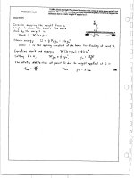
Example 6-1
1

A composite beam (Fig. 6-7) is constructed from a wood beam (4.0 in. ϫ 6.0 in.
actual dimensions) and a steel reinforcing plate (4.0 in. wide and 0.5 in. thick).
The wood and steel are securely fastened to act as a single beam. The beam is
subjected to a positive bending moment M ϭ 60 k-in.
Calculate the largest tensile and compressive stresses in the wood
(material 1) and the maximum and minimum tensile stresses in the steel (material 2) if E1 ϭ 1500 ksi and E2 ϭ 30,000 ksi.

y
A

h1

6 in.

Solution

z
h2
2

O
C

0.5 in.

B
4 in.

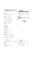
Neutral axis. The first step in the analysis is to locate the neutral axis of the
cross section. For that purpose, let us denote the distances from the neutral axis
to the top and bottom of the beam as h1 and h2, respectively. To obtain these
distances, we use Eq. (6-3). The integrals in that equation are evaluated by taking
the first moments of areas 1 and 2 about the z axis, as follows:

͵

FIG. 6-7 Example 6-1. Cross section of a
composite beam of wood and steel

͵

1

2

ydA ϭ ෆy1A1 ϭ (h1 Ϫ 3 in.)(4 in. ϫ 6 in.) ϭ (h1 Ϫ 3 in.)(24 in.2)

ydA ϭ ෆy2 A2 ϭ Ϫ(6.25 in. Ϫ h1)(4 in. ϫ 0.5 in.) ϭ (h1 Ϫ 6.25 in.)(2 in.2)

in which A1 and A2 are the areas of parts 1 and 2 of the cross section, ෆy1 and ෆy2 are
the y coordinates of the centroids of the respective areas, and h1 has units of inches.
Substituting the preceding expressions into Eq. (6-3) gives the equation for
locating the neutral axis, as follows:
E1

͵

1

ydA ϩ E2

͵

ydA ϭ 0

2

or
(1500 ksi)(h1 Ϫ 3 in.)(24 in.2) ϩ (30,000 ksi)(h1 Ϫ 6.25 in.)(2 in.2) ϭ 0
Solving this equation, we obtain the distance h1 from the neutral axis to the top
of the beam:
hl ϭ 5.031 in.
Also, the distance h2 from the neutral axis to the bottom of the beam is
h2 ϭ 6.5 in. Ϫ hl ϭ 1.469 in.
Thus, the position of the neutral axis is established.
Moments of inertia. The moments of inertia I1 and I2 of areas A1 and A2

with respect to the neutral axis can be found by using the parallel-axis theorem
(see Section 12.5 of Chapter 12). Beginning with area 1 (Fig. 6-7), we get
1
Il ϭ ᎏᎏ(4 in.)(6 in.) 3 ϩ (4 in.)(6 in.)(h1 Ϫ 3 in.) 2 ϭ 171.0 in.4
12


464

CHAPTER 6

Stresses in Beams (Advanced Topics)

Similarly, for area 2 we get
1
I2 ϭ ᎏᎏ(4 in.)(0.5 in.) 3 ϩ (4 in.)(0.5 in.)(h2 Ϫ 0.25 in.) 2 ϭ 3.01 in.4
12
To check these calculations, we can determine the moment of inertia I of the
entire cross-sectional area about the z axis as follows:
1
1
I ϭ ᎏᎏ(4 in.)h31 ϩ ᎏᎏ(4 in.)h 32 ϭ 169.8 ϩ 4.2 ϭ 174.0 in.4
3
3
which agrees with the sum of I1 and I2.
Normal stresses. The stresses in materials 1 and 2 are calculated from
the flexure formulas for composite beams (Eqs. 6-6a and b). The largest compressive stress in material 1 occurs at the top of the beam (A) where y ϭ h1 ϭ 5.031 in.
Denoting this stress by s1A and using Eq. (6-6a), we get
Mh1E1
s1A ϭ Ϫ ᎏᎏ

E1I1 ϩ E2I2
(60 k-in.)(5.031 in.)(1500 ksi)
ϭ Ϫ ᎏᎏᎏᎏᎏ
ϭ Ϫ1310 psi
(1500 ksi)(171.0 in.4) ϩ (30,000 ksi)(3.01 in.4)
The largest tensile stress in material 1 occurs at the contact plane between the
two materials (C) where y ϭ Ϫ(h2 Ϫ 0.5 in.) ϭ Ϫ0.969 in. Proceeding as in the
previous calculation, we get
(60 k-in.)(Ϫ0.969 in.)(1500 ksi)
ϭ 251 psi
s1C ϭ Ϫ ᎏᎏᎏᎏᎏ
(1500 ksi)(171.0 in.4) ϩ (30,000 ksi)(3.01 in.4)
Thus, we have found the largest compressive and tensile stresses in the wood.
The steel plate (material 2) is located below the neutral axis, and therefore
it is entirely in tension. The maximum tensile stress occurs at the bottom of the
beam (B) where y ϭ Ϫh2 ϭ Ϫ1.469 in. Hence, from Eq. (6-6b) we get
M(Ϫh2)E2
s2B ϭ Ϫ ᎏᎏ
E1I1 ϩ E2I2
(60 k-in.)(Ϫ1.469 in.)(30,000 ksi)
ϭ Ϫ ᎏᎏᎏᎏᎏ
ϭ 7620 psi
(1500 ksi)(171.0 in.4) ϩ (30,000 ksi)(3.01 in.4)
The minimum tensile stress in material 2 occurs at the contact plane (C) where
y ϭ Ϫ0.969 in. Thus,
(60 k-in.)(Ϫ0.969 in.)(30,000 ksi)
s2C ϭ Ϫ ᎏᎏᎏᎏᎏ
ϭ 5030 psi
(1500 ksi)(171.0 in.4) ϩ (30,000 ksi)(3.01 in.4)
These stresses are the maximum and minimum tensile stresses in the steel.

Note: At the contact plane the ratio of the stress in the steel to the stress in
the wood is
s2C /s1C ϭ 5030 psi/251 psi ϭ 20
which is equal to the ratio E2 /E1 of the moduli of elasticity (as expected).
Although the strains in the steel and wood are equal at the contact plane, the
stresses are different because of the different moduli.


SECTION 6.2

Composite Beams

465

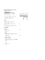
Example 6-2
A sandwich beam having aluminum-alloy faces enclosing a plastic core (Fig. 6-8)
is subjected to a bending moment M ϭ 3.0 kNиm. The thickness of the faces is
t ϭ 5 mm and their modulus of elasticity is E1 ϭ 72 GPa. The height of the plastic
core is hc ϭ 150 mm and its modulus of elasticity is E2 ϭ 800 MPa. The overall
dimensions of the beam are h ϭ 160 mm and b ϭ 200 mm.
Determine the maximum tensile and compressive stresses in the faces and
the core using: (a) the general theory for composite beams, and (b) the approximate theory for sandwich beams.
y
1
t = 5 mm
2
z
h
—
2

FIG. 6-8 Example 6-2. Cross section of
sandwich beam having aluminum-alloy
faces and a plastic core

O

hc =
150 mm

h=
160 mm

1

b = 200 mm

t = 5 mm

Solution
Neutral axis. Because the cross section is doubly symmetric, the neutral
axis (the z axis in Fig. 6-8) is located at midheight.
Moments of inertia. The moment of inertia I1 of the cross-sectional areas of
the faces (about the z axis) is

΄

΅

b

200 mm
I1 ϭ ᎏᎏ(h3 Ϫ h3c ) ϭ ᎏᎏ (160 mm)3 Ϫ (150 mm)3 ϭ 12.017 ϫ 106 mm4
12
12
and the moment of inertia I2 of the plastic core is
b
200 mm
I2 ϭ ᎏᎏ(h3c) ϭ ᎏᎏ (150 mm)3 ϭ 56.250 ϫ 106 mm4
12
12
As a check on these results, note that the moment of inertia of the entire crosssectional area about the z axis (I ϭ bh3/12) is equal to the sum of I1 and I2.
(a) Normal stresses calculated from the general theory for composite beams.
To calculate these stresses, we use Eqs. (6-6a) and (6-6b). As a preliminary
matter, we will evaluate the term in the denominator of those equations (that is,
the flexural rigidity of the composite beam):
E1I1 ϩ E2I2 ϭ (72 GPa)(12.017 ϫ 106 mm4) ϩ (800 MPa)(56.250 ϫ 106 mm4)
ϭ 910,200 Nиm2


466

CHAPTER 6

Stresses in Beams (Advanced Topics)

The maximum tensile and compressive stresses in the aluminum faces are found
from Eq. (6-6a):
M(h/2)(E1)
(s 1)max ϭ Ϯ ᎏᎏ
E1I1 ϩ E2I2

(3.0 kNиm)(80 mm)(72 GPa)
ϭ Ϯ ᎏᎏᎏ
ϭ Ϯ 19.0 MPa
910,200 Nиm2
The corresponding quantities for the plastic core (from Eq. 6-6b) are
M(hc /2)(E2)
(s2)max ϭ Ϯ ᎏᎏ
E1I1 ϩ E2I2
(3.0 kNиm)(75 mm)(800 MPa)
ϭ Ϯ ᎏᎏᎏᎏ
ϭ Ϯ 0.198 MPa
910,200 Nиm2
The maximum stresses in the faces are 96 times greater than the maximum
stresses in the core, primarily because the modulus of elasticity of the aluminum
is 90 times greater than that of the plastic.
(b) Normal stresses calculated from the approximate theory for sandwich
beams. In the approximate theory we disregard the normal stresses in the core
and assume that the faces transmit the entire bending moment. Then the
maximum tensile and compressive stresses in the faces can be found from
Eqs. (6-9a) and (6-9b), as follows:
(3.0 kNиm)(80 mm)
Mh
ϭ Ϯ 20.0 MPa
(s1)max ϭ Ϯ ᎏᎏ ϭ Ϯ ᎏᎏᎏ
2I1
12.017 ϫ 106 mm4
As expected, the approximate theory gives slightly higher stresses in the faces
than does the general theory for composite beams.

6.3 TRANSFORMED-SECTION METHOD

The transformed-section method is an alternative procedure for analyzing the bending stresses in a composite beam. The method is based upon
the theories and equations developed in the preceding section, and
therefore it is subject to the same limitations (for instance, it is valid
only for linearly elastic materials) and gives the same results. Although
the transformed-section method does not reduce the calculating effort,
many designers find that it provides a convenient way to visualize and
organize the calculations.
The method consists of transforming the cross section of a composite beam into an equivalent cross section of an imaginary beam that is
composed of only one material. This new cross section is called the


SECTION 6.3

Transformed-Section Method

467

transformed section. Then the imaginary beam with the transformed
section is analyzed in the customary manner for a beam of one material.
As a final step, the stresses in the transformed beam are converted to
those in the original beam.

Neutral Axis and Transformed Section

b1
y

If the transformed beam is to be equivalent to the original beam, its neutral axis must be located in the same place and its moment-resisting
capacity must be the same. To show how these two requirements are
met, consider again a composite beam of two materials (Fig. 6-9a). The

neutral axis of the cross section is obtained from Eq. (6-3), which is
repeated here:

1

E1

͵

ydA ϩ E2

1

z
2

O
b2
(a)

E2
n ϭ ᎏᎏ
E1

y

(6-11)

(6-12)

where n is the modular ratio. With this notation, we can rewrite Eq. (6-11)
in the form

1

1

ydA ϭ 0

2

In this equation, the integrals represent the first moments of the two
parts of the cross section with respect to the neutral axis.
Let us now introduce the notation

b1

z

͵

O
nb2
(b)

FIG. 6-9 Composite beam of two

materials: (a) actual cross section, and
(b) transformed section consisting only
of material 1

͵

1

y dA ϩ

͵

yn dA ϭ 0

(6-13)

2

Since Eqs. (6-11) and (6-13) are equivalent, the preceding equation
shows that the neutral axis is unchanged if each element of area dA in
material 2 is multiplied by the factor n, provided that the y coordinate
for each such element of area is not changed.
Therefore, we can create a new cross section consisting of two
parts: (1) area 1 with its dimensions unchanged, and (2) area 2 with
its width (that is, its dimension parallel to the neutral axis) multiplied
by n. This new cross section (the transformed section) is shown in
Fig. 6-9b for the case where E2 Ͼ E1 (and therefore n Ͼ 1). Its neutral axis is in the same position as the neutral axis of the original
beam. (Note that all dimensions perpendicular to the neutral axis
remain the same.)
Since the stress in the material (for a given strain) is proportional to
the modulus of elasticity (s ϭ Ee), we see that multiplying the width of
material 2 by n ϭ E2 /E1 is equivalent to transforming it to material 1.
For instance, suppose that n ϭ 10. Then the area of part 2 of the cross

section is now 10 times wider than before. If we imagine that this part of


468

CHAPTER 6

Stresses in Beams (Advanced Topics)

the beam is now material 1, we see that it will carry the same force as
before because its modulus is reduced by a factor of 10 (from E2 to E1)
at the same time that its area is increased by a factor of 10. Thus, the
new section (the transformed section) consists only of material 1.

Moment-Curvature Relationship
The moment-curvature relationship for the transformed beam must be
the same as for the original beam. To show that this is indeed the case,
we note that the stresses in the transformed beam (since it consists only
of material 1) are given by Eq. (5-7) of Section 5.5:
sx ϭ ϪE1ky
Using this equation, and also following the same procedure as for a
beam of one material (see Section 5.5), we can obtain the momentcurvature relation for the transformed beam:

͵
͵

͵
͵

sxy dA ϭ Ϫ

MϭϪ

A

ϭ E1k

1

sxy dA Ϫ

1

y2 dA ϩ E1k

͵

sxy dA

2

y 2 dA ϭ k(E1I1 ϩ E1 nI2)

2

or
M ϭ k(E1 I1 ϩ E2 I2)

(6-14)

This equation is the same as Eq. (6-4), thereby demonstrating that the
moment-curvature relationship for the transformed beam is the same as
for the original beam.

Normal Stresses
Since the transformed beam consists of only one material, the normal
stresses (or bending stresses) can be found from the standard flexure
formula (Eq. 5-13). Thus, the normal stresses in the beam transformed to
material 1 (Fig. 6-9b) are
My
sx1 ϭ Ϫ ᎏᎏ
IT

(6-15)

where IT is the moment of inertia of the transformed section with respect
to the neutral axis. By substituting into this equation, we can calculate the
stresses at any point in the transformed beam. (As explained later,
the stresses in the transformed beam match those in the original beam
in the part of the original beam consisting of material 1; however, in the
part of the original beam consisting of material 2, the stresses are different from those in the transformed beam.)


SECTION 6.3

Transformed-Section Method

469

We can easily verify Eq. (6-15) by noting that the moment of inertia

of the transformed section (Fig. 6-9b) is related to the moment of inertia
of the original section (Fig. 6-9a) by the following relation:
E2
IT ϭ I1 ϩ nI2 ϭ I1 ϩ ᎏᎏ I2
E1

(6-16)

Substituting this expression for IT into Eq. (6-15) gives
MyE1
sx1 ϭ Ϫ ᎏᎏ
E1I1 ϩ E2I2

(a)

which is the same as Eq. (6-6a), thus demonstrating that the stresses in
material 1 in the original beam are the same as the stresses in the corresponding part of the transformed beam.
As mentioned previously, the stresses in material 2 in the original
beam are not the same as the stresses in the corresponding part of
the transformed beam. Instead, the stresses in the transformed beam
(Eq. 6-15) must be multiplied by the modular ratio n to obtain the
stresses in material 2 of the original beam:
My
sx 2 ϭ Ϫ ᎏᎏ n
IT

(6-17)

We can verify this formula by noting that when Eq. (6-16) for IT is substituted into Eq. (6-17), we get
MyE2

MynE1
sx 2 ϭ Ϫ ᎏᎏ ϭ Ϫ ᎏᎏ
E1I1 ϩ E2I2
E1I1 ϩ E2I2

(b)

which is the same as Eq. (6-6b).

General Comments
In this discussion of the transformed-section method we chose to transform the original beam to a beam consisting entirely of material 1. It
is also possible to transform the beam to material 2. In that case the
stresses in the original beam in material 2 will be the same as the
stresses in the corresponding part of the transformed beam. However,
the stresses in material 1 in the original beam must be obtained by
multiplying the stresses in the corresponding part of the transformed
beam by the modular ratio n, which in this case is defined as
n ϭ E1/E2.
It is also possible to transform the original beam into a material having any arbitrary modulus of elasticity E, in which case all parts of the
beam must be transformed to the fictitious material. Of course, the calculations are simpler if we transform to one of the original materials.
Finally, with a little ingenuity it is possible to extend the transformedsection method to composite beams of more than two materials.


470

CHAPTER 6

Stresses in Beams (Advanced Topics)

Example 6-3

The composite beam shown in Fig. 6-10a is formed of a wood beam (4.0 in. ϫ 6.0
in. actual dimensions) and a steel reinforcing plate (4.0 in. wide and 0.5 in. thick).
The beam is subjected to a positive bending moment M ϭ 60 k-in.
Using the transformed-section method, calculate the largest tensile and
compressive stresses in the wood (material 1) and the maximum and minimum
tensile stresses in the steel (material 2) if E1 ϭ 1500 ksi and E2 ϭ 30,000 ksi.
Note: This same beam was analyzed previously in Example 6-1 of Section 6.2.
1

y

1

4 in.

A

A

y
h1

FIG. 6-10 Example 6-3. Composite

beam of Example 6-1 analyzed by the
transformed-section method:
(a) cross section of original beam, and
(b) transformed section (material 1)

z

h2
2

h1

6 in.

O
4 in.

z

C
B

6 in.
0.5 in.
O

h2

80 in.

0.5 in.
1

(a)

C
B

(b)

Solution
Transformed section. We will transform the original beam into a beam of
material 1, which means that the modular ratio is defined as
E2
30,000 ksi
n ϭ ᎏᎏ ϭ ᎏᎏ ϭ 20
E1
1,500 ksi
The part of the beam made of wood (material 1) is not altered but the part made
of steel (material 2) has its width multiplied by the modular ratio. Thus, the width
of this part of the beam becomes
n(4 in.) ϭ 20(4 in.) ϭ 80 in.
in the transformed section (Fig. 6-10b).
Neutral axis. Because the transformed beam consists of only one material,
the neutral axis passes through the centroid of the cross-sectional area. Therefore,
with the top edge of the cross section serving as a reference line, and with the
distance yi measured positive downward, we can calculate the distance h1 to the
centroid as follows:
(3 in.)(4 in.)(6 in.) ϩ (6.25 in.)(80 in.)(0.5 in.)
Αyi Ai
h1 ϭ ᎏᎏ ϭ ᎏᎏᎏᎏᎏ
(4 in.)(6 in.) ϩ (80 in.)(0.5 in.)
ΑAi
322.0 in.3
ϭ 5.031 in.
ϭ ᎏᎏ
64.0 in.2

continued


SECTION 6.3

Transformed-Section Method

471

Also, the distance h2 from the lower edge of the section to the centroid is
h 2 ϭ 6.5 in. Ϫ h1 ϭ 1.469 in.
Thus, the location of the neutral axis is determined.
Moment of inertia of the transformed section. Using the parallel-axis
theorem (see Section 12.5 of Chapter 12), we can calculate the moment of
inertia IT of the entire cross-sectional area with respect to the neutral axis as
follows:
1
IT ϭ ᎏᎏ(4 in.)(6 in.)3 ϩ (4 in.)(6 in.)(h1 Ϫ 3 in.) 2
12
1
ϩ ᎏᎏ(80 in.)(0.5 in.)3 ϩ (80 in.)(0.5 in.)(h2 Ϫ 0.25 in.) 2
12
ϭ 171.0 in.4 ϩ 60.3 in.4 ϭ 231.3 in.4

1

Normal stresses in the wood (material 1). The stresses in the transformed
beam (Fig. 6-10b) at the top of the cross section (A) and at the contact plane
between the two parts (C) are the same as in the original beam (Fig. 6-10a).
These stresses can be found from the flexure formula (Eq. 6-15), as follows:

y
A

(60 k-in.)(5.031 in.)
My
ϭ Ϫ1310 psi
s1A ϭ Ϫ ᎏᎏ ϭ Ϫ ᎏᎏᎏ
231.3 in.4
IT
h1

6 in.

z
h2
2

O

(60 k-in.)(Ϫ0.969 in.)
My
s1C ϭ Ϫ ᎏᎏ ϭ Ϫ ᎏᎏᎏ
ϭ 251 psi
231.3 in.4
IT

C
B

4 in.

0.5 in.

(a)
1

4 in.

A

y
h1

z

(60 k-in.)(Ϫ1.469 in.)
My
(20) ϭ 7620 psi
s2B ϭ Ϫ ᎏᎏn ϭ Ϫ ᎏᎏᎏ
231.3 in.4
IT

6 in.
0.5 in.
O

h2

80 in.

1

(b)

FIG. 6-10 (Repeated)

These are the largest tensile and compressive stresses in the wood (material 1)
in the original beam. The stress s1A is compressive and the stress s1C is
tensile.
Normal stresses in the steel (material 2). The maximum and minimum
stresses in the steel plate are found by multiplying the corresponding stresses in
the transformed beam by the modular ratio n (Eq. 6-17). The maximum stress
occurs at the lower edge of the cross section (B) and the minimum stress occurs
at the contact plane (C ):

C
B

(60 k-in.)(Ϫ0.969 in.)
My
s2C ϭ Ϫ ᎏᎏn ϭ Ϫ ᎏᎏᎏ
(20) ϭ 5030 psi
231.3 in.4
IT
Both of these stresses are tensile.
Note that the stresses calculated by the transformed-section method agree
with those found in Example 6-1 by direct application of the formulas for a composite beam.


472

CHAPTER 6

Stresses in Beams (Advanced Topics)

6.4 DOUBLY SYMMETRIC BEAMS WITH INCLINED LOADS
y

z

x
FIG. 6-11 Beam with a lateral load acting
in a plane of symmetry

y

In our previous discussions of bending we dealt with beams possessing a
longitudinal plane of symmetry (the xy plane in Fig. 6-11) and supporting lateral loads acting in that same plane. Under these conditions the
bending stresses can be obtained from the flexure formula (Eq. 5-13)
provided the material is homogeneous and linearly elastic.
In this section, we will extend those ideas and consider what happens when the beam is subjected to loads that do not act in the plane of
symmetry, that is, inclined loads (Fig. 6-12). We will limit our discussion to beams that have a doubly symmetric cross section, that is, both
the xy and xz planes are planes of symmetry. Also, the inclined loads
must act through the centroid of the cross section to avoid twisting the
beam about the longitudinal axis.
We can determine the bending stresses in the beam shown in
Fig. 6-12 by resolving the inclined load into two components, one acting
in each plane of symmetry. Then the bending stresses can be obtained
from the flexure formula for each load component acting separately, and
the final stresses can be obtained by superposing the separate stresses.

Sign Conventions for Bending Moments
z

x
FIG. 6-12 Doubly symmetric beam with

an inclined load

y

My

Normal Stresses (Bending Stresses)
The normal stresses associated with the individual bending moments My
and Mz are obtained from the flexure formula (Eq. 5-13). These stresses

Mz
z

As a preliminary matter, we will establish sign conventions for the bending moments acting on cross sections of a beam.* For this purpose, we
cut through the beam and consider a typical cross section (Fig. 6-13).
The bending moments My and Mz acting about the y and z axes, respectively, are represented as vectors using double-headed arrows. The
moments are positive when their vectors point in the positive directions
of the corresponding axes, and the right-hand rule for vectors gives the
direction of rotation (indicated by the curved arrows in the figure).
From Fig. 6-13 we see that a positive bending moment My produces
compression on the right-hand side of the beam (the negative z side) and
tension on the left-hand side (the positive z side). Similarly, a positive
moment Mz produces compression on the upper part of the beam (where y

is positive) and tension on the lower part (where y is negative). Also, it is
important to note that the bending moments shown in Fig. 6-13 act on the
positive x face of a segment of the beam, that is, on a face having its outward normal in the positive direction of the x axis.

x
*

FIG. 6-13 Sign conventions for bending

moments My and Mz

The directions of the normal and shear stresses in a beam are usually apparent from an
inspection of the beam and its loading, and therefore we often calculate stresses by ignoring
sign conventions and using only absolute values. However, when deriving general formulas
we need to maintain rigorous sign conventions to avoid ambiguity in the equations.


SECTION 6.4

n

z

My

y

z

Mz

473

are then superposed to give the stresses produced by both moments acting simultaneously. For instance, consider the stresses at a point in the
cross section having positive coordinates y and z (point A in Fig. 6-14).
A positive moment My produces tension at this point and a positive
moment Mz produces compression; thus, the normal stress at point A is

y

A
b

Doubly Symmetric Beams with Inclined Loads

C

My z
Mz y
sx ϭ ᎏᎏ Ϫ ᎏᎏ
Iy
Iz
n

(6-18)

in which Iy and Iz are the moments of inertia of the cross-sectional area
with respect to the y and z axes, respectively. Using this equation, we
can find the normal stress at any point in the cross section by substituting the appropriate algebraic values of the moments and the coordinates.

FIG. 6-14 Cross section of beam

subjected to bending moments My
and Mz

Neutral Axis
The equation of the neutral axis can be determined by equating the normal stress sx (Eq. 6-18) to zero:

y

My
Mz
ᎏᎏz Ϫ ᎏᎏy ϭ 0
Iy
Iz

L-x

(6-19)

L
u
z
P

(a)

x

n

y
u

b

u
z

MyIz
y
tan b ϭ ᎏᎏ ϭ ᎏᎏ
MzIy
z

(6-20)

Depending upon the magnitudes and directions of the bending moments,
the angle b may vary from Ϫ90° to ϩ90°. Knowing the orientation of
the neutral axis is useful when determining the points in the cross section where the normal stresses are the largest. (Since the stresses vary
linearly with distance from the neutral axis, the maximum stresses occur
at points located farthest from the neutral axis.)

P

My

M

This equation shows that the neutral axis nn is a straight line passing

through the centroid C (Fig. 6-14). The angle b between the neutral axis
and the z axis is determined as follows:

C

Mz

Relationship Between the Neutral Axis
and the Inclination of the Loads
n
(b)
FIG. 6-15 Doubly symmetric beam with
an inclined load P acting at an angle u
to the positive y axis

As we have just seen, the orientation of the neutral axis with respect to
the z axis is determined by the bending moments and the moments of
inertia (Eq. 6-20). Now we wish to determine the orientation of the neutral axis relative to the angle of inclination of the loads acting on the
beam. For this purpose, we will use the cantilever beam shown in
Fig. 6-15a as an example. The beam is loaded by a force P acting in the


474

CHAPTER 6

Stresses in Beams (Advanced Topics)

plane of the end cross section and inclined at an angle u to the positive y
axis. This particular orientation of the load is selected because it means

that both bending moments (My and Mz) are positive when u is between
0 and 90°.
The load P can be resolved into components P cos u in the positive y
direction and P sin u in the negative z direction. Therefore, the bending
moments My and Mz (Fig. 6-15b) acting on a cross section located at distance x from the fixed support are
My ϭ (P sin u )(L Ϫ x)

Mz ϭ (P cos u)(L Ϫ x)

(6-21a,b)

in which L is the length of the beam. The ratio of these moments is
My
(6-22)
ᎏ ϭ tan u
Mz
which shows that the resultant moment vector M is at the angle u from
the z axis (Fig. 6-15b). Consequently, the resultant moment vector is
perpendicular to the longitudinal plane containing the force P.
The angle b between the neutral axis nn and the z axis (Fig. 6-15b)
is obtained from Eq. (6-20):
My Iz
Iz
tan b ϭ ᎏ ϭ ᎏᎏ tan u
MzIy
Iy

(6-23)

which shows that the angle b is generally not equal to the angle u. Thus,

except in special cases, the neutral axis is not perpendicular to the
longitudinal plane containing the load.
Exceptions to this general rule occur in three special cases:
1. When the load lies in the xy plane (u ϭ 0 or 180°), which means
that the z axis is the neutral axis.
2. When the load lies in the xz plane (u ϭ Ϯ 90°), which means that
the y axis is the neutral axis.
3. When the principal moments of inertia are equal, that is, when
Iy ϭ Iz.
In case (3), all axes through the centroid are principal axes and all
have the same moment of inertia. The plane of loading, no matter what
its direction, is always a principal plane, and the neutral axis is always
perpendicular to it. (This situation occurs with square, circular, and certain other cross sections, as described in Section 12.9 of Chapter 12.)
The fact that the neutral axis is not necessarily perpendicular to the
plane of the load can greatly affect the stresses in a beam, especially if
the ratio of the principal moments of inertia is very large. Under these
conditions the stresses in the beam are very sensitive to slight changes in
the direction of the load and to irregularities in the alignment of the
beam itself. This characteristic of certain beams is illustrated later in
Example 6-5.


SECTION 6.4

Doubly Symmetric Beams with Inclined Loads

475

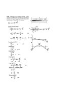
Example 6-4
A wood beam AB of rectangular cross section serving as a roof purlin (Figs. 6-16a

and b) is simply supported by the top chords of two adjacent roof trusses. The
beam supports the weight of the roof sheathing and the roofing material, plus its
own weight and any additional loads that affect the roof (such as wind, snow, and
earthquake loads).
In this example, we will consider only the effects of a uniformly distributed
load of intensity q ϭ 3.0 kN/m acting in the vertical direction through the centroids of the cross sections (Fig. 6-16c). The load acts along the entire length of
the beam and includes the weight of the beam. The top chords of the trusses have
a slope of 1 on 2 (a ϭ 26.57°), and the beam has width b ϭ 100 mm, height
h ϭ 150 mm, and span L ϭ 1.6 m.
Determine the maximum tensile and compressive stresses in the beam and
locate the neutral axis.

Roof
sheathing

y

A
a

A

b
B

Purlin
Roof truss

z

L

a

rectangular cross section serving as a
roof purlin

C
q
2
a = 26.57°

1

(c)

(b)

(a)
FIG. 6-16 Example 6-4. Wood beam of

h

a

B

Solution
Loads and bending moments. The uniform load q acting in the vertical
direction can be resolved into components in the y and z directions (Fig. 6-17a):

qy ϭ q cos a

qz ϭ q sin a

(6-24a,b)

The maximum bending moments occur at the midpoint of the beam and are
found from the general formula M ϭ qL2/8; hence,
qz L2
qL2sin a
My ϭ ᎏᎏ ϭ ᎏᎏ
8
8

qy L2
qL2cos a
Mz ϭ ᎏ ϭ ᎏᎏ
8
8

(6-25a,b)

Both of these moments are positive because their vectors are in the positive
directions of the y and z axes (Fig. 6-17b).
Moments of inertia. The moments of inertia of the cross-sectional area with
respect to the y and z axes are as follows:
hb3
Iy ϭ ᎏᎏ
12

bh3
Iz ϭ ᎏᎏ
12

(6-26a,b)

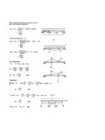
Bending stresses. The stresses at the midsection of the beam are obtained
from Eq. (6-18) with the bending moments given by Eqs. (6-25) and the moments
of inertia given by Eqs. (6-26):


476

CHAPTER 6

Stresses in Beams (Advanced Topics)

My z
Mz y
qL2sin a
qL2cos a
sx ϭ ᎏ Ϫ ᎏᎏ ϭ ᎏ3ᎏ z Ϫ ᎏ3ᎏy
Iy
Iz
8hb /12
8bh /12
y

3qL2 sin a
cos a

Ϫ ᎏᎏy
ϭ ᎏᎏ ᎏᎏz
2bh b2
h2

΂

D

E

qy

a

q
(a)

3qL2 sin a
cos a
sE ϭ ϪsD ϭ ᎏᎏ ᎏᎏ ϩ ᎏᎏ
b
h
4bh

΂

y
n

q ϭ 3.0 kN/m

My
b

h
C
Mz

E

n
b

a

(6-28)

L ϭ 1.6 m

b ϭ 100 mm

h ϭ 150 mm

␣ ϭ 26.57°

The results are

a
z

΃

Numerical values. The maximum tensile and compressive stresses can be
calculated from the preceding equation by substituting the given data:

D

M

(6-27)

The stress at any point in the cross section can be obtained from this equation by
substituting the coordinates y and z of the point.
From the orientation of the cross section and the directions of the loads and
bending moments (Fig. 6-17), it is apparent that the maximum compressive
stress occurs at point D (where y ϭ h/2 and z ϭ Ϫb/2) and the maximum tensile
stress occurs at point E (where y ϭ Ϫh/2 and z ϭ b/2). Substituting these coordinates into Eq. (6-27) and then simplifying, we obtain expressions for the maximum and minimum stresses in the beam:

C
a

qz
z

΃

sE ϭ ϪsD ϭ 4.01 MPa
Neutral axis. In addition to finding the stresses in the beam, it is often
useful to locate the neutral axis. The equation of this line is obtained by setting

the stress (Eq. 6-27) equal to zero:

(b)

sin a
cos a
ᎏᎏ
z Ϫ ᎏᎏ
yϭ0
b2
h2
y

(6-29)

The neutral axis is shown in Fig. 6-17b as line nn. The angle b from the z axis to
the neutral axis is obtained from Eq. (6-29) as follows:
D 4.01 MPa

0.57 MPa
n

y
h2
tan b ϭ ᎏᎏ ϭ ᎏᎏ2 tan a
b
z

(6-30)

Substituting numerical values, we get

b
n
z

x

E
4.01 MPa

0.57 MPa
(c)

FIG. 6-17 Solution to Example 6-4.

(a) Components of the uniform load, (b)
bending moments acting on a cross section, and (c) Normal stress distribution

΂

΃

(150 mm)2
h2
tan b ϭ ᎏᎏ2 tan a ϭ ᎏᎏ2 tan 26.57° ϭ 1.125
b
(100 mm)

b ϭ 48.4°

Since the angle b is not equal to the angle a, the neutral axis is inclined to the
plane of loading (which is vertical).
From the orientation of the neutral axis (Fig. 6-17b), we see that points D
and E are the farthest from the neutral axis, thus confirming our assumption that
the maximum stresses occur at those points. The part of the beam above and
to the right of the neutral axis is in compression, and the part to the left and below
the neutral axis is in tension.


SECTION 6.4

477

Doubly Symmetric Beams with Inclined Loads

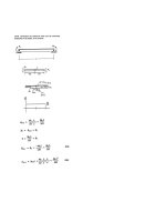
Example 6-5
A 12-foot long cantilever beam (Fig. 6-18a) is constructed from an S 24 ϫ 80
section (see Table E-2 of Appendix E for the dimensions and properties of this
beam). A load P ϭ 10 k acts in the vertical direction at the end of the beam.
Because the beam is very narrow compared to its height (Fig. 6-18b), its
moment of inertia about the z axis is much larger than its moment of inertia about
the y axis.
(a) Determine the maximum bending stresses in the beam if the y axis
of the cross section is vertical and therefore aligned with the load P (Fig. 6-18a).
(b) Determine the maximum bending stresses if the beam is inclined at a
small angle a ϭ 1° to the load P (Fig. 6-18b). (A small inclination can be caused
by imperfections in the fabrication of the beam, misalignment of the beam during
construction, or movement of the supporting structure.)

y

y

L = 12 ft
z

A

n

b = 41°
C

z

C

n
S 24 ϫ 80

B

x
FIG. 6-18 Example 6-5. Cantilever beam

P

P = 10 k

with moment of inertia Iz much larger
than Iy

a = 1°
(b)

(a)

Solution
(a) Maximum bending stresses when the load is aligned with the y axis. If
the beam and load are in perfect alignment, the z axis is the neutral axis and the
maximum stresses in the beam (at the support) are obtained from the flexure
formula:
My
PL(h/2)
smax ϭ ᎏᎏ ϭ ᎏᎏ
Iz
Iz
in which Mz ϭ ϪM ϭ ϪPL and My ϭ 0 so M ϭ PL is the bending moment at
the support, h is the height of the beam, and Iz is the moment of inertia about the
z axis. Substituting numerical values, we obtain
(10 k)(12 ft)(12 in./ft)(12.00 in.)
smax ϭ ᎏᎏᎏᎏ
ϭ 8230 psi
2100 in.4
This stress is tensile at the top of the beam and compressive at the bottom of the
beam.


478

CHAPTER 6

Stresses in Beams (Advanced Topics)

(b) Maximum bending stresses when the load is inclined to the y axis. We
now assume that the beam has a small inclination (Fig. 6-18b), so that the angle
between the y axis and the load is a ϭ 1°.
The components of the load P are P cos a in the negative y direction and
P sin a in the positive z direction. Therefore, the bending moments at the
support are
My ϭ Ϫ(P sin a)L ϭ Ϫ(10 k)(sin 1°)(12 ft)(12 in./ft) ϭ Ϫ25.13 k-in.
Mz ϭ Ϫ(P cos a)L ϭ Ϫ(10 k)(cos 1°)(12 ft)(12 in./ft) ϭ Ϫ1440 k-in.
The angle b giving the orientation of the neutral axis nn (Fig. 6-18b) is obtained
from Eq. (6-20):
My Iz
y
(Ϫ25.13 k-in.)(2100 in.4)
ϭ 0.8684
tan b ϭ ᎏᎏ ϭ ᎏ ϭ ᎏᎏᎏ
MzIy
z
(Ϫ1440 k-in.)(42.2 in.4)

b ϭ 41°

This calculation shows that the neutral axis is inclined at an angle of 41° from
the z axis even though the plane of the load is inclined only 1° from the y axis.
The sensitivity of the position of the neutral axis to the angle of the load is a consequence of the large Iz /Iy ratio.
From the position of the neutral axis (Fig. 6-18b), we see that the maximum

stresses in the beam occur at points A and B, which are located at the farthest distances from the neutral axis. The coordinates of point A are
zA ϭ Ϫ3.50 in.

yA ϭ 12.0 in.

Therefore, the tensile stress at point A (see Eq. 6-18) is
My zA
Mz yA
sA ϭ ᎏ Ϫ ᎏᎏ
Iy
Iz
(Ϫ1440 k-in.)(12.0 in.)
(Ϫ25.13 k-in.)(Ϫ3.50 in.)
ϭ ᎏᎏᎏ
Ϫ ᎏᎏᎏ
2100 in.4
42.2 in.4
ϭ 2080 psi ϩ 8230 psi ϭ 10,310 psi
The stress at B has the same magnitude but is a compressive stress:
sB ϭ Ϫ10,310 psi
These stresses are 25% larger than the stress smax ϭ 8230 psi for the same
beam with a perfectly aligned load. Furthermore, the inclined load produces a
lateral deflection in the z direction, whereas the perfectly aligned load does not.
This example shows that beams with Iz much larger than Iy may develop
large stresses if the beam or its loads deviate even a small amount from their
planned alignment. Therefore, such beams should be used with caution, because
they are highly susceptible to overstress and to lateral (that is, sideways)
bending and buckling. The remedy is to provide adequate lateral support for
the beam, thereby preventing sideways bending. For instance, wood floor joists
in buildings are supported laterally by installing bridging or blocking between

the joists.