The elements of statistical LEarning data mininb 2nd
Bạn đang xem bản rút gọn của tài liệu. Xem và tải ngay bản đầy đủ của tài liệu tại đây (12.69 MB, 764 trang )
Trevor Hastie • Robert Tibshirani • Jerome Friedman
The Elements of Statictical Learning
This major new edition features many topics not covered in the original, including graphical
models, random forests, ensemble methods, least angle regression & path algorithms for the
lasso, non-negative matrix factorization, and spectral clustering. There is also a chapter on
methods for “wide” data (p bigger than n), including multiple testing and false discovery rates.
Trevor Hastie, Robert Tibshirani, and Jerome Friedman are professors of statistics at
Stanford University. They are prominent researchers in this area: Hastie and Tibshirani
developed generalized additive models and wrote a popular book of that title. Hastie codeveloped much of the statistical modeling software and environment in R/S-PLUS and
invented principal curves and surfaces. Tibshirani proposed the lasso and is co-author of the
very successful An Introduction to the Bootstrap. Friedman is the co-inventor of many datamining tools including CART, MARS, projection pursuit and gradient boosting.
S TAT I S T I C S
----
› springer.com
The Elements of Statistical Learning
During the past decade there has been an explosion in computation and information technology. With it have come vast amounts of data in a variety of fields such as medicine, biology, finance, and marketing. The challenge of understanding these data has led to the development of new tools in the field of statistics, and spawned new areas such as data mining,
machine learning, and bioinformatics. Many of these tools have common underpinnings but
are often expressed with different terminology. This book describes the important ideas in
these areas in a common conceptual framework. While the approach is statistical, the
emphasis is on concepts rather than mathematics. Many examples are given, with a liberal
use of color graphics. It should be a valuable resource for statisticians and anyone interested
in data mining in science or industry. The book’s coverage is broad, from supervised learning
(prediction) to unsupervised learning. The many topics include neural networks, support
vector machines, classification trees and boosting—the first comprehensive treatment of this
topic in any book.
Hastie • Tibshirani • Friedman
Springer Series in Statistics
Springer Series in Statistics
Trevor Hastie
Robert Tibshirani
Jerome Friedman
The Elements of
Statistical Learning
Data Mining, Inference, and Prediction
Second Edition
This is page v
Printer: Opaque this
To our parents:
Valerie and Patrick Hastie
Vera and Sami Tibshirani
Florence and Harry Friedman
and to our families:
Samantha, Timothy, and Lynda
Charlie, Ryan, Julie, and Cheryl
Melanie, Dora, Monika, and Ildiko
vi
This is page vii
Printer: Opaque this
Preface to the Second Edition
In God we trust, all others bring data.
–William Edwards Deming (1900-1993)1
We have been gratified by the popularity of the first edition of The
Elements of Statistical Learning. This, along with the fast pace of research
in the statistical learning field, motivated us to update our book with a
second edition.
We have added four new chapters and updated some of the existing
chapters. Because many readers are familiar with the layout of the first
edition, we have tried to change it as little as possible. Here is a summary
of the main changes:
1 On the Web, this quote has been widely attributed to both Deming and Robert W.
Hayden; however Professor Hayden told us that he can claim no credit for this quote,
and ironically we could find no “data” confirming that Deming actually said this.
viii
Preface to the Second Edition
Chapter
1. Introduction
2. Overview of Supervised Learning
3. Linear Methods for Regression
4. Linear Methods for Classification
5. Basis Expansions and Regularization
6. Kernel Smoothing Methods
7. Model Assessment and Selection
8. Model Inference and Averaging
9. Additive Models, Trees, and
Related Methods
10. Boosting and Additive Trees
11. Neural Networks
12. Support Vector Machines and
Flexible Discriminants
13.
Prototype
Methods
and
Nearest-Neighbors
14. Unsupervised Learning
15.
16.
17.
18.
Random Forests
Ensemble Learning
Undirected Graphical Models
High-Dimensional Problems
What’s new
LAR algorithm and generalizations
of the lasso
Lasso path for logistic regression
Additional illustrations of RKHS
Strengths and pitfalls of crossvalidation
New example from ecology; some
material split off to Chapter 16.
Bayesian neural nets and the NIPS
2003 challenge
Path algorithm for SVM classifier
Spectral clustering, kernel PCA,
sparse PCA, non-negative matrix
factorization archetypal analysis,
nonlinear
dimension
reduction,
Google page rank algorithm, a
direct approach to ICA
New
New
New
New
Some further notes:
• Our first edition was unfriendly to colorblind readers; in particular,
we tended to favor red/green contrasts which are particularly troublesome. We have changed the color palette in this edition to a large
extent, replacing the above with an orange/blue contrast.
• We have changed the name of Chapter 6 from “Kernel Methods” to
“Kernel Smoothing Methods”, to avoid confusion with the machinelearning kernel method that is discussed in the context of support vector machines (Chapter 11) and more generally in Chapters 5 and 14.
• In the first edition, the discussion of error-rate estimation in Chapter 7 was sloppy, as we did not clearly differentiate the notions of
conditional error rates (conditional on the training set) and unconditional rates. We have fixed this in the new edition.
Preface to the Second Edition
ix
• Chapters 15 and 16 follow naturally from Chapter 10, and the chapters are probably best read in that order.
• In Chapter 17, we have not attempted a comprehensive treatment
of graphical models, and discuss only undirected models and some
new methods for their estimation. Due to a lack of space, we have
specifically omitted coverage of directed graphical models.
• Chapter 18 explores the “p ≫ N ” problem, which is learning in highdimensional feature spaces. These problems arise in many areas, including genomic and proteomic studies, and document classification.
We thank the many readers who have found the (too numerous) errors in
the first edition. We apologize for those and have done our best to avoid errors in this new edition. We thank Mark Segal, Bala Rajaratnam, and Larry
Wasserman for comments on some of the new chapters, and many Stanford
graduate and post-doctoral students who offered comments, in particular
Mohammed AlQuraishi, John Boik, Holger Hoefling, Arian Maleki, Donal
McMahon, Saharon Rosset, Babak Shababa, Daniela Witten, Ji Zhu and
Hui Zou. We thank John Kimmel for his patience in guiding us through this
new edition. RT dedicates this edition to the memory of Anna McPhee.
Trevor Hastie
Robert Tibshirani
Jerome Friedman
Stanford, California
August 2008
x
Preface to the Second Edition
This is page xi
Printer: Opaque this
Preface to the First Edition
We are drowning in information and starving for knowledge.
–Rutherford D. Roger
The field of Statistics is constantly challenged by the problems that science
and industry brings to its door. In the early days, these problems often came
from agricultural and industrial experiments and were relatively small in
scope. With the advent of computers and the information age, statistical
problems have exploded both in size and complexity. Challenges in the
areas of data storage, organization and searching have led to the new field
of “data mining”; statistical and computational problems in biology and
medicine have created “bioinformatics.” Vast amounts of data are being
generated in many fields, and the statistician’s job is to make sense of it
all: to extract important patterns and trends, and understand “what the
data says.” We call this learning from data.
The challenges in learning from data have led to a revolution in the statistical sciences. Since computation plays such a key role, it is not surprising
that much of this new development has been done by researchers in other
fields such as computer science and engineering.
The learning problems that we consider can be roughly categorized as
either supervised or unsupervised. In supervised learning, the goal is to predict the value of an outcome measure based on a number of input measures;
in unsupervised learning, there is no outcome measure, and the goal is to
describe the associations and patterns among a set of input measures.
xii
Preface to the First Edition
This book is our attempt to bring together many of the important new
ideas in learning, and explain them in a statistical framework. While some
mathematical details are needed, we emphasize the methods and their conceptual underpinnings rather than their theoretical properties. As a result,
we hope that this book will appeal not just to statisticians but also to
researchers and practitioners in a wide variety of fields.
Just as we have learned a great deal from researchers outside of the field
of statistics, our statistical viewpoint may help others to better understand
different aspects of learning:
There is no true interpretation of anything; interpretation is a
vehicle in the service of human comprehension. The value of
interpretation is in enabling others to fruitfully think about an
idea.
–Andreas Buja
We would like to acknowledge the contribution of many people to the
conception and completion of this book. David Andrews, Leo Breiman,
Andreas Buja, John Chambers, Bradley Efron, Geoffrey Hinton, Werner
Stuetzle, and John Tukey have greatly influenced our careers. Balasubramanian Narasimhan gave us advice and help on many computational
problems, and maintained an excellent computing environment. Shin-Ho
Bang helped in the production of a number of the figures. Lee Wilkinson
gave valuable tips on color production. Ilana Belitskaya, Eva Cantoni, Maya
Gupta, Michael Jordan, Shanti Gopatam, Radford Neal, Jorge Picazo, Bogdan Popescu, Olivier Renaud, Saharon Rosset, John Storey, Ji Zhu, Mu
Zhu, two reviewers and many students read parts of the manuscript and
offered helpful suggestions. John Kimmel was supportive, patient and helpful at every phase; MaryAnn Brickner and Frank Ganz headed a superb
production team at Springer. Trevor Hastie would like to thank the statistics department at the University of Cape Town for their hospitality during
the final stages of this book. We gratefully acknowledge NSF and NIH for
their support of this work. Finally, we would like to thank our families and
our parents for their love and support.
Trevor Hastie
Robert Tibshirani
Jerome Friedman
Stanford, California
May 2001
The quiet statisticians have changed our world; not by discovering new facts or technical developments, but by changing the
ways that we reason, experiment and form our opinions ....
–Ian Hacking
This is page xiii
Printer: Opaque this
Contents
Preface to the Second Edition
vii
Preface to the First Edition
xi
1 Introduction
2 Overview of Supervised Learning
2.1
Introduction . . . . . . . . . . . . . . . . . . . . .
2.2
Variable Types and Terminology . . . . . . . . . .
2.3
Two Simple Approaches to Prediction:
Least Squares and Nearest Neighbors . . . . . . .
2.3.1
Linear Models and Least Squares . . . .
2.3.2
Nearest-Neighbor Methods . . . . . . . .
2.3.3
From Least Squares to Nearest Neighbors
2.4
Statistical Decision Theory . . . . . . . . . . . . .
2.5
Local Methods in High Dimensions . . . . . . . . .
2.6
Statistical Models, Supervised Learning
and Function Approximation . . . . . . . . . . . .
2.6.1
A Statistical Model
for the Joint Distribution Pr(X, Y ) . . .
2.6.2
Supervised Learning . . . . . . . . . . . .
2.6.3
Function Approximation . . . . . . . . .
2.7
Structured Regression Models . . . . . . . . . . .
2.7.1
Difficulty of the Problem . . . . . . . . .
1
. . . .
. . . .
.
.
.
.
.
.
.
.
.
.
.
.
.
.
.
.
.
.
11
11
14
16
18
22
. . . .
28
.
.
.
.
.
28
29
29
32
32
.
.
.
.
.
.
.
.
.
.
.
9
9
9
.
.
.
.
.
.
.
.
.
.
xiv
Contents
2.8
Classes of Restricted Estimators . . . . . . . . . . .
2.8.1
Roughness Penalty and Bayesian Methods
2.8.2
Kernel Methods and Local Regression . . .
2.8.3
Basis Functions and Dictionary Methods .
2.9
Model Selection and the Bias–Variance Tradeoff . .
Bibliographic Notes . . . . . . . . . . . . . . . . . . . . . .
Exercises . . . . . . . . . . . . . . . . . . . . . . . . . . . .
.
.
.
.
.
.
.
.
.
.
.
.
.
.
3 Linear Methods for Regression
3.1
Introduction . . . . . . . . . . . . . . . . . . . . . . . .
3.2
Linear Regression Models and Least Squares . . . . . .
3.2.1
Example: Prostate Cancer . . . . . . . . . . .
3.2.2
The Gauss–Markov Theorem . . . . . . . . . .
3.2.3
Multiple Regression
from Simple Univariate Regression . . . . . . .
3.2.4
Multiple Outputs . . . . . . . . . . . . . . . .
3.3
Subset Selection . . . . . . . . . . . . . . . . . . . . . .
3.3.1
Best-Subset Selection . . . . . . . . . . . . . .
3.3.2
Forward- and Backward-Stepwise Selection . .
3.3.3
Forward-Stagewise Regression . . . . . . . . .
3.3.4
Prostate Cancer Data Example (Continued) .
3.4
Shrinkage Methods . . . . . . . . . . . . . . . . . . . . .
3.4.1
Ridge Regression . . . . . . . . . . . . . . . .
3.4.2
The Lasso . . . . . . . . . . . . . . . . . . . .
3.4.3
Discussion: Subset Selection, Ridge Regression
and the Lasso . . . . . . . . . . . . . . . . . .
3.4.4
Least Angle Regression . . . . . . . . . . . . .
3.5
Methods Using Derived Input Directions . . . . . . . .
3.5.1
Principal Components Regression . . . . . . .
3.5.2
Partial Least Squares . . . . . . . . . . . . . .
3.6
Discussion: A Comparison of the Selection
and Shrinkage Methods . . . . . . . . . . . . . . . . . .
3.7
Multiple Outcome Shrinkage and Selection . . . . . . .
3.8
More on the Lasso and Related Path Algorithms . . . .
3.8.1
Incremental Forward Stagewise Regression . .
3.8.2
Piecewise-Linear Path Algorithms . . . . . . .
3.8.3
The Dantzig Selector . . . . . . . . . . . . . .
3.8.4
The Grouped Lasso . . . . . . . . . . . . . . .
3.8.5
Further Properties of the Lasso . . . . . . . . .
3.8.6
Pathwise Coordinate Optimization . . . . . . .
3.9
Computational Considerations . . . . . . . . . . . . . .
Bibliographic Notes . . . . . . . . . . . . . . . . . . . . . . . .
Exercises . . . . . . . . . . . . . . . . . . . . . . . . . . . . . .
.
.
.
.
.
.
.
33
34
34
35
37
39
39
.
.
.
.
43
43
44
49
51
.
.
.
.
.
.
.
.
.
.
52
56
57
57
58
60
61
61
61
68
.
.
.
.
.
69
73
79
79
80
.
.
.
.
.
.
.
.
.
.
.
.
82
84
86
86
89
89
90
91
92
93
94
94
Contents
4 Linear Methods for Classification
4.1
Introduction . . . . . . . . . . . . . . . . . . . . . . .
4.2
Linear Regression of an Indicator Matrix . . . . . . .
4.3
Linear Discriminant Analysis . . . . . . . . . . . . . .
4.3.1
Regularized Discriminant Analysis . . . . . .
4.3.2
Computations for LDA . . . . . . . . . . . .
4.3.3
Reduced-Rank Linear Discriminant Analysis
4.4
Logistic Regression . . . . . . . . . . . . . . . . . . . .
4.4.1
Fitting Logistic Regression Models . . . . . .
4.4.2
Example: South African Heart Disease . . .
4.4.3
Quadratic Approximations and Inference . .
4.4.4
L1 Regularized Logistic Regression . . . . . .
4.4.5
Logistic Regression or LDA? . . . . . . . . .
4.5
Separating Hyperplanes . . . . . . . . . . . . . . . . .
4.5.1
Rosenblatt’s Perceptron Learning Algorithm
4.5.2
Optimal Separating Hyperplanes . . . . . . .
Bibliographic Notes . . . . . . . . . . . . . . . . . . . . . . .
Exercises . . . . . . . . . . . . . . . . . . . . . . . . . . . . .
.
.
.
.
.
.
.
.
.
.
.
.
.
.
.
.
.
xv
.
.
.
.
.
.
.
.
.
.
.
.
.
.
.
.
.
101
101
103
106
112
113
113
119
120
122
124
125
127
129
130
132
135
135
5 Basis Expansions and Regularization
139
5.1
Introduction . . . . . . . . . . . . . . . . . . . . . . . . . 139
5.2
Piecewise Polynomials and Splines . . . . . . . . . . . . . 141
5.2.1
Natural Cubic Splines . . . . . . . . . . . . . . . 144
5.2.2
Example: South African Heart Disease (Continued)146
5.2.3
Example: Phoneme Recognition . . . . . . . . . 148
5.3
Filtering and Feature Extraction . . . . . . . . . . . . . . 150
5.4
Smoothing Splines . . . . . . . . . . . . . . . . . . . . . . 151
5.4.1
Degrees of Freedom and Smoother Matrices . . . 153
5.5
Automatic Selection of the Smoothing Parameters . . . . 156
5.5.1
Fixing the Degrees of Freedom . . . . . . . . . . 158
5.5.2
The Bias–Variance Tradeoff . . . . . . . . . . . . 158
5.6
Nonparametric Logistic Regression . . . . . . . . . . . . . 161
5.7
Multidimensional Splines . . . . . . . . . . . . . . . . . . 162
5.8
Regularization and Reproducing Kernel Hilbert Spaces . 167
5.8.1
Spaces of Functions Generated by Kernels . . . 168
5.8.2
Examples of RKHS . . . . . . . . . . . . . . . . 170
5.9
Wavelet Smoothing . . . . . . . . . . . . . . . . . . . . . 174
5.9.1
Wavelet Bases and the Wavelet Transform . . . 176
5.9.2
Adaptive Wavelet Filtering . . . . . . . . . . . . 179
Bibliographic Notes . . . . . . . . . . . . . . . . . . . . . . . . . 181
Exercises . . . . . . . . . . . . . . . . . . . . . . . . . . . . . . . 181
Appendix: Computational Considerations for Splines . . . . . . 186
Appendix: B-splines . . . . . . . . . . . . . . . . . . . . . 186
Appendix: Computations for Smoothing Splines . . . . . 189
xvi
Contents
6 Kernel Smoothing Methods
6.1
One-Dimensional Kernel Smoothers . . . . . . . . . . . .
6.1.1
Local Linear Regression . . . . . . . . . . . . . .
6.1.2
Local Polynomial Regression . . . . . . . . . . .
6.2
Selecting the Width of the Kernel . . . . . . . . . . . . .
6.3
Local Regression in IRp . . . . . . . . . . . . . . . . . . .
6.4
Structured Local Regression Models in IRp . . . . . . . .
6.4.1
Structured Kernels . . . . . . . . . . . . . . . . .
6.4.2
Structured Regression Functions . . . . . . . . .
6.5
Local Likelihood and Other Models . . . . . . . . . . . .
6.6
Kernel Density Estimation and Classification . . . . . . .
6.6.1
Kernel Density Estimation . . . . . . . . . . . .
6.6.2
Kernel Density Classification . . . . . . . . . . .
6.6.3
The Naive Bayes Classifier . . . . . . . . . . . .
6.7
Radial Basis Functions and Kernels . . . . . . . . . . . .
6.8
Mixture Models for Density Estimation and Classification
6.9
Computational Considerations . . . . . . . . . . . . . . .
Bibliographic Notes . . . . . . . . . . . . . . . . . . . . . . . . .
Exercises . . . . . . . . . . . . . . . . . . . . . . . . . . . . . . .
191
192
194
197
198
200
201
203
203
205
208
208
210
210
212
214
216
216
216
7 Model Assessment and Selection
7.1
Introduction . . . . . . . . . . . . . . . . . .
7.2
Bias, Variance and Model Complexity . . . .
7.3
The Bias–Variance Decomposition . . . . . .
7.3.1
Example: Bias–Variance Tradeoff .
7.4
Optimism of the Training Error Rate . . . .
7.5
Estimates of In-Sample Prediction Error . . .
7.6
The Effective Number of Parameters . . . . .
7.7
The Bayesian Approach and BIC . . . . . . .
7.8
Minimum Description Length . . . . . . . . .
7.9
Vapnik–Chervonenkis Dimension . . . . . . .
7.9.1
Example (Continued) . . . . . . . .
7.10 Cross-Validation . . . . . . . . . . . . . . . .
7.10.1 K-Fold Cross-Validation . . . . . .
7.10.2 The Wrong and Right Way
to Do Cross-validation . . . . . . . .
7.10.3 Does Cross-Validation Really Work?
7.11 Bootstrap Methods . . . . . . . . . . . . . .
7.11.1 Example (Continued) . . . . . . . .
7.12 Conditional or Expected Test Error? . . . . .
Bibliographic Notes . . . . . . . . . . . . . . . . . .
Exercises . . . . . . . . . . . . . . . . . . . . . . . .
.
.
.
.
.
.
.
.
.
.
.
.
.
.
.
.
.
.
.
.
.
.
.
.
.
.
.
.
.
.
.
.
.
.
.
.
.
.
.
.
.
.
.
.
.
.
.
.
.
.
.
.
.
.
.
.
.
.
.
.
.
.
.
.
.
.
.
.
.
.
.
.
.
.
.
.
.
.
.
.
.
.
.
.
.
.
.
.
.
.
.
219
219
219
223
226
228
230
232
233
235
237
239
241
241
.
.
.
.
.
.
.
.
.
.
.
.
.
.
.
.
.
.
.
.
.
.
.
.
.
.
.
.
.
.
.
.
.
.
.
.
.
.
.
.
.
.
.
.
.
.
.
.
.
245
247
249
252
254
257
257
8 Model Inference and Averaging
261
8.1
Introduction . . . . . . . . . . . . . . . . . . . . . . . . . 261
Contents
xvii
8.2
The Bootstrap and Maximum Likelihood Methods . . . .
8.2.1
A Smoothing Example . . . . . . . . . . . . . .
8.2.2
Maximum Likelihood Inference . . . . . . . . . .
8.2.3
Bootstrap versus Maximum Likelihood . . . . .
8.3
Bayesian Methods . . . . . . . . . . . . . . . . . . . . . .
8.4
Relationship Between the Bootstrap
and Bayesian Inference . . . . . . . . . . . . . . . . . . .
8.5
The EM Algorithm . . . . . . . . . . . . . . . . . . . . .
8.5.1
Two-Component Mixture Model . . . . . . . . .
8.5.2
The EM Algorithm in General . . . . . . . . . .
8.5.3
EM as a Maximization–Maximization Procedure
8.6
MCMC for Sampling from the Posterior . . . . . . . . . .
8.7
Bagging . . . . . . . . . . . . . . . . . . . . . . . . . . . .
8.7.1
Example: Trees with Simulated Data . . . . . .
8.8
Model Averaging and Stacking . . . . . . . . . . . . . . .
8.9
Stochastic Search: Bumping . . . . . . . . . . . . . . . . .
Bibliographic Notes . . . . . . . . . . . . . . . . . . . . . . . . .
Exercises . . . . . . . . . . . . . . . . . . . . . . . . . . . . . . .
9 Additive Models, Trees, and Related Methods
9.1
Generalized Additive Models . . . . . . . . . . . .
9.1.1
Fitting Additive Models . . . . . . . . . .
9.1.2
Example: Additive Logistic Regression .
9.1.3
Summary . . . . . . . . . . . . . . . . . .
9.2
Tree-Based Methods . . . . . . . . . . . . . . . . .
9.2.1
Background . . . . . . . . . . . . . . . .
9.2.2
Regression Trees . . . . . . . . . . . . . .
9.2.3
Classification Trees . . . . . . . . . . . .
9.2.4
Other Issues . . . . . . . . . . . . . . . .
9.2.5
Spam Example (Continued) . . . . . . .
9.3
PRIM: Bump Hunting . . . . . . . . . . . . . . . .
9.3.1
Spam Example (Continued) . . . . . . .
9.4
MARS: Multivariate Adaptive Regression Splines .
9.4.1
Spam Example (Continued) . . . . . . .
9.4.2
Example (Simulated Data) . . . . . . . .
9.4.3
Other Issues . . . . . . . . . . . . . . . .
9.5
Hierarchical Mixtures of Experts . . . . . . . . . .
9.6
Missing Data . . . . . . . . . . . . . . . . . . . . .
9.7
Computational Considerations . . . . . . . . . . .
Bibliographic Notes . . . . . . . . . . . . . . . . . . . . .
Exercises . . . . . . . . . . . . . . . . . . . . . . . . . . .
.
.
.
.
.
.
.
.
.
.
.
.
.
.
.
.
.
.
.
.
.
.
.
.
.
.
.
.
.
.
.
.
.
.
.
.
.
.
.
.
.
.
.
.
.
.
.
.
.
.
.
.
.
.
.
.
.
.
.
.
.
.
.
.
.
.
.
.
.
.
.
.
.
.
.
.
.
.
.
.
.
.
.
.
261
261
265
267
267
271
272
272
276
277
279
282
283
288
290
292
293
295
295
297
299
304
305
305
307
308
310
313
317
320
321
326
327
328
329
332
334
334
335
10 Boosting and Additive Trees
337
10.1 Boosting Methods . . . . . . . . . . . . . . . . . . . . . . 337
10.1.1 Outline of This Chapter . . . . . . . . . . . . . . 340
xviii
Contents
10.2
10.3
10.4
10.5
10.6
10.7
10.8
10.9
10.10
Boosting Fits an Additive Model . . . . . . . . . . .
Forward Stagewise Additive Modeling . . . . . . . .
Exponential Loss and AdaBoost . . . . . . . . . . .
Why Exponential Loss? . . . . . . . . . . . . . . . .
Loss Functions and Robustness . . . . . . . . . . . .
“Off-the-Shelf” Procedures for Data Mining . . . . .
Example: Spam Data . . . . . . . . . . . . . . . . .
Boosting Trees . . . . . . . . . . . . . . . . . . . . .
Numerical Optimization via Gradient Boosting . . .
10.10.1 Steepest Descent . . . . . . . . . . . . . . .
10.10.2 Gradient Boosting . . . . . . . . . . . . . .
10.10.3 Implementations of Gradient Boosting . . .
10.11 Right-Sized Trees for Boosting . . . . . . . . . . . .
10.12 Regularization . . . . . . . . . . . . . . . . . . . . .
10.12.1 Shrinkage . . . . . . . . . . . . . . . . . . .
10.12.2 Subsampling . . . . . . . . . . . . . . . . .
10.13 Interpretation . . . . . . . . . . . . . . . . . . . . .
10.13.1 Relative Importance of Predictor Variables
10.13.2 Partial Dependence Plots . . . . . . . . . .
10.14 Illustrations . . . . . . . . . . . . . . . . . . . . . . .
10.14.1 California Housing . . . . . . . . . . . . . .
10.14.2 New Zealand Fish . . . . . . . . . . . . . .
10.14.3 Demographics Data . . . . . . . . . . . . .
Bibliographic Notes . . . . . . . . . . . . . . . . . . . . . .
Exercises . . . . . . . . . . . . . . . . . . . . . . . . . . . .
.
.
.
.
.
.
.
.
.
.
.
.
.
.
.
.
.
.
.
.
.
.
.
.
.
.
.
.
.
.
.
.
.
.
.
.
.
.
.
.
.
.
.
.
.
.
.
.
.
.
.
.
.
.
.
.
.
.
.
.
.
.
.
.
.
.
.
.
.
.
.
.
.
.
.
341
342
343
345
346
350
352
353
358
358
359
360
361
364
364
365
367
367
369
371
371
375
379
380
384
11 Neural Networks
11.1 Introduction . . . . . . . . . . . . . . . . . . . . . .
11.2 Projection Pursuit Regression . . . . . . . . . . . .
11.3 Neural Networks . . . . . . . . . . . . . . . . . . . .
11.4 Fitting Neural Networks . . . . . . . . . . . . . . . .
11.5 Some Issues in Training Neural Networks . . . . . .
11.5.1 Starting Values . . . . . . . . . . . . . . . .
11.5.2 Overfitting . . . . . . . . . . . . . . . . . .
11.5.3 Scaling of the Inputs . . . . . . . . . . . .
11.5.4 Number of Hidden Units and Layers . . . .
11.5.5 Multiple Minima . . . . . . . . . . . . . . .
11.6 Example: Simulated Data . . . . . . . . . . . . . . .
11.7 Example: ZIP Code Data . . . . . . . . . . . . . . .
11.8 Discussion . . . . . . . . . . . . . . . . . . . . . . .
11.9 Bayesian Neural Nets and the NIPS 2003 Challenge
11.9.1 Bayes, Boosting and Bagging . . . . . . . .
11.9.2 Performance Comparisons . . . . . . . . .
11.10 Computational Considerations . . . . . . . . . . . .
Bibliographic Notes . . . . . . . . . . . . . . . . . . . . . .
.
.
.
.
.
.
.
.
.
.
.
.
.
.
.
.
.
.
.
.
.
.
.
.
.
.
.
.
.
.
.
.
.
.
.
.
.
.
.
.
.
.
.
.
.
.
.
.
.
.
.
.
.
.
389
389
389
392
395
397
397
398
398
400
400
401
404
408
409
410
412
414
415
Contents
xix
Exercises . . . . . . . . . . . . . . . . . . . . . . . . . . . . . . . 415
12 Support Vector Machines and
Flexible Discriminants
12.1 Introduction . . . . . . . . . . . . . . . . . . . . . . . .
12.2 The Support Vector Classifier . . . . . . . . . . . . . . .
12.2.1 Computing the Support Vector Classifier . . .
12.2.2 Mixture Example (Continued) . . . . . . . . .
12.3 Support Vector Machines and Kernels . . . . . . . . . .
12.3.1 Computing the SVM for Classification . . . . .
12.3.2 The SVM as a Penalization Method . . . . . .
12.3.3 Function Estimation and Reproducing Kernels
12.3.4 SVMs and the Curse of Dimensionality . . . .
12.3.5 A Path Algorithm for the SVM Classifier . . .
12.3.6 Support Vector Machines for Regression . . . .
12.3.7 Regression and Kernels . . . . . . . . . . . . .
12.3.8 Discussion . . . . . . . . . . . . . . . . . . . .
12.4 Generalizing Linear Discriminant Analysis . . . . . . .
12.5 Flexible Discriminant Analysis . . . . . . . . . . . . . .
12.5.1 Computing the FDA Estimates . . . . . . . . .
12.6 Penalized Discriminant Analysis . . . . . . . . . . . . .
12.7 Mixture Discriminant Analysis . . . . . . . . . . . . . .
12.7.1 Example: Waveform Data . . . . . . . . . . . .
Bibliographic Notes . . . . . . . . . . . . . . . . . . . . . . . .
Exercises . . . . . . . . . . . . . . . . . . . . . . . . . . . . . .
13 Prototype Methods and Nearest-Neighbors
13.1 Introduction . . . . . . . . . . . . . . . . . . . .
13.2 Prototype Methods . . . . . . . . . . . . . . . .
13.2.1 K-means Clustering . . . . . . . . . . .
13.2.2 Learning Vector Quantization . . . . .
13.2.3 Gaussian Mixtures . . . . . . . . . . . .
13.3 k-Nearest-Neighbor Classifiers . . . . . . . . . .
13.3.1 Example: A Comparative Study . . . .
13.3.2 Example: k-Nearest-Neighbors
and Image Scene Classification . . . . .
13.3.3 Invariant Metrics and Tangent Distance
13.4 Adaptive Nearest-Neighbor Methods . . . . . . .
13.4.1 Example . . . . . . . . . . . . . . . . .
13.4.2 Global Dimension Reduction
for Nearest-Neighbors . . . . . . . . . .
13.5 Computational Considerations . . . . . . . . . .
Bibliographic Notes . . . . . . . . . . . . . . . . . . . .
Exercises . . . . . . . . . . . . . . . . . . . . . . . . . .
.
.
.
.
.
.
.
.
.
.
.
.
.
.
.
.
.
.
.
.
.
417
417
417
420
421
423
423
426
428
431
432
434
436
438
438
440
444
446
449
451
455
455
.
.
.
.
.
.
.
.
.
.
.
.
.
.
.
.
.
.
.
.
.
.
.
.
.
.
.
.
.
.
.
.
.
.
.
459
459
459
460
462
463
463
468
.
.
.
.
.
.
.
.
.
.
.
.
.
.
.
.
.
.
.
.
470
471
475
478
.
.
.
.
.
.
.
.
.
.
.
.
.
.
.
.
.
.
.
.
479
480
481
481
xx
Contents
14 Unsupervised Learning
14.1 Introduction . . . . . . . . . . . . . . . . . . . . . . . .
14.2 Association Rules . . . . . . . . . . . . . . . . . . . . .
14.2.1 Market Basket Analysis . . . . . . . . . . . . .
14.2.2 The Apriori Algorithm . . . . . . . . . . . . .
14.2.3 Example: Market Basket Analysis . . . . . . .
14.2.4 Unsupervised as Supervised Learning . . . . .
14.2.5 Generalized Association Rules . . . . . . . . .
14.2.6 Choice of Supervised Learning Method . . . .
14.2.7 Example: Market Basket Analysis (Continued)
14.3 Cluster Analysis . . . . . . . . . . . . . . . . . . . . . .
14.3.1 Proximity Matrices . . . . . . . . . . . . . . .
14.3.2 Dissimilarities Based on Attributes . . . . . .
14.3.3 Object Dissimilarity . . . . . . . . . . . . . . .
14.3.4 Clustering Algorithms . . . . . . . . . . . . . .
14.3.5 Combinatorial Algorithms . . . . . . . . . . .
14.3.6 K-means . . . . . . . . . . . . . . . . . . . . .
14.3.7 Gaussian Mixtures as Soft K-means Clustering
14.3.8 Example: Human Tumor Microarray Data . .
14.3.9 Vector Quantization . . . . . . . . . . . . . . .
14.3.10 K-medoids . . . . . . . . . . . . . . . . . . . .
14.3.11 Practical Issues . . . . . . . . . . . . . . . . .
14.3.12 Hierarchical Clustering . . . . . . . . . . . . .
14.4 Self-Organizing Maps . . . . . . . . . . . . . . . . . . .
14.5 Principal Components, Curves and Surfaces . . . . . . .
14.5.1 Principal Components . . . . . . . . . . . . . .
14.5.2 Principal Curves and Surfaces . . . . . . . . .
14.5.3 Spectral Clustering . . . . . . . . . . . . . . .
14.5.4 Kernel Principal Components . . . . . . . . . .
14.5.5 Sparse Principal Components . . . . . . . . . .
14.6 Non-negative Matrix Factorization . . . . . . . . . . . .
14.6.1 Archetypal Analysis . . . . . . . . . . . . . . .
14.7 Independent Component Analysis
and Exploratory Projection Pursuit . . . . . . . . . . .
14.7.1 Latent Variables and Factor Analysis . . . . .
14.7.2 Independent Component Analysis . . . . . . .
14.7.3 Exploratory Projection Pursuit . . . . . . . . .
14.7.4 A Direct Approach to ICA . . . . . . . . . . .
14.8 Multidimensional Scaling . . . . . . . . . . . . . . . . .
14.9 Nonlinear Dimension Reduction
and Local Multidimensional Scaling . . . . . . . . . . .
14.10 The Google PageRank Algorithm . . . . . . . . . . . .
Bibliographic Notes . . . . . . . . . . . . . . . . . . . . . . . .
Exercises . . . . . . . . . . . . . . . . . . . . . . . . . . . . . .
.
.
.
.
.
.
.
.
.
.
.
.
.
.
.
.
.
.
.
.
.
.
.
.
.
.
.
.
.
.
.
485
485
487
488
489
492
495
497
499
499
501
503
503
505
507
507
509
510
512
514
515
518
520
528
534
534
541
544
547
550
553
554
.
.
.
.
.
.
557
558
560
565
565
570
.
.
.
.
572
576
578
579
Contents
15 Random Forests
15.1 Introduction . . . . . . . . . . . . . . . .
15.2 Definition of Random Forests . . . . . . .
15.3 Details of Random Forests . . . . . . . .
15.3.1 Out of Bag Samples . . . . . . .
15.3.2 Variable Importance . . . . . . .
15.3.3 Proximity Plots . . . . . . . . .
15.3.4 Random Forests and Overfitting
15.4 Analysis of Random Forests . . . . . . . .
15.4.1 Variance and the De-Correlation
15.4.2 Bias . . . . . . . . . . . . . . . .
15.4.3 Adaptive Nearest Neighbors . .
Bibliographic Notes . . . . . . . . . . . . . . . .
Exercises . . . . . . . . . . . . . . . . . . . . . .
xxi
.
.
.
.
.
.
.
.
.
.
.
.
.
587
587
587
592
592
593
595
596
597
597
600
601
602
603
16 Ensemble Learning
16.1 Introduction . . . . . . . . . . . . . . . . . . . . . . . . .
16.2 Boosting and Regularization Paths . . . . . . . . . . . . .
16.2.1 Penalized Regression . . . . . . . . . . . . . . .
16.2.2 The “Bet on Sparsity” Principle . . . . . . . . .
16.2.3 Regularization Paths, Over-fitting and Margins .
16.3 Learning Ensembles . . . . . . . . . . . . . . . . . . . . .
16.3.1 Learning a Good Ensemble . . . . . . . . . . . .
16.3.2 Rule Ensembles . . . . . . . . . . . . . . . . . .
Bibliographic Notes . . . . . . . . . . . . . . . . . . . . . . . . .
Exercises . . . . . . . . . . . . . . . . . . . . . . . . . . . . . . .
605
605
607
607
610
613
616
617
622
623
624
17 Undirected Graphical Models
17.1 Introduction . . . . . . . . . . . . . . . . . . . . . . . .
17.2 Markov Graphs and Their Properties . . . . . . . . . .
17.3 Undirected Graphical Models for Continuous Variables
17.3.1 Estimation of the Parameters
when the Graph Structure is Known . . . . . .
17.3.2 Estimation of the Graph Structure . . . . . . .
17.4 Undirected Graphical Models for Discrete Variables . .
17.4.1 Estimation of the Parameters
when the Graph Structure is Known . . . . . .
17.4.2 Hidden Nodes . . . . . . . . . . . . . . . . . .
17.4.3 Estimation of the Graph Structure . . . . . . .
17.4.4 Restricted Boltzmann Machines . . . . . . . .
Exercises . . . . . . . . . . . . . . . . . . . . . . . . . . . . . .
639
641
642
643
645
. . . .
. . . .
. . . .
. . . .
. . . .
. . . .
. . . .
. . . .
Effect
. . . .
. . . .
. . . .
. . . .
.
.
.
.
.
.
.
.
.
.
.
.
.
.
.
.
.
.
.
.
.
.
.
.
.
.
.
.
.
.
.
.
.
.
.
.
.
.
.
.
.
.
.
.
.
.
.
.
.
.
.
.
625
. 625
. 627
. 630
. 631
. 635
. 638
.
.
.
.
.
18 High-Dimensional Problems: p ≫ N
649
18.1 When p is Much Bigger than N . . . . . . . . . . . . . . 649
xxii
Contents
18.2
Diagonal Linear Discriminant Analysis
and Nearest Shrunken Centroids . . . . . . . . . . . . . .
18.3 Linear Classifiers with Quadratic Regularization . . . . .
18.3.1 Regularized Discriminant Analysis . . . . . . . .
18.3.2 Logistic Regression
with Quadratic Regularization . . . . . . . . . .
18.3.3 The Support Vector Classifier . . . . . . . . . .
18.3.4 Feature Selection . . . . . . . . . . . . . . . . . .
18.3.5 Computational Shortcuts When p ≫ N . . . . .
18.4 Linear Classifiers with L1 Regularization . . . . . . . . .
18.4.1 Application of Lasso
to Protein Mass Spectroscopy . . . . . . . . . .
18.4.2 The Fused Lasso for Functional Data . . . . . .
18.5 Classification When Features are Unavailable . . . . . . .
18.5.1 Example: String Kernels
and Protein Classification . . . . . . . . . . . . .
18.5.2 Classification and Other Models Using
Inner-Product Kernels and Pairwise Distances .
18.5.3 Example: Abstracts Classification . . . . . . . .
18.6 High-Dimensional Regression:
Supervised Principal Components . . . . . . . . . . . . .
18.6.1 Connection to Latent-Variable Modeling . . . .
18.6.2 Relationship with Partial Least Squares . . . . .
18.6.3 Pre-Conditioning for Feature Selection . . . . .
18.7 Feature Assessment and the Multiple-Testing Problem . .
18.7.1 The False Discovery Rate . . . . . . . . . . . . .
18.7.2 Asymmetric Cutpoints and the SAM Procedure
18.7.3 A Bayesian Interpretation of the FDR . . . . . .
18.8 Bibliographic Notes . . . . . . . . . . . . . . . . . . . . .
Exercises . . . . . . . . . . . . . . . . . . . . . . . . . . . . . . .
651
654
656
657
657
658
659
661
664
666
668
668
670
672
674
678
680
681
683
687
690
692
693
694
References
699
Author Index
729
Index
737
This is page 1
Printer: Opaque this
1
Introduction
Statistical learning plays a key role in many areas of science, finance and
industry. Here are some examples of learning problems:
• Predict whether a patient, hospitalized due to a heart attack, will
have a second heart attack. The prediction is to be based on demographic, diet and clinical measurements for that patient.
• Predict the price of a stock in 6 months from now, on the basis of
company performance measures and economic data.
• Identify the numbers in a handwritten ZIP code, from a digitized
image.
• Estimate the amount of glucose in the blood of a diabetic person,
from the infrared absorption spectrum of that person’s blood.
• Identify the risk factors for prostate cancer, based on clinical and
demographic variables.
The science of learning plays a key role in the fields of statistics, data
mining and artificial intelligence, intersecting with areas of engineering and
other disciplines.
This book is about learning from data. In a typical scenario, we have
an outcome measurement, usually quantitative (such as a stock price) or
categorical (such as heart attack/no heart attack), that we wish to predict
based on a set of features (such as diet and clinical measurements). We
have a training set of data, in which we observe the outcome and feature
2
1. Introduction
TABLE 1.1. Average percentage of words or characters in an email message
equal to the indicated word or character. We have chosen the words and characters
showing the largest difference between spam and email.
george
spam
you your
hp free
hpl
!
our
re
edu remove
0.00 2.26 1.38 0.02 0.52 0.01 0.51 0.51 0.13 0.01
1.27 1.27 0.44 0.90 0.07 0.43 0.11 0.18 0.42 0.29
0.28
0.01
measurements for a set of objects (such as people). Using this data we build
a prediction model, or learner, which will enable us to predict the outcome
for new unseen objects. A good learner is one that accurately predicts such
an outcome.
The examples above describe what is called the supervised learning problem. It is called “supervised” because of the presence of the outcome variable to guide the learning process. In the unsupervised learning problem,
we observe only the features and have no measurements of the outcome.
Our task is rather to describe how the data are organized or clustered. We
devote most of this book to supervised learning; the unsupervised problem
is less developed in the literature, and is the focus of Chapter 14.
Here are some examples of real learning problems that are discussed in
this book.
Example 1: Email Spam
The data for this example consists of information from 4601 email messages, in a study to try to predict whether the email was junk email, or
“spam.” The objective was to design an automatic spam detector that
could filter out spam before clogging the users’ mailboxes. For all 4601
email messages, the true outcome (email type) email or spam is available,
along with the relative frequencies of 57 of the most commonly occurring
words and punctuation marks in the email message. This is a supervised
learning problem, with the outcome the class variable email/spam. It is also
called a classification problem.
Table 1.1 lists the words and characters showing the largest average
difference between spam and email.
Our learning method has to decide which features to use and how: for
example, we might use a rule such as
if (%george < 0.6) & (%you > 1.5)
then spam
else email.
Another form of a rule might be:
if (0.2 · %you − 0.3 · %george) > 0
then spam
else email.
70
80
o
o
o oooo
ooo o oo oo
ooo ooo oooo o
oooo ooo
ooooooooo
ooo oooooo
ooo oooo
ooo
oooooo
o
oo o oooo o
o o
o
o
lcavol
o
o ooo
ooo
o
o oooo
ooooo oooo o
ooooooo o
oooo
o
o
o
o
oo
o
o
o
o oooooo o
oooo oo
o oooooooo o o
o
ooo o o o
oo oooo o o
ooo o
o o
oo o
o
o
ooo o
ooooo
oo
ooooo oo oo
oooo o
oo oooo
oo oooooo
oo
o
o
o
o
o
o
o
o
o o
o
o oo oooooo o
ooo
o
o
ooo oo o
o
oo
o
o
o
o o o oo
o
oo ooo oo oo oo
o ooo o
oooo ooooo o
ooooo oo
o o o ooooo ooooooo
o
ooo o o
o o o
ooo o
o
o o ooo o
o oooo
o
oo
o
lweight
o ooo
o
o
oo o
oo oo
ooo
oooooo
ooo
ooooooo oo oo
ooo
oooo
oooo o
oo
o
oo
o
ooooooo
o
o
ooooo oo
o o oo o
o
o
o
o o
o
o
o
o
o o
ooo
o
o o ooo oo o
o ooo ooo
oo oo o
o
ooooo
o oo
o ooo ooo
o
oooooooooooooo
o
ooooo
o
o
o
o
o
o
oo o ooooooooo o o
o
o
oo o
o
o
o
o
o
o ooo oo
oo ooo
oo oo
o
o ooooooooooo
oo o oo o o
o
o
o o ooo o
o
o
oo
o
o
oo
oo
o ooooooooooooooooooooooooooooo
o oo ooo
oo o
o oooo ooo o
oo
o
o
o o o oooo o oo
o o o
ooo o o
ooo o
o
o o
o
oooooooooooooo o
oooooo ooooooooo
ooooooooo
ooooooo
ooooo oo
ooooooooo
oooooooooooo
o
0.8
6.0
o
oo
o o oo
oo
oo
o o ooo
ooo
oo o
oo
oo
oo
o
oo
oo
ooo o o
oooo
o oooooooooooooo o
oooo oo o
o
oo
o o
o o
o o o o ooo o
o
o o
o
o
o
o
o
o
o
o
o o
o ooo o o
o
o
oooooo
o
o
o
oo
o
o o oo o ooo o
o
o o o o o ooo
o
o
oo o
o
o
oooooo
o
o
o o
o
o
o
o
o
o
o
o
o
o
o
o
o
o
o
o
o
o
o
o
o
o
o
o
o
o
o
o o
o oo
oo o o
o
oo o o
o o
ooooooo
o
ooo o oo
oo
o
oo
oo
oooo
oo
oo
o
o o o ooo
o
ooo oo o o
o o o ooo
oooo o
o o oo
oo
oo
o
o
o
o
oo
o
oo
o
o oo
o
o o
o ooo ooooo o
o
oo
o
o
o oooooooo
o
o
o
o
o
o
o
o
o o
o
o
o
o
o oooo
o
o
o oo
o
o
o
o
o
o
o
o
o
o
o
o
o
o
o
o
o
o
o
o
o
o
o
o
o
o
o
o
o
o
o
o
o
o
o
o
o
o
o
o
o
o
o
o
o
o
o
o
o
o
o
o
o
o
o
o
o
o
o
o
o
age
o
o
o o o
o
o
o o
oooo oo
o o
o
o
o ooo
oo
oooo
o
o ooooo
o
o
o
ooo ooooo
oo
o
o
o
o
o
oo
o
o
o
o o oo
o o
o
o
o
o
o
o
o
o
lbph
o
o
o
o
o
o
o
o
o
o
o
o
o
o
o o oo o
ooo o oo oo o
o o
ooooo o
oooo
ooo
oooo oooo
oo oooo o
o
o oo
oooo
oo
oooooo
oooo
ooooooo
oooo o
oo
o oo o
o
o
o
oo
o oo o
ooooooo
o
oooooooo
o o oo
o o
oooooo
o
oo
ooooo o o
o
o
o
o o
o oooooooo
oo
ooooooooooooo o o
0.4
o
o
o
o
o
o
o
o
o
o
o
o
o
o
o
o
o
o
o
0.0
o
o
o
o
o
o
oo
o
o o oo o oo oo
o
o
o oooo ooo
o
o
o
o
ooo
o
oo o
o
oooo
o o o
o
oooo
oo
o
oo o
o
o
o
o
oo
o
o
o
o
o
o
o
oo o
o
ooo
o o o
oooooooo
oo
ooo o
o o
oo oo
oo
o o
o
o ooooooo
oo
o
oo
o
ooo o ooo oooooooo
ooooooo oo
o
o
ooooooooo ooo
o
o
o
o
o
o
o
o
o
o
o
o
o
o
o
o
o
o
o
o
o
o
o
o
o
o
o
o
o
o
o
o
o
o
o
o
o
o
o
o
o
o
o
o
o
o
o
o
o oo
o o
o
o
o
o
oooooo oo ooo
o
o o o ooo oooo o
o o
o
o
o
o
o
oo
o
oo
o
o
o
oo o o ooo
o
o
oo
o
o
o
o
o
o
o
o
o
o
o
o
o
o
o
o
o
o
o
o
o
o
o
o
oo o
oo ooooo oooo
o oo ooooo
o oo
oo oo o
o
o o ooo
o
oo o
o
o
o
o
o
o
o
o
o
o
o
o
o
o
o
o
o
o
o
o
o
o
o
o
oo
oo
oo oooooo oo
o o oo
oo o
oo o o o oo
o
o
o
o o
o
oo o
o o
o oo
o
o
o
o
o
o
o
o
o
o
o
o
o
o
o
o
o
o
o o o o o oo
o
o o
o o
o
o
o
o oo
ooo oooooooo ooo o
o
oo
o
o
o oo o o
o
ooo
o
o
o
o
o
o
o oo o oo o
o
o
o
o
o
o
o
o
o
o
o
o
o
o
o
o
o
o
o
o
o
o
o
o
o
o
o
o
o
o
o
o
o
o
o
o
o
o
o
o
o
o
o
o
o
o
o
o
o
o
o
o
o
o o
o o
o
o o
o
o
o
o o
o
o o
oooo
o
o ooo o
o o o
o
o o
o
o o
o
o
o
o
o
o
o
o ooo oooo o oooooo
ooo
o o o o ooo oo
o
o
o
o
o
o
o
o
o
o
o
o
o
o
o
o
o
o
o
o
o
o
o
o
o
o
o
oooo oooooooo
ooooo
7.0
o
o
o
o
o
o
o
o
o
o
o
o
o
o
o
o
o
8.0
9.0
o
o
o
o
o
o
o
o
o
o
o
o
o
o
o
o
o
o
o
o
o
o
o
o
o
o
o
o
o
o
o
o
o
o
o
o
o
o
o
o
o
o
o
o
o
o
o
o
o
o
o
o
o
o
o
o
o
o
o
o
o
o
o
o
o
o
o
o
o
o
o
o
o
o
o
o
o
o
o
o
o
o
o
o
o
o
o
o
o
o
o
o
o
o
o
o
o
o
o
o
o
o
o
o
o
o
o
o
o
o o
o
o
o o
oo o
ooooo
o
oo
oo o o o
oo
oo
o
o
ooo
oo
o
o
o
o
oo
o o
oooo o
oo
o
o
ooo
oo
o
oo
o
o
o
o
o
o
o
o
o
oo o
o o oo o
o oo
oo
oo
oo
o
o oo
ooo o
oo o o o o o
ooooo
o
ooo ooo o o
o
o
o
o
oo
o oo
o
o
o oo
o
o
o
o
o
o
o
o
o
ooooo o
o o o oo o
o oooo o
oo
o
o ooo o o
o oo
oo
o
o
o
o
o
o
o
o
o
o
o
o ooooo o
o
oo
o
oo
oo
oo o
o
o
o oo
o
o
o
oooo o
o
o
o
o oo o o o
ooo o
o
o
o
oo
o
o o
oo o
oo
o
o
oo o
oo
ooo
o
o
o
o
o
o
o
o oo
oo
o oo
o
o
ooo
o
o
oo
o
o
o
ooo
oo o
o
oo o
o
o
o o
o
o ooo
o oo
o
o o
o
o o
o
o
o
o
o
oo
oo
oo
o
o
o o
oooooo o o o o o o o
ooo ooo o o ooo o o
0.8
o
o
4.5
60
o oo
o o
oo
oooooooooo
oo o
o oo
oo
oo
o oo o ooo
ooo o
o oo
ooo
oooo
o oooo
oooooo
o
o
oooo o
o o oo o
o
o
o
o o
o
3.5
50
o
2.5
40
o
o o
o
oo o
o
o ooooooooo oo
oo oooo o
o oooooooo
oooooo
oooo
o
oo
oo
o
o
oooooo o
o o
ooo
oo
oo
oo oooooo
oo
o oo
o
oo oo
2
4
1
3
0
4
3
2
1
−1
80
70
60
50
2
o
o
o
o o
o o oo o
ooooooo
oooo
ooo oo
o oo oo
ooo oo o
o
o
o
o
o
o
ooo o oo
o ooooo oooo
oooo
oo
o ooo oo
o oo
o
o
o
oo oo
lpsa
40
1
−1
−1
3
0 1 2 3 4 5
1. Introduction
o
o
o
o
o
o
o
o
o
o
o
o
o
o
o
o
o
o
o
o
o
6.0
7.0
oooo o
o
ooooooooooooooooooooo
ooooooo
o
o oo
o
oo ooooooooooooooooo
oo
oooooooo
oo
o oo
oooooooooooooooo oo
oooooo ooooooo ooooooooo o
oo
o
oo
o
o oo oo o
o ooooooo
o oo
ooo o o
oo o o oo
o
oooo
ooooooo o o o
oooo
o oo
o
ooo
oo
o oo
oooooooooooooooo
o
o o
oo
o
o oo o
ooo oo o
oo
o
ooo oo o o
o
o
o
o
oo oo oooooo o o o o
o
o oo oo
oooo
ooo o
oooooo ooooooooooo
ooo
0 1 2 3 4 5
oo o oo
o o o o
o
o
o o oooooooooooooo
oo
ooo
oo
ooooooooo oo
o oooo
oo
ooooooooooo oo oo
o
o o
o oo
ooooo
ooo oo o o
o oo
o
ooooo
o ooo o o o
oo ooo o
o o
o
o oo oo oo
ooooooo
oo
ooooooooooooo ooo oo o
2.5
3.5
o o
o o o ooooooooo
oo
oooooooooo
oo ooo o oo ooo
ooooooooo
o o
o
o oo o
oo oo
o o ooooo o
o o
oo oo
o
ooo oo o
o
oo oo
oooooooo o
o oo
o o oo o
ooo ooooo
oo o
ooo
ooooooooo
4.5
o
o
o
o o oooo o oooo
oo
oooooooo
ooo
o
o o oooooooooo
o
o
o
o
o o o
o
o oo
o
oo
o
o
o
o
o ooooo
o
o o
o oo
o
oo
oo ooo o
o
o
o
o
o
o
o
o
o o o ooooooooooo
0
1
2
o
o
o
o
o
o
o
o
o
o
o
o
o
o
o
lcp
o
o
o
o
o
o oo
o
o o
−1
o oooooooo o oooooo o
o
o
o
o
o
o
o
o
o
o
o
o
o
o
o
o
o
o
o
o
o
o
o
o
o
o
o
o
o
o
o
oo
o
ooo
o o oo
o o oo
o o
o
o
oo o
o o
o
o
o
o
o oooo
oo
o
ooo o o o
o
oo
o
oooooo o o
o
o
o
o
gleason
ooooooooo o o ooo
o
o
oo
o
o
o
o o o oo o
o oo ooo
o
o
o
o o o
o ooo
o
o
o
o
o o o
o
o oo o
o
o oo
o
oo oo o o o
o
oo
0
o
oo
oooooo o o o o o o
o
o
o
−1
o
o o ooo
o ooooooooooo ooooooooo
ooo o
o oo
o
o
o
o
o
o
o
o
o
o
o
o
o
o
o
o
o
o
o
o
o
o
1
3
o
o
o
o
o o
o
o
o
o
oooo
o o
oo
o
o
o
o o
o o
o
o
o
o
oo o o
o
o
ooo oo o
o
o
ooo ooooooooooooo
o o
2
o
o
o o oo oo
ooooo o
oo
oo
o
oo o
oo
oo
o
o
oo o
oo
o oo
o ooo oooo
oo oo
ooooooooooo oo
oo ooo o ooooooo
1
o
o
ooooo oo
oo
ooooo oo
o ooo o
oo
o o o oo o
o
o
oo o
o o ooooooo oo
o
oo
ooooooooooooooooooo
o oo ooooo
0
o
ooooo
oo oo
o ooooooo
ooo o
oo
o oooo
oooooo
o o
o oooo o
oo
ooooooo oooooooo oooooooo o oo
−1
o oo o o o
oooo o
o
ooo o
oo ooooo o o
oo
o o
oo
o
o
o ooo oo
ooooooooooo
o
oo
o oo
oooooooooooooooooooooooo
o
ooooo ooooooo
oo
ooooooooo
ooo
2
3
o
o
o
o
o
o
o
o
o
o
o
o
o
o
100
o oo
o
o
o
o
o
60
oo o
ooo oooooooooo
oooo
oooooooooo oo
pgg45
0 20
o oooo
oo
ooooo
oo
oooooo
oo
oooo
oo
o
oo
ooooo
ooooooooooo o
9.0
ooooooo oooooooooooooo
ooooooooooooooo oo
8.0
0.0
0.4
svi
oo
o oo
ooooooooooooooooooooooooooo
o
0 20
60
100
FIGURE 1.1. Scatterplot matrix of the prostate cancer data. The first row shows
the response against each of the predictors in turn. Two of the predictors, svi and
gleason, are categorical.
For this problem not all errors are equal; we want to avoid filtering out
good email, while letting spam get through is not desirable but less serious
in its consequences. We discuss a number of different methods for tackling
this learning problem in the book.
Example 2: Prostate Cancer
The data for this example, displayed in Figure 1.11 , come from a study
by Stamey et al. (1989) that examined the correlation between the level of
1 There was an error in these data in the first edition of this book. Subject 32 had
a value of 6.1 for lweight, which translates to a 449 gm prostate! The correct value is
44.9 gm. We are grateful to Prof. Stephen W. Link for alerting us to this error.
4
1. Introduction
FIGURE 1.2. Examples of handwritten digits from U.S. postal envelopes.
prostate specific antigen (PSA) and a number of clinical measures, in 97
men who were about to receive a radical prostatectomy.
The goal is to predict the log of PSA (lpsa) from a number of measurements including log cancer volume (lcavol), log prostate weight lweight,
age, log of benign prostatic hyperplasia amount lbph, seminal vesicle invasion svi, log of capsular penetration lcp, Gleason score gleason, and
percent of Gleason scores 4 or 5 pgg45. Figure 1.1 is a scatterplot matrix
of the variables. Some correlations with lpsa are evident, but a good predictive model is difficult to construct by eye.
This is a supervised learning problem, known as a regression problem,
because the outcome measurement is quantitative.
Example 3: Handwritten Digit Recognition
The data from this example come from the handwritten ZIP codes on
envelopes from U.S. postal mail. Each image is a segment from a five digit
ZIP code, isolating a single digit. The images are 16×16 eight-bit grayscale
maps, with each pixel ranging in intensity from 0 to 255. Some sample
images are shown in Figure 1.2.
The images have been normalized to have approximately the same size
and orientation. The task is to predict, from the 16 × 16 matrix of pixel
intensities, the identity of each image (0, 1, . . . , 9) quickly and accurately. If
it is accurate enough, the resulting algorithm would be used as part of an
automatic sorting procedure for envelopes. This is a classification problem
for which the error rate needs to be kept very low to avoid misdirection of
1. Introduction
5
mail. In order to achieve this low error rate, some objects can be assigned
to a “don’t know” category, and sorted instead by hand.
Example 4: DNA Expression Microarrays
DNA stands for deoxyribonucleic acid, and is the basic material that makes
up human chromosomes. DNA microarrays measure the expression of a
gene in a cell by measuring the amount of mRNA (messenger ribonucleic
acid) present for that gene. Microarrays are considered a breakthrough
technology in biology, facilitating the quantitative study of thousands of
genes simultaneously from a single sample of cells.
Here is how a DNA microarray works. The nucleotide sequences for a few
thousand genes are printed on a glass slide. A target sample and a reference
sample are labeled with red and green dyes, and each are hybridized with
the DNA on the slide. Through fluoroscopy, the log (red/green) intensities
of RNA hybridizing at each site is measured. The result is a few thousand
numbers, typically ranging from say −6 to 6, measuring the expression level
of each gene in the target relative to the reference sample. Positive values
indicate higher expression in the target versus the reference, and vice versa
for negative values.
A gene expression dataset collects together the expression values from a
series of DNA microarray experiments, with each column representing an
experiment. There are therefore several thousand rows representing individual genes, and tens of columns representing samples: in the particular example of Figure 1.3 there are 6830 genes (rows) and 64 samples (columns),
although for clarity only a random sample of 100 rows are shown. The figure displays the data set as a heat map, ranging from green (negative) to
red (positive). The samples are 64 cancer tumors from different patients.
The challenge here is to understand how the genes and samples are organized. Typical questions include the following:
(a) which samples are most similar to each other, in terms of their expression profiles across genes?
(b) which genes are most similar to each other, in terms of their expression
profiles across samples?
(c) do certain genes show very high (or low) expression for certain cancer
samples?
We could view this task as a regression problem, with two categorical
predictor variables—genes and samples—with the response variable being
the level of expression. However, it is probably more useful to view it as
unsupervised learning problem. For example, for question (a) above, we
think of the samples as points in 6830–dimensional space, which we want
to cluster together in some way.
6
1. Introduction
BREAST
RENAL
MELANOMA
MELANOMA
MCF7D-repro
COLON
COLON
K562B-repro
COLON
NSCLC
LEUKEMIA
RENAL
MELANOMA
BREAST
CNS
CNS
RENAL
MCF7A-repro
NSCLC
K562A-repro
COLON
CNS
NSCLC
NSCLC
LEUKEMIA
CNS
OVARIAN
BREAST
LEUKEMIA
MELANOMA
MELANOMA
OVARIAN
OVARIAN
NSCLC
RENAL
BREAST
MELANOMA
OVARIAN
OVARIAN
NSCLC
RENAL
BREAST
MELANOMA
LEUKEMIA
COLON
BREAST
LEUKEMIA
COLON
CNS
MELANOMA
NSCLC
PROSTATE
NSCLC
RENAL
RENAL
NSCLC
RENAL
LEUKEMIA
OVARIAN
PROSTATE
COLON
BREAST
RENAL
UNKNOWN
SIDW299104
SIDW380102
SID73161
GNAL
H.sapiensmRNA
SID325394
RASGTPASE
SID207172
ESTs
SIDW377402
HumanmRNA
SIDW469884
ESTs
SID471915
MYBPROTO
ESTsChr.1
SID377451
DNAPOLYMER
SID375812
SIDW31489
SID167117
SIDW470459
SIDW487261
Homosapiens
SIDW376586
Chr
MITOCHONDRIAL60
SID47116
ESTsChr.6
SIDW296310
SID488017
SID305167
ESTsChr.3
SID127504
SID289414
PTPRC
SIDW298203
SIDW310141
SIDW376928
ESTsCh31
SID114241
SID377419
SID297117
SIDW201620
SIDW279664
SIDW510534
HLACLASSI
SIDW203464
SID239012
SIDW205716
SIDW376776
HYPOTHETICAL
WASWiskott
SIDW321854
ESTsChr.15
SIDW376394
SID280066
ESTsChr.5
SIDW488221
SID46536
SIDW257915
ESTsChr.2
SIDW322806
SID200394
ESTsChr.15
SID284853
SID485148
SID297905
ESTs
SIDW486740
SMALLNUC
ESTs
SIDW366311
SIDW357197
SID52979
ESTs
SID43609
SIDW416621
ERLUMEN
TUPLE1TUP1
SIDW428642
SID381079
SIDW298052
SIDW417270
SIDW362471
ESTsChr.15
SIDW321925
SID380265
SIDW308182
SID381508
SID377133
SIDW365099
ESTsChr.10
SIDW325120
SID360097
SID375990
SIDW128368
SID301902
SID31984
SID42354
FIGURE 1.3. DNA microarray data: expression matrix of 6830 genes (rows)
and 64 samples (columns), for the human tumor data. Only a random sample
of 100 rows are shown. The display is a heat map, ranging from bright green
(negative, under expressed) to bright red (positive, over expressed). Missing values
are gray. The rows and columns are displayed in a randomly chosen order.