MATH 221 FIRST SEMESTER CALCULUS
Bạn đang xem bản rút gọn của tài liệu. Xem và tải ngay bản đầy đủ của tài liệu tại đây (2.44 MB, 134 trang )
MATH 221
FIRST SEMESTER
CALCULUS
fall 2009
Typeset:June 8, 2010
1
MATH 221 – 1st SEMESTER CALCULUS
LECTURE NOTES VERSION 2.0 (fall 2009)
This is a self contained set of lecture notes for Math 221. The notes were written by Sigurd Angenent, starting
from an extensive collection of notes and problems compiled by Joel Robbin. The LATEX and Python files
which were used to produce these notes are available at the following web site
/>They are meant to be freely available in the sense that “free software” is free. More precisely:
Copyright (c) 2006 Sigurd B. Angenent. Permission is granted to copy, distribute and/or
modify this document under the terms of the GNU Free Documentation License, Version
1.2 or any later version published by the Free Software Foundation; with no Invariant
Sections, no Front-Cover Texts, and no Back-Cover Texts. A copy of the license is
included in the section entitled ”GNU Free Documentation License”.
Contents
Chapter 1. Numbers and Functions
1. What is a number?
2. Exercises
3. Functions
4. Inverse functions and Implicit functions
5. Exercises
3.
4.
5.
6.
7.
8.
9.
5
5
7
8
10
13
Chapter 2. Derivatives (1)
1. The tangent to a curve
2. An example – tangent to a parabola
3. Instantaneous velocity
4. Rates of change
5. Examples of rates of change
6. Exercises
15
15
16
17
17
18
18
Chapter 3. Limits and Continuous Functions
1. Informal definition of limits
2. The formal, authoritative, definition of limit
3. Exercises
4. Variations on the limit theme
5. Properties of the Limit
6. Examples of limit computations
7. When limits fail to exist
8. What’s in a name?
9. Limits and Inequalities
10. Continuity
11. Substitution in Limits
12. Exercises
13. Two Limits in Trigonometry
14. Exercises
21
21
22
25
25
27
27
29
32
33
34
35
36
36
38
Chapter 4. Derivatives (2)
1. Derivatives Defined
2. Direct computation of derivatives
3. Differentiable implies Continuous
4. Some non-differentiable functions
5. Exercises
6. The Differentiation Rules
7. Differentiating powers of functions
8. Exercises
9. Higher Derivatives
10. Exercises
11. Differentiating Trigonometric functions
12. Exercises
13. The Chain Rule
14. Exercises
15. Implicit differentiation
16. Exercises
41
41
42
43
43
44
45
48
49
50
51
51
52
52
57
58
60
Chapter 5. Graph Sketching and Max-Min Problems
1. Tangent and Normal lines to a graph
2. The Intermediate Value Theorem
63
63
63
10.
11.
12.
13.
14.
15.
Exercises
Finding sign changes of a function
Increasing and decreasing functions
Examples
Maxima and Minima
Must there always be a maximum?
Examples – functions with and without maxima or
minima
General method for sketching the graph of a
function
Convexity, Concavity and the Second Derivative
Proofs of some of the theorems
Exercises
Optimization Problems
Exercises
Chapter 6. Exponentials and Logarithms (naturally)
1. Exponents
2. Logarithms
3. Properties of logarithms
4. Graphs of exponential functions and logarithms
5. The derivative of ax and the definition of e
6. Derivatives of Logarithms
7. Limits involving exponentials and logarithms
8. Exponential growth and decay
9. Exercises
64
65
66
67
69
71
71
72
74
75
76
77
78
81
81
82
83
83
84
85
86
86
87
Chapter 7. The Integral
91
1. Area under a Graph
91
2. When f changes its sign
92
3. The Fundamental Theorem of Calculus
93
4. Exercises
94
5. The indefinite integral
95
6. Properties of the Integral
97
7. The definite integral as a function of its integration
bounds
98
8. Method of substitution
99
9. Exercises
100
Chapter 8. Applications of the integral
105
1. Areas between graphs
105
2. Exercises
106
3. Cavalieri’s principle and volumes of solids
106
4. Examples of volumes of solids of revolution
109
5. Volumes by cylindrical shells
111
6. Exercises
113
7. Distance from velocity, velocity from acceleration 113
8. The length of a curve
116
9. Examples of length computations
117
10. Exercises
118
11. Work done by a force
118
12. Work done by an electric current
119
Chapter 9.
Answers and Hints
GNU Free Documentation License
3
121
125
1. APPLICABILITY AND DEFINITIONS
2. VERBATIM COPYING
3. COPYING IN QUANTITY
4. MODIFICATIONS
5. COMBINING DOCUMENTS
6. COLLECTIONS OF DOCUMENTS
7. AGGREGATION WITH INDEPENDENT WORKS
8. TRANSLATION
9. TERMINATION
10. FUTURE REVISIONS OF THIS LICENSE
11. RELICENSING
125
125
125
125
126
126
126
126
126
126
126
4
CHAPTER 1
Numbers and Functions
The subject of this course is “functions of one real variable” so we begin by wondering what a real number
“really” is, and then, in the next section, what a function is.
1. What is a number?
1.1. Different kinds of numbers. The simplest numbers are the positive integers
1, 2, 3, 4, · · ·
the number zero
0,
and the negative integers
· · · , −4, −3, −2, −1.
Together these form the integers or “whole numbers.”
Next, there are the numbers you get by dividing one whole number by another (nonzero) whole number.
These are the so called fractions or rational numbers such as
1 1 2 1 2 3 4
, , , , , , , ···
2 3 3 4 4 4 3
or
1
1
2
1
2
3
4
− , − , − , − , − , − , − , ···
2
3
3
4
4
4
3
By definition, any whole number is a rational number (in particular zero is a rational number.)
You can add, subtract, multiply and divide any pair of rational numbers and the result will again be a
rational number (provided you don’t try to divide by zero).
One day in middle school you were told that there are other numbers besides the rational numbers, and
the first example of such a number is the square root of two. It has been known ever since the time of the
greeks that no rational number exists whose square is exactly 2, i.e. you can’t find a fraction m
n such that
m 2
= 2, i.e. m2 = 2n2 .
n
x x2
Nevertheless, if you compute x2 for some values of x between 1 and 2, and check if you
get more or less than 2, then it looks like there should be some number x between 1.4 and
1.2 1.44
1.5 whose square is exactly 2. So,
we
assume
that
there
is
such
a
number,
and
we
call
it
1.3 1.69
√
the square root of 2, written as 2. This raises several questions. How do we know there
1.4 1.96 < 2
really is a number between 1.4 and 1.5 for which x2 = 2? How many other such numbers
1.5 2.25 > 2
are we going to assume into existence? Do these new numbers obey the same algebra rules
1.6 2.56
(like
a
+
b
=
b
+
a)
as
the
rational
numbers?
If
we
knew
precisely
what
these
numbers
(like
√
2) were then we could perhaps answer such questions. It turns out to be rather difficult to give a precise
description of what a number is, and in this course we won’t try to get anywhere near the bottom of this
issue. Instead we will think of numbers as “infinite decimal expansions” as follows.
One can represent certain fractions as decimal fractions, e.g.
279
1116
=
= 11.16.
25
100
5
Not all fractions can be represented as decimal fractions. For instance, expanding 13 into a decimal fraction
leads to an unending decimal fraction
1
= 0.333 333 333 333 333 · · ·
3
It is impossible to write the complete decimal expansion of 13 because it contains infinitely many digits.
But we can describe the expansion: each digit is a three. An electronic calculator, which always represents
numbers as finite decimal numbers, can never hold the number 13 exactly.
Every fraction can be written as a decimal fraction which may or may not be finite. If the decimal
expansion doesn’t end, then it must repeat. For instance,
1
= 0.142857 142857 142857 142857 . . .
7
Conversely, any infinite repeating decimal expansion represents a rational number.
A real number is specified by a possibly unending decimal expansion. For instance,
√
2 = 1.414 213 562 373 095 048 801 688 724 209 698 078 569 671 875 376 9 . . .
Of course you can never write all the digits in the decimal expansion, so you only write the
√ first few digits
and hide the others behind dots. To give a precise description of a real number (such as 2) you have to
explain how you could in principle compute as many digits in the expansion as you would like. During the
next three semesters of calculus we will not go into the details of how this should be done.
√
1.2. A reason to believe in 2. The Pythagorean theorem says that the
√ hypotenuse of a right triangle with sides 1 and 1 must be a line segment of length 2. In
middle or high school you learned something
similar to the following geometric construction
√
of a line segment whose length is 2. Take a square with side of length 1, and construct
a new square one of whose sides is the diagonal of the first square. The figure you get
consists of 5 triangles of equal area and by counting triangles you see that the larger
square has exactly twice the area
√ of the smaller square. Therefore the diagonal of the smaller square, being
the side of the larger square, is 2 as long as the side of the smaller square.
Why are real numbers called real? All the numbers we will use in this first semester of calculus are
“real numbers.” At some point (in 2nd semester calculus) it becomes useful to assume that there is a number
whose square is −1. No real number has this property since the square of any real number is positive, so
it was decided
√ to call this new imagined number “imaginary” and to refer to the numbers we already have
(rationals, 2-like things) as “real.”
1.3. The real number line and intervals. It is customary to visualize the real numbers as points
on a straight line. We imagine a line, and choose one point on this line, which we call the origin. We also
decide which direction we call “left” and hence which we call “right.” Some draw the number line vertically
and use the words “up” and “down.”
To plot any real number x one marks off a distance x from the origin, to the right (up) if x > 0, to the
left (down) if x < 0.
The distance along the number line between two numbers x and y is |x − y|. In particular, the
distance is never a negative number.
−3
−2
−1
0
1
2
3
Figure 1. To draw the half open interval [−1, 2) use a filled dot to mark the endpoint which is included
and an open dot for an excluded endpoint.
6
−2
Figure 2. To find
√
−1
0
1
√
2 2
2 on the real line you draw a square of sides 1 and drop the diagonal onto the real line.
Almost every equation involving variables x, y, etc. we write down in this course will be true for some
values of x but not for others. In modern abstract mathematics a collection of real numbers (or any other
kind of mathematical objects) is called a set. Below are some examples of sets of real numbers. We will use
the notation from these examples throughout this course.
The collection of all real numbers between two given real numbers form an interval. The following
notation is used
•
•
•
•
(a, b) is the set of all real numbers x which satisfy a < x < b.
[a, b) is the set of all real numbers x which satisfy a ≤ x < b.
(a, b] is the set of all real numbers x which satisfy a < x ≤ b.
[a, b] is the set of all real numbers x which satisfy a ≤ x ≤ b.
If the endpoint is not included then it may be ∞ or −∞. E.g. (−∞, 2] is the interval of all real numbers
(both positive and negative) which are ≤ 2.
1.4. Set notation. A common way of describing a set is to say it is the collection of all real numbers
which satisfy a certain condition. One uses this notation
A = x | x satisfies this or that condition
Most of the time we will use upper case letters in a calligraphic font to denote sets. (A,B,C,D, . . . )
For instance, the interval (a, b) can be described as
(a, b) = x | a < x < b
The set
B = x | x2 − 1 > 0
consists of all real numbers x for which x2 − 1 > 0, i.e. it consists of all real numbers x for which either x > 1
or x < −1 holds. This set consists of two parts: the interval (−∞, −1) and the interval (1, ∞).
You can try to draw a set of real numbers by drawing the number line and coloring the points belonging
to that set red, or by marking them in some other way.
Some sets can be very difficult to draw. For instance,
C = x | x is a rational number
can’t be accurately drawn. In this course we will try to avoid such sets.
Sets can also contain just a few numbers, like
D = {1, 2, 3}
which is the set containing the numbers one, two and three. Or the set
E = x | x3 − 4x2 + 1 = 0
which consists of the solutions of the equation x3 − 4x2 + 1 = 0. (There are three of them, but it is not easy
to give a formula for the solutions.)
If A and B are two sets then the union of A and B is the set which contains all numbers that belong
either to A or to B. The following notation is used
A ∪ B = x | x belongs to A or to B or both.
7
Similarly, the intersection of two sets A and B is the set of numbers which belong to both sets. This
notation is used:
A ∩ B = x | x belongs to both A and B.
2. Exercises
1. What is the 2007th digit after the period in the expansion of 17 ?
4. Suppose A and B are intervals. Is it always true that
A ∩ B is an interval? How about A ∪ B?
2. Which of the following fractions have finite decimal
expansions?
2
3
276937
a= , b=
, c=
.
3
25
15625
5. Consider the sets
M = x | x > 0 and N = y | y > 0 .
Are these sets the same?
6. Group Problem.
3. Draw the following sets of real numbers. Each of these
sets is the union of one or more intervals. Find those
intervals. Which of thee sets are finite?
Write the numbers
x = 0.3131313131 . . . ,
y = 0.273273273273 . . .
and z = 0.21541541541541541 . . .
A = x | x2 − 3x + 2 ≤ 0
B = x | x2 − 3x + 2 ≥ 0
C = x | x2 − 3x > 3
D = x | x2 − 5 > 2x
E = t | t2 − 3t + 2 ≤ 0
F = α | α2 − 3α + 2 ≥ 0
G = (0, 1) ∪ (5, 7]
√
H = {1} ∪ {2, 3} ∩ (0, 2 2)
Q = θ | sin θ = 12
R = ϕ | cos ϕ > 0
as fractions (i.e. write them as
m
,
n
specifying m and n.)
(Hint: show that 100x = x + 31. A similar trick
works for y, but z is a little harder.)
7. Group Problem.
Is the number whose decimal expansion after the
period consists only of nines, i.e.
x = 0.99999999999999999 . . .
an integer?
3. Functions
Wherein we meet the main characters of this semester
3.1. Definition. To specify a function f you must
(1) give a rule which tells you how to compute the value f (x) of the function for a given real number
x, and:
(2) say for which real numbers x the rule may be applied.
The set of numbers for which a function is defined is called its domain. The set of all possible numbers f (x)
as x runs over the domain is called the range of the function. The rule must be unambiguous: the same
xmust always lead to the same f (x).
√
For instance, one can define a function f by putting f (x) = x for all x ≥ 0. Here the rule defining f is
“take the square root of whatever number you’re given”, and the function f will accept all nonnegative real
numbers.
The rule which specifies a function can come in many different forms. Most often it is a formula, as in
the square root example of the previous paragraph. Sometimes you need a few formulas, as in
g(x) =
2x
x2
for x < 0
for x ≥ 0
domain of g = all real numbers.
Functions which are defined by different formulas on different intervals are sometimes called piecewise
defined functions.
3.2. Graphing a function. You get the graph of a function f by drawing all points whose coordinates are (x, y) where x must be in the domain of f and y = f (x).
8
range of f
y = f (x)
(x, f (x))
x
domain of f
Figure 3. The graph of a function f . The domain of f consists of all x values at which the function is
defined, and the range consists of all possible values f can have.
m
P1
y1
1
y1 − y0
y0
P0
x1 − x0
n
x0
x1
Figure 4. A straight line and its slope. The line is the graph of f (x) = mx + n. It intersects the y-axis
at height n, and the ratio between the amounts by which y and x increase as you move from one point
−y0
to another on the line is xy11 −x
= m.
0
3.3. Linear functions. A function which is given by the formula
f (x) = mx + n
where m and n are constants is called a linear function. Its graph is a straight line. The constants m
and n are the slope and y-intercept of the line. Conversely, any straight line which is not vertical (i.e. not
parallel to the y-axis) is the graph of a linear function. If you know two points (x0 , y0 ) and (x1 , y1 ) on the
line, then then one can compute the slope m from the “rise-over-run” formula
y1 − y0
m=
.
x1 − x0
This formula actually contains a theorem from Euclidean geometry, namely it says that the ratio (y1 − y0 ) :
(x1 − x0 ) is the same for every pair of points (x0 , y0 ) and (x1 , y1 ) that you could pick on the line.
3.4. Domain and “biggest possible domain. ” In this course we will usually not be careful about
specifying the domain of the function. When this happens the domain is understood to be the set of all x
for which the rule which tells you how to compute f (x) is meaningful. For instance, if we say that h is the
function
√
h(x) = x
9
y = x3 − x
Figure 5. The graph of y = x3 − x fails the “horizontal line test,” but it passes the “vertical line test.”
The circle fails both tests.
then the domain of h is understood to be the set of all nonnegative real numbers
domain of h = [0, ∞)
since
√
x is well-defined for all x ≥ 0 and undefined for x < 0.
A systematic way of finding the domain and range of a function for which you are only given a formula is
as follows:
• The domain of f consists of all x for which f (x) is well-defined (“makes sense”)
• The range of f consists of all y for which you can solve the equation f (x) = y.
3.5. Example – find the domain and range of f (x) = 1/x2 . The expression 1/x2 can be computed
for all real numbers x except x = 0 since this leads to division by zero. Hence the domain of the function
f (x) = 1/x2 is
“all real numbers except 0” = x | x = 0 = (−∞, 0) ∪ (0, ∞).
To find the range we ask “for which y can we solve the equation y = f (x) for x,” i.e. we for which y can you
solve y = 1/x2 for x?
If y = 1/x2 then we must have x2 = 1/y, so first of all, since we have to divide by y, y can’t be zero.
Furthermore, 1/y = x2 says that y must √
be positive. On the other hand, if y > 0 then y = 1/x2 has a solution
(in fact two solutions), namely x = ±1/ y. This shows that the range of f is
“all positive real numbers” = {x | x > 0} = (0, ∞).
3.6. Functions in “real life. ” One can describe the motion of an object using a function. If some
object is moving along a straight line, then you can define the following function: Let x(t) be the distance
from the object to a fixed marker on the line, at the time t. Here the domain of the function is the set of all
times t for which we know the position of the object, and the rule is
Given t, measure the distance between the object and the marker at time t.
There are many examples of this kind. For instance, a biologist could describe the growth of a cell by
defining m(t) to be the mass of the cell at time t (measured since the birth of the cell). Here the domain is
the interval [0, T ], where T is the life time of the cell, and the rule that describes the function is
Given t, weigh the cell at time t.
3.7. The Vertical Line Property. Generally speaking graphs of functions are curves in the plane but
they distinguish themselves from arbitrary curves by the way they intersect vertical lines: The graph of
a function cannot intersect a vertical line “x = constant” in more than one point. The reason
why this is true is very simple: if two points lie on a vertical line, then they have the same x coordinate, so if
they also lie on the graph of a function f , then their y-coordinates must also be equal, namely f (x).
10
3.8. Examples. The graph of f (x) = x3 − x “goes up and down,” and, even though it intersects several
horizontal lines in more than one point, it intersects every vertical line in exactly one point.
The collection of points determined by the equation x2 + y 2 = 1 is a circle. It is not the graph of a
function since the vertical line x = 0 (the y-axis) intersects the graph in two points P1 (0, 1) and P2 (0, −1).
See Figure 6.
4. Inverse functions and Implicit functions
For many functions the rule which tells you how to compute it is not an explicit formula, but instead an
equation which you still must solve. A function which is defined in this way is called an “implicit function.”
4.1. Example. One can define a function f by saying that for each x the value of f (x) is the solution y
of the equation
x2 + 2y − 3 = 0.
In this example you can solve the equation for y,
3 − x2
.
2
Thus we see that the function we have defined is f (x) = (3 − x2 )/2.
y=
Here we have two definitions of the same function, namely
(i) “y = f (x) is defined by x2 + 2y − 3 = 0,” and
(ii) “f is defined by f (x) = (3 − x2 )/2.”
The first definition is the implicit definition, the second is explicit. You see that with an “implicit function”
it isn’t the function itself, but rather the way it was defined that’s implicit.
4.2. Another example: domain of an implicitly defined function. Define g by saying that for
any x the value y = g(x) is the solution of
x2 + xy − 3 = 0.
Just as in the previous example one can then solve for y, and one finds that
3 − x2
.
x
Unlike the previous example this formula does not make sense when x = 0, and indeed, for x = 0 our rule for
g says that g(0) = y is the solution of
g(x) = y =
02 + 0 · y − 3 = 0, i.e. y is the solution of 3 = 0.
That equation has no solution and hence x = 0 does not belong to the domain of our function g.
√
y = + 1 − x2
x2 + y 2 = 1
√
y = − 1 − x2
2
2
Figure 6. The circle determined
√ by x + y = 1 is not the
√ graph of a function, but it contains the graphs
2
of the two functions h1 (x) = 1 − x and h2 (x) = − 1 − x2 .
11
4.3. Example: the equation alone does not determine the function. Define y = h(x) to be the
solution of
x2 + y 2 = 1.
If x > 1 or x < −1 then x2 > 1 and there is no solution, so h(x) is at most defined when −1 ≤ x ≤ 1. But
when −1 < x < 1 there is another problem: not only does the equation have a solution, but it even has two
solutions:
x2 + y 2 = 1 ⇐⇒ y =
1 − x2 or y = − 1 − x2 .
The rule which defines a function must be unambiguous, and since we have not specified which of these two
solutions is h(x) the function is not defined for −1 < x < 1.
One can fix this by making a choice, but there are many possible choices. Here are three possibilities:
h1 (x) = the nonnegative solution y of x2 + y 2 = 1
h2 (x) = the nonpositive solution y of x2 + y 2 = 1
h3 (x) =
h1 (x)
h2 (x)
when x < 0
when x ≥ 0
4.4. Why use implicit functions? In all the examples we have done so far we could replace the
implicit description of the function with an explicit formula. This is not always possible or if it is possible the
implicit description is much simpler than the explicit formula. For instance, you can define a function f by
saying that y = f (x) if and only if
y 3 + 3y + 2x = 0.
(1)
This means that the recipe for computing f (x) for any given x is “solve the equation y 3 + 3y + 2x = 0.”
E.g. to compute f (0) you set x = 0 and solve y 3 + 3y = 0. The only solution is y = 0, so f (0) = 0. To
compute f (1) you have to solve y 3 + 3y + 2 · 1 = 0, and if you’re lucky you see that y = −1 is the solution,
and f (1) = −1.
In general, no matter what x is, the equation (1) turns out to have exactly one solution y (which depends
on x, this is how you get the function f ). Solving (1) is not easy. In the early 1500s Cardano and Tartaglia
discovered a formula1 for the solution. Here it is:
y = f (x) =
3
−x +
1 + x2 −
3
x+
1 + x2 .
The implicit description looks a lot simpler, and when we try to differentiate this function later on, it will be
much easier to use “implicit differentiation” than to use the Cardano-Tartaglia formula directly.
4.5. Inverse functions. If you have a function f , then you can try to define a new function f −1 , the
so-called inverse function of f , by the following prescription:
(2)
For any given x we say that y = f −1 (x) if y is the solution to the equation f (y) = x.
So to find y = f −1 (x) you solve the equation x = f (y). If this is to define a function then the prescription
(2) must be unambiguous and the equation f (y) = x has to have a solution and cannot have more than one
solution.
1To see the solution and its history visit
/>12
The graph of f
f (c)
The graph of f −1
c
b
f (b)
a
f (a)
a
b
c
f (a)
f (c)
f (b)
Figure 7. The graph of a function and its inverse are mirror images of each other.
4.6. Examples. Consider the function f with f (x) = 2x + 3. Then the equation f (y) = x works out to
be
2y + 3 = x
and this has the solution
x−3
.
2
So f −1 (x) is defined for all x, and it is given by f −1 (x) = (x − 3)/2.
y=
Next we consider the function g(x) = x2 with domain all positive real numbers. To see for which x the
inverse g −1 (x) is defined we try to solve the equation g(y) = x, i.e. we try to solve y 2 = x. If x < 0 then√this
equation has no solutions since y ≥ 0 for all y. But if x ≥ 0 then y = x does have a solution, namely y = x.
√
So we see that g −1 (x) is defined for all nonnegative real numbers x, and that it is given by g −1 (x) = x.
4.7. Inverse trigonometric functions. The familiar trigonometric functions Sine, Cosine and Tangent
have inverses which are called arcsine, arccosine and arctangent.
x = f −1 (y)
y = f (x)
y = sin x
(−π/2 ≤ x ≤ π/2)
x = arcsin(y)
(−1 ≤ y ≤ 1)
y = cos x
(0 ≤ x ≤ π)
x = arccos(y)
(−1 ≤ y ≤ 1)
y = tan x
(−π/2 < x < π/2)
x = arctan(y)
The notations arcsin y = sin−1 y, arccos x = cos−1 x, and arctan u = tan−1 u are also commonly used for
the inverse trigonometric functions. We will avoid the sin−1 y notation because it is ambiguous. Namely,
everybody writes the square of sin y as
2
sin y = sin2 y.
Replacing the 2’s by −1’s would lead to
1
−1
?!?
arcsin y = sin−1 y = sin y
=
, which is not true!
sin y
5. Exercises
10. Find a formula for the function f which is defined by
8. The functions f and g are defined by
2
2
y = f (x) ⇐⇒ x2 y − y = 6.
f (x) = x and g(s) = s .
Are f and g the same functions or are they different?
What is the domain of f ?
9. Find a formula for the function f which is defined by
11. Let f be the function defined by y = f (x) ⇐⇒ y is
the largest solution of
y = f (x) ⇐⇒ x2 y + y = 7.
y 2 = 3x2 − 2xy.
What is the domain of f ?
13
Find a formula for f . What are the domain and range of
f?
for all real numbers x.
Compute
12. Find a formula for the function f which is defined by
y = f (x) ⇐⇒ 2x + 2xy + y 2 = 5 and y > −x.
Find the domain of f .
(a) f (1)
(b) f (0)
(d) f (t)
(e) f (f (2))
(c) f (x)
where x and t are arbitrary real numbers.
13. Use a calculator to compute f (1.2) in three decimals where f is the implicitly defined function from §4.4.
(There are (at least) two different ways of finding f (1.2))
What are the range and domain of f ?
21. Does there exist a function f which satisfies
f (x2 ) = x + 1
14. Group Problem.
(a) True or false:
for all x one has sin arcsin x = x?
(b) True or false:
for all x one has arcsin sin x = x?
for all real numbers x?
∗ ∗ ∗
The following exercises review precalculus material involving quadratic expressions ax2 + bx + c in one way or
another.
15. On a graphing calculator plot the graphs of the following functions, and explain the results. (Hint: first do the
previous exercise.)
f (x) = arcsin(sin x),
g(x) = arcsin(x) + arccos(x),
sin x
,
h(x) = arctan
cos x
cos x
k(x) = arctan
,
sin x
l(x) = arcsin(cos x),
m(x) = cos(arcsin x),
22. Explain how you “complete the square” in a quadratic
expression like ax2 + bx.
−2π ≤ x ≤ 2π
0≤x≤1
23. Find the range of the following functions:
|x| < π/2
f (x) = 2x2 + 3
|x| < π/2
g(x) = −2x2 + 4x
−π ≤ x ≤ π
h(x) = 4x + x2
−1 ≤ x ≤ 1
k(x) = 4 sin x + sin2 x
(x) = 1/(1 + x2 )
16. Find the inverse of the function f which is given by
f (x) = sin x and whose domain is π ≤ x ≤ 2π. Sketch
the graphs of both f and f −1 .
m(x) = 1/(3 + 2x + x2 ).
24. Group Problem.
17. Find a number a such that the function f (x) =
sin(x + π/4) with domain a ≤ x ≤ a + π has an inverse.
Give a formula for f −1 (x) using the arcsine function.
For each real number a we define a line
equation y = ax + a2 .
18. Draw the graph of the function h3 from §4.3.
(a) Draw the lines corresponding to a
−2, −1, − 12 , 0, 12 , 1, 2.
19. A function f is given which satisfies
for all real numbers x.
Compute
(a) f (0)
(b) f (3)
(e) f (f (2))
with
=
(b) Does the point with coordinates (3, 2) lie on one
or more of the lines a (where a can be any number, not
just the five values from part (a))? If so, for which values
of a does (3, 2) lie on a ?
f (2x + 3) = x2
(d) f (y)
a
(c) f (x)
(c) Which points in the plane lie on at least one of
the lines a ?.
where x and y are arbitrary real numbers.
25. For which values of m and n does the graph of
f (x) = mx + n intersect the graph of g(x) = 1/x in
exactly one point and also contain the point (−1, 1)?
What are the range and domain of f ?
20. A function f is given which satisfies
1
f
= 2x − 12.
x+1
26. For which values of m and n does the graph of
f (x) = mx + n not intersect the graph of g(x) = 1/x?
14
CHAPTER 2
Derivatives (1)
To work with derivatives you have to know what a limit is, but to motivate why we are going to study
limits let’s first look at the two classical problems that gave rise to the notion of a derivative: the tangent to
a curve, and the instantaneous velocity of a moving object.
1. The tangent to a curve
Suppose you have a function y = f (x) and you draw its graph. If you want to find the tangent to the
graph of f at some given point on the graph of f , how would you do that?
a secant
Q
tangent
P
Figure 1. Constructing the tangent by letting Q → P
Let P be the point on the graph at which want to draw the tangent. If you are making a real paper and
ink drawing you would take a ruler, make sure it goes through P and then turn it until it doesn’t cross the
graph anywhere else.
If you are using equations to describe the curve and lines, then you could pick a point Q on the graph
and construct the line through P and Q (“construct” means “find an equation for”). This line is called a
“secant,” and it is of course not the tangent that you’re looking for. But if you choose Q to be very close to P
then the secant will be close to the tangent.
15
So this is our recipe for constructing the tangent through P : pick another point Q on the graph, find the
line through P and Q, and see what happens to this line as you take Q closer and closer to P . The resulting
secants will then get closer and closer to some line, and that line is the tangent.
We’ll write this in formulas in a moment, but first let’s worry about how close Q should be to P . We
can’t set Q equal to P , because then P and Q don’t determine a line (you need two points to determine a
line). If you choose Q different from P then you don’t get the tangent, but at best something that is “close”
to it. Some people have suggested that one should take Q “infinitely close” to P , but it isn’t clear what that
would mean. The concept of a limit is meant to solve this confusing problem.
2. An example – tangent to a parabola
To make things more concrete, suppose that the function we had was f (x) = x2 , and that the point was
(1, 1). The graph of f is of course a parabola.
Any line through the point P (1, 1) has equation
y − 1 = m(x − 1)
where m is the slope of the line. So instead of finding the equation of the secant and tangent lines we will
find their slopes.
Let Q be the other point on the parabola, with coordinates (x, x2 ). We can
“move Q around on the graph” by changing x. Whatever x we choose, it must be
different from 1, for otherwise P and Q would be the same point. What we want to
find out is how the line through P and Q changes if x is changed (and in particular, if
x is chosen very close to a). Now, as one changes x one thing stays the same, namely,
the secant still goes through P . So to describe the secant we only need to know its
slope. By the “rise over run” formula, the slope of the secant line joining P and Q is
∆y
where ∆y = x2 − 1 and ∆x = x − 1.
mP Q =
∆x
By factoring x2 − 1 we can rewrite the formula for the slope as follows
Q
x2
∆y
1
P
∆x
1
x
∆y
x2 − 1
(x − 1)(x + 1)
=
=
= x + 1.
∆x
x−1
x−1
As x gets closer to 1, the slope mP Q , being x + 1, gets closer to the value 1 + 1 = 2. We say that
(3)
mP Q =
the limit of the slope mP Q as Q approaches P is 2.
In symbols,
lim mP Q = 2,
Q→P
or, since Q approaching P is the same as x approaching 1,
(4)
lim mP Q = 2.
x→1
So we find that the tangent line to the parabola y = x2 at the point (1, 1) has equation
y − 1 = 2(x − 1), i.e. y = 2x − 1.
A warning: you cannot substitute x = 1 in equation (3) to get (4) even though it looks like that’s what we
did. The reason why you can’t do that is that when x = 1 the point Q coincides with the point P so “the
line through P and Q” is not defined; also, if x = 1 then ∆x = ∆y = 0 so that the rise-over-run formula for
the slope gives
∆x
0
mP Q =
= = undefined.
∆y
0
It is only after the algebra trick in (3) that setting x = 1 gives something that is well defined. But if the
intermediate steps leading to mP Q = x + 1 aren’t valid for x = 1 why should the final result mean anything
for x = 1?
16
Something more complicated has happened. We did a calculation which is valid for all x = 1, and later
looked at what happens if x gets “very close to 1.” This is the concept of a limit and we’ll study it in more
detail later in this section, but first another example.
3. Instantaneous velocity
If you try to define “instantaneous velocity” you will again end up trying to divide zero by zero. Here is
how it goes: When you are driving in your car the speedometer tells you how fast your are going, i.e. what
your velocity is. What is this velocity? What does it mean if the speedometer says “50mph”?
s=0
Time = t
s(t)
Time = t + ∆t
∆s = s(t + ∆t) − s(t)
We all know what average velocity is. Namely, if it takes you two hours to cover 100 miles, then your
average velocity was
distance traveled
= 50 miles per hour.
time it took
This is not the number the speedometer provides you – it doesn’t wait two hours, measure how far you went
and compute distance/time. If the speedometer in your car tells you that you are driving 50mph, then that
should be your velocity at the moment that you look at your speedometer, i.e. “distance traveled over time
it took” at the moment you look at the speedometer. But during the moment you look at your speedometer
no time goes by (because a moment has no length) and you didn’t cover any distance, so your velocity at that
moment is 00 , i.e. undefined. Your velocity at any moment is undefined. But then what is the speedometer
telling you?
To put all this into formulas we need to introduce some notation. Let t be the time (in hours) that has
passed since we got onto the road, and let s(t) be the distance we have covered since then.
Instead of trying to find the velocity exactly at time t, we find a formula for the average velocity during
some (short) time interval beginning at time t. We’ll write ∆t for the length of the time interval.
At time t we have traveled s(t) miles. A little later, at time t + ∆t we have traveled s(t + ∆t). Therefore
during the time interval from t to t + ∆t we have moved s(t + ∆t) − s(t) miles. Our average velocity in that
time interval is therefore
s(t + ∆t) − s(t)
miles per hour.
∆t
The shorter you make the time interval, i.e. the smaller you choose ∆t, the closer this number should be to
the instantaneous velocity at time t.
So we have the following formula (definition, really) for the velocity at time t
(5)
v(t) = lim
∆t→0
s(t + ∆t) − s(t)
.
∆t
4. Rates of change
The two previous examples have much in common. If we ignore all the details about geometry, graphs,
highways and motion, the following happened in both examples:
We had a function y = f (x), and we wanted to know how much f (x) changes if x changes. If you change
x to x + ∆x, then y will change from f (x) to f (x + ∆x). The change in y is therefore
∆y = f (x + ∆x) − f (x),
and the average rate of change is
(6)
∆y
f (x + ∆x) − f (x)
=
.
∆x
∆x
17
This is the average rate of change of f over the interval from x to x + ∆x. To define the rate of change of
the function f at x we let the length ∆x of the interval become smaller and smaller, in the hope that the
average rate of change over the shorter and shorter time intervals will get closer and closer to some number.
If that happens then that “limiting number” is called the rate of change of f at x, or, the derivative of f at
x. It is written as
f (x + ∆x) − f (x)
(7)
f (x) = lim
.
∆x→0
∆x
Derivatives and what you can do with them are what the first half of this semester is about. The description
we just went through shows that to understand what a derivative is you need to know what a limit is. In the
next chapter we’ll study limits so that we get a less vague understanding of formulas like (7).
5. Examples of rates of change
5.1. Acceleration as the rate at which velocity changes. As you are driving in your car your
velocity does not stay constant, it changes with time. Suppose v(t) is your velocity at time t (measured
in miles per hour). You could try to figure out how fast your velocity is changing by measuring it at one
moment in time (you get v(t)), then measuring it a little later (you get v(∆t))). You conclude that your
velocity increased by ∆v = v(t + ∆t) − v(t) during a time interval of length ∆t, and hence
average rate at which
your velocity changed
=
v(t + ∆t) − v(t)
∆v
=
.
∆τ
∆t
This rate of change is called your average acceleration (over the time interval from t to t + ∆t). Your
instantaneous acceleration at time t is the limit of your average acceleration as you make the time interval
shorter and shorter:
v(t + ∆t) − v(t)
.
{acceleration at time t} = a = lim
∆t→0
∆t
th the average and instantaneous accelerations are measured in “miles per hour per hour,” i.e. in
(mi/h)/h = mi/h2 .
Or, if you had measured distances in meters and time in seconds then velocities would be measured in meters
per second, and acceleration in meters per second per second, which is the same as meters per second2 , i.e.
“meters per squared second.”
5.2. Reaction rates. Think of a chemical reaction in which two substances A and B react to form
AB2 according to the reaction
A + 2B −→ AB2 .
If the reaction is taking place in a closed reactor, then the “amounts” of A and B will be decreasing, while the
amount of AB2 will increase. Chemists write [A] for the amount of “A” in the chemical reactor (measured in
moles). Clearly [A] changes with time so it defines a function. We’re mathematicians so we will write “[A](t)”
for the number of moles of A present at time t.
To describe how fast the amount of A is changing we consider the derivative of [A] with respect to time,
i.e.
[A](t + ∆t) − [A](t)
.
∆t
This quantity is the rate of change of [A]. The notation “[A] (t)” is really only used by calculus professors. If
you open a paper on chemistry you will find that the derivative is written in Leibniz notation:
[A] (t) = lim
∆t→0
d[A]
dt
How fast does the reaction take place? If you add more A or more B to the reactor then you would expect
that the reaction would go faster, i.e. that more AB2 is being produced per second. The law of mass-action
18
kinetics from chemistry states this more precisely. For our particular reaction it would say that the rate at
which A is consumed is given by
d[A]
= k [A] [B]2 ,
dt
in which the constant k is called the reaction constant. It’s a constant that you could try to measure by
timing how fast the reaction goes.
6. Exercises
27. Repeat the reasoning in §2 to find the slope at the
point ( 12 , 14 ), or more generally at any point (a, a2 ) on
the parabola with equation y = x2 .
31. Look ahead at Figure 3 in the next chapter. What is
the derivative of f (x) = x cos πx at the points A and B
on the graph?
28. Repeat the reasoning in §2 to find the slope at the
point ( 12 , 18 ), or more generally at any point (a, a3 ) on
the curve with equation y = x3 .
32. Suppose that some quantity y is a function of some
other quantity x, and suppose that y is a mass, i.e. y
is measured in pounds, and x is a length, measured in
feet. What units do the increments ∆y and ∆x, and the
derivative dy/dx have?
29. Group Problem.
Should you trust your calculator?
Find the slope of the tangent to the parabola y = x2
at the point ( 13 , 19 ) (You have already done this: see
exercise 27).
33. A tank is filling with water. The volume (in gallons)
of water in the tank at time t (seconds) is V (t). What
units does the derivative V (t) have?
Instead of doing the algebra you could try to compute
the slope by using a calculator. This exercise is about
how you do that and what happens if you try (too hard).
34. Group Problem.
Compute
∆y
∆x
Let A(x) be the area of an equilateral triangle whose
sides measure x inches.
for various values of ∆x:
−6
∆x = 0.1, 0.01, 0.001, 10
(a) Show that
−12
, 10
.
As you choose ∆x smaller your computed
ought to
get closer to the actual slope. Use at least 10 decimals
and organize your results in a table like this:
f (a)
...
...
...
...
...
f (a + ∆x)
...
...
...
...
...
∆y
...
...
...
...
...
has the units of a length.
(b) Which length does dA
represent geometrically?
dx
[Hint: draw two equilateral triangles, one with side x and
another with side x + ∆x. Arrange the triangles so that
they both have the origin as their lower left hand corner,
and so there base is on the x-axis.]
∆y
∆x
∆x
0.1
0.01
0.001
10−6
10−12
dA
dx
∆y/∆x
...
...
...
...
...
35. Group Problem.
Let A(x) be the area of a square with side x, and let
L(x) be the perimeter of the square (sum of the lengths
of all its sides). Using the familiar formulas for A(x) and
L(x) show that A (x) = 12 L(x).
Look carefully at the ratios ∆y/∆x. Do they look like
they are converging to some number? Compare the values
∆y
of ∆x
with the true value you got in the beginning of
this problem.
Give a geometric interpretation that explains why
∆A ≈ 12 L(x)∆x for small ∆x.
36. Let A(r) be the area enclosed by a circle of radius
r, and let L(r) be the length of the circle. Show that
A (r) = L(r). (Use the familiar formulas from geometry
for the area and perimeter of a circle.)
30. Simplify the algebraic expressions you get when you
compute ∆y and ∆y/∆x for the following functions
(a) y = x2 − 2x + 1
1
(b) y =
x
(c) y = 2x
37. Let V (r) be the volume enclosed by a sphere of radius r, and let S(r) be the its surface area. Show that
V (r) = S(r). (Use the formulas V (r) = 43 πr3 and
S(r) = 4πr2 .)
19
CHAPTER 3
Limits and Continuous Functions
1. Informal definition of limits
√
While it is easy to define precisely in a few words what a square root is ( a is the positive number whose
square is a) the definition of the limit of a function runs over several terse lines, and most people don’t find it
very enlightening when they first see it. (See §2.) So we postpone this for a while and fine tune our intuition
for another page.
1.1. Definition of limit (1st attempt). If f is some function then
lim f (x) = L
x→a
is read “the limit of f (x) as x approaches a is L.” It means that if you choose values of x which are close but
not equal to a, then f (x) will be close to the value L; moreover, f (x) gets closer and closer to L as x gets
closer and closer to a.
The following alternative notation is sometimes used
f (x) → L
as
x → a;
(read “f (x) approaches L as x approaches a” or “f (x) goes to L is x goes to a”.)
1.2. Example. If f (x) = x + 3 then
lim f (x) = 7,
x→4
is true, because if you substitute numbers x close to 4 in f (x) = x + 3 the result will be close to 7.
1.3. Example: substituting numbers to guess a limit. What (if anything) is
x2 − 2x
?
x→2 x2 − 4
lim
Here f (x) = (x2 − 2x)/(x2 − 4) and a = 2.
We first try to substitute x = 2, but this leads to
22 − 2 · 2
0
=
22 − 4
0
which does not exist. Next we try to substitute values of x close but not equal to 2. Table 1 suggests that
f (x) approaches 0.5.
f (2) =
x
3.000000
2.500000
2.100000
2.010000
2.001000
f (x)
0.600000
0.555556
0.512195
0.501247
0.500125
x
1.000000
0.500000
0.100000
0.010000
0.001000
g(x)
1.009990
1.009980
1.009899
1.008991
1.000000
Table 1. Finding limits by substituting values of x “close to a.” (Values of f (x) and g(x) rounded to
six decimals.)
21
1.4. Example: Substituting numbers can suggest the wrong answer. The previous example
shows that our first definition of “limit” is not very precise, because it says “x close to a,” but how close is
close enough? Suppose we had taken the function
g(x) =
101 000x
100 000x + 1
and we had asked for the limit limx→0 g(x).
Then substitution of some “small values of x” could lead us to believe that the limit is 1.000 . . .. Only
when you substitute even smaller values do you find that the limit is 0 (zero)!
See also problem 29.
2. The formal, authoritative, definition of limit
The informal description of the limit uses phrases like “closer and closer” and “really very small.” In
the end we don’t really know what they mean, although they are suggestive. “Fortunately” there is a good
definition, i.e. one which is unambiguous and can be used to settle any dispute about the question of whether
limx→a f (x) equals some number L or not. Here is the definition. It takes a while to digest, so read it once,
look at the examples, do a few exercises, read the definition again. Go on to the next sections. Throughout
the semester come back to this section and read it again.
2.1. Definition of limx→a f (x) = L. We say that L is the limit of f (x) as x → a, if
(1) f (x) need not be defined at x = a, but it must be defined for all other x in some interval which
contains a.
(2) for every ε > 0 one can find a δ > 0 such that for all x in the domain of f one has
(8)
|x − a| < δ implies |f (x) − L| < ε.
Why the absolute values? The quantity |x − y| is the distance between the points x and y on the
number line, and one can measure how close x is to y by calculating |x − y|. The inequality |x − y| < δ says
that “the distance between x and y is less than δ,” or that “x and y are closer than δ.”
What are ε and δ? The quantity ε is how close you would like f (x) to be to its limit L; the quantity δ
is how close you have to choose x to a to achieve this. To prove that limx→a f (x) = L you must assume that
someone has given you an unknown ε > 0, and then find a postive δ for which (8) holds. The δ you find will
depend on ε.
2.2. Show that limx→5 2x + 1 = 11 . We have f (x) = 2x + 1, a = 5 and L = 11, and the question we
must answer is “how close should x be to 5 if want to be sure that f (x) = 2x + 1 differs less than ε from
L = 11?”
To figure this out we try to get an idea of how big |f (x) − L| is:
|f (x) − L| = (2x + 1) − 11 = |2x − 10| = 2 · |x − 5| = 2 · |x − a|.
So, if 2|x − a| < ε then we have |f (x) − L| < ε, i.e.
if |x − a| < 21 ε then |f (x) − L| < ε.
We can therefore choose δ = 12 ε. No matter what ε > 0 we are given our δ will also be positive, and if
|x − 5| < δ then we can guarantee |(2x + 1) − 11| < ε. That shows that limx→5 2x + 1 = 11.
22
y = f (x)
L+ε
L
How close must x be to a for f (x) to end up in this range?
L−ε
a
y = f (x)
L+ε
L
L−ε
For some x in this interval f (x) is not between L − ε and
L + ε. Therefore the δ in this picture is too big for the
given ε. You need a smaller δ.
a+δ
a−δ
a
y = f (x)
L+ε
L
L−ε
If you choose x in this interval then f (x) will be between
L − ε and L + ε. Therefore the δ in this picture is small
enough for the given ε.
a+δ
a−δ
a
2.3. The limit limx→1 x2 = 1 and the “don’t choose δ > 1” trick. We have f (x) = x2 , a = 1,
L = 1, and again the question is, “how small should |x − 1| be to guarantee |x2 − 1| < ε?”
We begin by estimating the difference |x2 − 1|
|x2 − 1| = |(x − 1)(x + 1)| = |x + 1| · |x − 1|.
23
Propagation of errors – another interpretation of ε and δ
According to the limit definition “limx→R πx2 = A” is true if for every ε > 0 you can find a δ > 0 such that
|x − R| < δ implies |πx2 − A| < ε. Here’s a more concrete situation in which ε and δ appear in exactly the same
roles:
Now you can ask the following question:
Suppose you want to know the area
with an error of at most ε,
then what is the largest error
that you can afford to make
when you measure the radius?
The answer will be something like this: if you want
the computed area to have an error of at most
|f (x) − A| < ε, then the error in your radius measurement should satisfy |x − R| < δ. You have to do
the algebra with inequalities to compute δ when you
know ε, as in the examples in this section.
You would expect that if your measured radius
x is close enough to the real value R, then your computed area f (x) = πx2 will be close to the real area
A.
In terms of ε and δ this means that you would
expect that no matter how accurately you want to
know the area (i.e how small you make ε) you can
always achieve that precision by making the error
in your radius measurement small enough (i.e. by
making δ sufficiently small).
Suppose you are given a circle drawn on a piece of
paper, and you want to know its area. You decide to
measure its radius, R, and then compute the area of
the circle by calculating
Area = πR2 .
The area is a function of the radius, and we’ll call
that function f :
f (x) = πx2 .
When you measure the radius R you will make
an error, simply because you can never measure anything with infinite precision. Suppose that R is the
real value of the radius, and that x is the number you
measured. Then the size of the error you made is
error in radius measurement = |x − R|.
When you compute the area you also won’t get the
exact value: you would get f (x) = πx2 instead of
A = f (R) = πR2 . The error in your computed value
of the area is
error in area = |f (x) − f (R)| = |f (x) − A|.
As x approaches 1 the factor |x − 1| becomes small, and if the other factor |x + 1| were a constant (e.g. 2 as
in the previous example) then we could find δ as before, by dividing ε by that constant.
Here is a trick that allows you to replace the factor |x + 1| with a constant. We hereby agree that we
always choose our δ so that δ ≤ 1. If we do that, then we will always have
|x − 1| < δ ≤ 1, i.e. |x − 1| < 1,
and x will always be beween 0 and 2. Therefore
|x2 − 1| = |x + 1| · |x − 1| < 3|x − 1|.
If we now want to be sure that |x2 − 1| < ε, then this calculation shows that we should require 3|x − 1| < ε,
i.e. |x − 1| < 13 ε. So we should choose δ ≤ 13 ε. We must also live up to our promise never to choose δ > 1, so
if we are handed an ε for which 13 ε > 1, then we choose δ = 1 instead of δ = 13 ε. To summarize, we are going
to choose
1
δ = the smaller of 1 and ε.
3
We have shown that if you choose δ this way, then |x − 1| < δ implies |x2 − 1| < ε, no matter what ε > 0 is.
The expression “the smaller of a and b” shows up often, and is abbreviated to min(a, b). We could
therefore say that in this problem we will choose δ to be
δ = min 1, 13 ε .
24
2.4. Show that limx→4 1/x = 1/4. Solution: We apply the definition with a = 4, L = 1/4 and
f (x) = 1/x. Thus, for any ε > 0 we try to show that if |x − 4| is small enough then one has |f (x) − 1/4| < ε.
We begin by estimating |f (x) − 14 | in terms of |x − 4|:
|f (x) − 1/4| =
4−x
|x − 4|
1 1
1
=
=
−
=
|x − 4|.
x 4
4x
|4x|
|4x|
As before, things would be easier if 1/|4x| were a constant. To achieve that we again agree not to take δ > 1.
If we always have δ ≤ 1, then we will always have |x − 4| < 1, and hence 3 < x < 5. How large can 1/|4x| be
in this situation? Answer: the quantity 1/|4x| increases as you decrease x, so if 3 < x < 5 then it will never
1
be larger than 1/|4 · 3| = 12
.
We see that if we never choose δ > 1, we will always have
|f (x) − 14 | ≤
To guarantee that |f (x) −
1
4|
1
12 |x
− 4| for |x − 4| < δ.
< ε we could threfore require
1
12 |x
− 4| < ε,
i.e. |x − 4| < 12ε.
Hence if we choose δ = 12ε or any smaller number, then |x − 4| < δ implies |f (x) − 4| < ε. Of course we have
to honor our agreement never to choose δ > 1, so our choice of δ is
δ = the smaller of 1 and 12ε = min 1, 12ε .
3. Exercises
43. lim x3 + 6x2 = 32.
x→2
√
44. lim x = 2.
x→4
√
45. lim x + 6 = 9.
38. Group Problem.
Joe offers to make square sheets of paper for Bruce.
Given x > 0 Joe plans to mark off a length x and cut
out a square of side x. Bruce asks Joe for a square with
area 4 square foot. Joe tells Bruce that he can’t measure
exactly 2 foot and the area of the square he produces will
only be approximately 4 square foot. Bruce doesn’t mind
as long as the area of the square doesn’t differ more than
0.01 square foot from what he really asked for (namely, 4
square foot).
x→3
1+x
= 12 .
4+x
2−x
= 13 .
47. lim
x→1 4 − x
x
48. lim
= 1.
x→3 6 − x
46. lim
x→2
(a) What is the biggest error Joe can afford to make
when he marks off the length x?
49. lim
x→0
(b) Jen also wants square sheets, with area 4 square
feet. However, she needs the error in the area to be less
than 0.00001 square foot. (She’s paying).
|x| = 0
50. Group Problem.
(Joe goes cubic.) Joe is offering to build cubes of
side x. Airline regulations allow you take a cube on board
provided its volume and surface area add up to less than 33
(everything measured in feet). For instance, a cube with
2 foot sides has volume+area equal to 23 + 6 × 22 = 32.
How accurate must Joe measure the side of the
squares he’s going to cut for Jen?
Use the ε–δ definition to prove the following limits
39. lim 2x − 4 = 6
If you ask Joe to build a cube whose volume plus
total surface area is 32 cubic feet with an error of at
most ε, then what error can he afford to make when he
measures the side of the cube he’s making?
x→1
2
40. lim x = 4.
x→2
41. lim x2 − 7x + 3 = −7
x→2
51. Our definition of a derivative in (7) contains a limit.
What is the function “f ” there, and what is the variable?
42. lim x3 = 27
x→3
4. Variations on the limit theme
Not all limits are “for x → a.” here we describe some possible variations on the concept of limit.
25