Chapter 5 Atkins Physical Chemistry (10th Edition) Peter Atkins and Julio de Paula

CHAPTER 5

Simple mixtures
Mixtures are an essential part of chemistry, either in their own
right or as starting materials for chemical reactions. This group
of Topics deals with the rich physical properties of mixtures and
shows how to express them in terms of thermodynamic quantities.

5A  The thermodynamic description
of mixtures
The first Topic in this chapter develops the concept of chemical
potential as an example of a partial molar quantity and explores
how to use the chemical potential of a substance to describe the
physical properties of mixtures. The underlying principle to
keep in mind is that at equilibrium the chemical potential of a
species is the same in every phase. We see, by making use of the
experimental observations known as Raoult’s and Henry’s laws,
how to express the chemical potential of a substance in terms of
its mole fraction in a mixture.

5B  The properties of solutions
In this Topic, the concept of chemical potential is applied to the
discussion of the effect of a solute on certain thermodynamic
properties of a solution. These properties include the lowering of
vapour pressure of the solvent, the elevation of its boiling point,
the depression of its freezing point, and the origin of osmotic
pressure. We see that it is possible to construct a model of a certain class of real solutions called ‘regular solutions’, and see how
they have properties that diverge from those of ideal solutions.

shall see how the phase diagram for the system summarizes
empirical observations on the conditions under which the various phases of the system are stable.

5D  Phase diagrams of ternary systems
Many modern materials (and ancient ones too) have more than
two components. In this Topic we show how phase diagrams
are extended to the description of systems of three components
and how to interpret triangular phase diagrams.

5E  Activities
The extension of the concept of chemical potential to real solutions involves introducing an effective concentration called an
‘activity’. We see how the activity may be defined and measured. We shall also see how, in certain cases, the activity may be
interpreted in terms of intermolecular interactions.

5F  The activities of ions
One of the most important types of mixtures encountered in
chemistry is an electrolyte solution. Such solutions often deviate considerably from ideal behaviour on account of the strong,
long-range interactions between ions. In this Topic we show
how a model can be used to estimate the deviations from ideal
behaviour when the solution is very dilute, and how to extend
the resulting expressions to more concentrated solutions.

5C  Phase diagrams of binary systems
One widely used device used to summarize the equilibrium
properties of mixtures is the phase diagram. We see how to
construct and interpret these diagrams. The Topic introduces
systems of gradually increasing complexity. In each case we

What is the impact of this material?
We consider just two applications of this material, one from
biology and the other from materials science, from among the

5  Simple mixtures  
huge number that could be chosen for this centrally important
field. In Impact I5.1, we see how the phenomenon of osmosis
contributes to the ability of biological cells to maintain their
shapes. In Impact I5.2, we see how phase diagrams are used to
describe the properties of the technologically important liquid
crystals.

179

To read more about the impact of this
material, scan the QR code, or go to
bcs.whfreeman.com/webpub/chemistry/
pchem10e/impact/pchem-5-1.html


5A  The thermodynamic description
of mixtures

➤➤ What do you need to know already?

Contents
5A.1 

Partial molar quantities
Partial molar volume
Example 5A.1: Determining a partial molar volume
(b) Partial molar Gibbs energies
(c) The wider significance of the chemical potential

(d) The Gibbs–Duhem equation
Brief illustration 5A.1: The Gibbs–Duhem equation
Example 5A.2: Using the Gibbs–Duhem equation
(a)

5A.2 

The thermodynamics of mixing
The Gibbs energy of mixing of perfect gases
Example 5A.3: Calculating a Gibbs energy of mixing
(b) Other thermodynamic mixing functions
Brief illustration 5A.2: The entropy of mixing
(a)

5A.3 

The chemical potentials of liquids
Ideal solutions
Brief illustration 5A.3: Raoult’s law
(b) Ideal–dilute solutions
Example 5A.4: Investigating the validity of Raoult’s
and Henry’s laws
Brief illustration 5A.4: Henry’s law and gas solubility
(a)

Checklist of concepts
Checklist of equations

180
181

182
182
183
183
184
184
184
185
185
186
186
187
187
188
188
189
190
190
190

➤➤ Why do you need to know this material?
Chemistry deals with a wide variety of mixtures, including
mixtures of substances that can react together. Therefore,
it is important to generalize the concepts introduced
in Chapter 4 to deal with substances that are mingled
together. This Topic also introduces the fundamental
equation of chemical thermodynamics on which many
of the applications of thermodynamics to chemistry are
based.

➤➤ What is the key idea?
The chemical potential of a substance in a mixture is a
logarithmic function of its concentration.

This Topic extends the concept of chemical potential
to substances in mixtures by building on the concept
introduced in the context of pure substances (Topic 4A).
It makes use of the relation between entropy and the
temperature dependence of the Gibbs energy (Topic 3D)
and the concept of partial pressure (Topic 1A). It uses the
notation of partial derivatives (Mathematical background 2)
but does not draw on their advanced properties.

As a first step towards dealing with chemical reactions (which
are treated in Topic 6A), here we consider mixtures of substances that do not react together. At this stage we deal mainly
with binary mixtures, which are mixtures of two components,
A and B. We shall therefore often be able to simplify equations
by making use of the relation xA + xB = 1. In Topic 1A it is established that the partial pressure, which is the contribution of one
component to the total pressure, is used to discuss the properties of mixtures of gases. For a more general description of
the thermodynamics of mixtures we need to introduce other
analogous ‘partial’ properties.
One preliminary remark is in order. Throughout this and
related Topics we need to refer to various measures of concentration of a solute in a solution. The molar concentration
(colloquially, the ‘molarity’, [J] or cJ) is the amount of solute
divided by the volume of the solution and is usually expressed
in moles per cubic decimetre (mol dm−3; more informally,
mol L−1). We write c< = 1 mol dm−3. The term molality, b, is the
amount of solute divided by the mass of solvent and is usually
expressed in moles per kilogram of solvent (mol kg−1). We write
b< = 1 mol kg−1.

5A.1  Partial

molar quantities

The easiest partial molar property to visualize is the ‘partial
molar volume’, the contribution that a component of a mixture
makes to the total volume of a sample.


5A  The thermodynamic description of mixtures  

181

(a)  Partial molar volume

 ∂V 
VJ = 
 ∂nJ  p,T ,n ′

Definition 

Partial molar volume  (5A.1)



where the subscript n′ signifies that the amounts of all other
substances present are constant. The partial molar volume is

Partial molar volume of water,

V(H2O)/(cm3 mol–1)

Partial molar volume of ethanol,
V(C2H5OH)/(cm3 mol–1)

58

Water

18

56

16

54

Ethanol
14
0

0.2
0.6
0.8
0.4
Mole fraction of ethanol, x(C2H5OH)

1

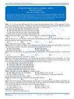
Figure 5A.1  The partial molar volumes of water and ethanol

at 25 °C. Note the different scales (water on the left, ethanol on
the right).

V(b)

Volume, V

Imagine a huge volume of pure water at 25 °C. When a further
1 mol H2O is added, the volume increases by 18 cm3 and we
can report that 18 cm3 mol−1 is the molar volume of pure water.
However, when we add 1 mol H2O to a huge volume of pure
ethanol, the volume increases by only 14 cm3. The reason for
the different increase in volume is that the volume occupied by
a given number of water molecules depends on the identity of
the molecules that surround them. In the latter case there is so
much ethanol present that each H2O molecule is surrounded by
ethanol molecules. The network of hydrogen bonds that normally hold H2O molecules at certain distances from each other
in pure water does not form. The packing of the molecules in
the mixture results in the H2O molecules increasing the volume
by only 14 cm3. The quantity 14 cm3 mol−1 is the partial molar
volume of water in pure ethanol. In general, the partial molar
volume of a substance A in a mixture is the change in volume
per mole of A added to a large volume of the mixture.
The partial molar volumes of the components of a mixture
vary with composition because the environment of each type of
molecule changes as the composition changes from pure A to
pure B. It is this changing molecular environment, and the consequential modification of the forces acting between molecules,
that results in the variation of the thermodynamic properties
of a mixture as its composition is changed. The partial molar
volumes of water and ethanol across the full composition range

at 25 °C are shown in Fig. 5A.1.
The partial molar volume, VJ , of a substance J at some general composition is defined formally as follows:

V(a)

a

b
Amount of A, nA

Figure 5A.2  The partial molar volume of a substance is the
slope of the variation of the total volume of the sample plotted
against the composition. In general, partial molar quantities
vary with the composition, as shown by the different slopes at
the compositions a and b. Note that the partial molar volume
at b is negative: the overall volume of the sample decreases as
A is added.

the slope of the plot of the total volume as the amount of J is
changed, the pressure, temperature, and amount of the other
components being constant (Fig. 5A.2). Its value depends on
the composition, as we saw for water and ethanol.
A note on good practice  The IUPAC recommendation is to
denote a partial molar quantity by X , but only when there is
the possibility of confusion with the quantity X. For instance,
to avoid confusion, the partial molar volume of NaCl in water
could be written V (NaCl, aq) to distinguish it from the total
volume of the solution, V.

The definition in eqn 5A.1 implies that when the composition of the mixture is changed by the addition of dnA of A and

dnB of B, then the total volume of the mixture changes by
 ∂V 
 ∂V 
dV = 
dnA + 
dnB

∂
n
 A  p,T ,n
 ∂nB  p,T ,n
B

(5A.2)

A

= VA dnA + VBdnB



Provided the relative composition is held constant as the
amounts of A and B are increased, the partial molar volumes
are both constant. In that case we can obtain the final volume
by integration, treating VA and VB as constants:
V=

∫

nA

0

VA dnA +

= VA nA + VBnB

∫

nB

0

VB dnB = VA

∫

nA

0

dnA + VB

∫

nB

0

dnB

(5A.3)



Although we have envisaged the two integrations as being
linked (in order to preserve constant relative composition),
because V is a state function the final result in eqn 5A.3 is valid
however the solution is in fact prepared.


182  5  Simple mixtures
Partial molar volumes can be measured in several ways. One
method is to measure the dependence of the volume on the
composition and to fit the observed volume to a function of the
amount of the substance. Once the function has been found,
its slope can be determined at any composition of interest by
differentiation.
Example 5A.1  Determining a partial molar volume

A polynomial fit to measurements of the total volume of a water/
ethanol mixture at 25 °C that contains 1.000 kg of water is
v =1002.93 + 54.6664 x − 0.363 94 x 2 + 0.028256 x 3
where v = V/cm 3 , x = n E /mol, and n E is the amount of
CH3CH2OH present. Determine the partial molar volume of
ethanol.
Method  Apply the definition in eqn 5A.1 taking care to con-

vert the derivative with respect to n to a derivative with respect
to x and keeping the units intact.

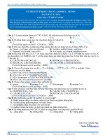
Answer  The partial molar volume of ethanol, VE , is

(
(

) 
) 

 ∂ V /cm3
 ∂V 
=
VE = 

 ∂nE  p,T ,n  ∂ nE/mol
W

p ,T ,nW

cm3
mol

Self-test 5A.1  At 25 °C, the density of a 50 per cent by mass
ethanol/water solution is 0.914 g cm−3. Given that the partial
molar volume of water in the solution is 17.4 cm3 mol−1, what is
the partial molar volume of the ethanol?
Answer: 56.4 cm3 mol−1; 54.6 cm3 mol−1 by the formula above

Molar volumes are always positive, but partial molar quantities need not be. For example, the limiting partial molar volume of MgSO4 in water (its partial molar volume in the limit
of zero concentration) is −1.4 cm3 mol−1, which means that the
addition of 1 mol MgSO4 to a large volume of water results in a

decrease in volume of 1.4 cm3. The mixture contracts because
the salt breaks up the open structure of water as the Mg2+ and
SO2−
4 ions become hydrated, and it collapses slightly.

(b)  Partial molar Gibbs energies
The concept of a partial molar quantity can be extended to
any extensive state function. For a substance in a mixture,
the chemical potential is defined as the partial molar Gibbs
energy:
 ∂G 
µJ = 
 ∂nJ  p ,T ,n′

 ∂v 
= 
cm3 mol −1
 ∂x  p,T ,n
W

Then, because

Chemical potential  (5A.4)

That is, the chemical potential is the slope of a plot of Gibbs
energy against the amount of the component J, with the pressure and temperature (and the amounts of the other substances) held constant (Fig. 5A.4). For a pure substance we can
write G = nJGJ,m, and from eqn 5A.4 obtain µJ = GJ,m: in this case,
the chemical potential is simply the molar Gibbs energy of the
substance, as is used in Topic 4B.

dv
= 54.6664 − 2(0.363 94)x + 3(0.028 256)x 2
dx
we can conclude that
VE /(cm3mol −1 ) = 54.6664 − 0.727 88 x + 0.084 768 x 2

Definition 





56

µ(b)
Gibbs energy, G

Partial molar volume, VE/(cm3 mol–1)

Figure 5A.3 shows a graph of this function.

55

µ(a)

54

a
53
0

b

Amount of A, nA
5
x = nE/mol

Figure 5A.3  The partial molar volume of ethanol, as
expressed by the polynomial in Example 5A.1.

10

Figure 5A.4  The chemical potential of a substance is the
slope of the total Gibbs energy of a mixture with respect to
the amount of substance of interest. In general, the chemical
potential varies with composition, as shown for the two values
at a and b. In this case, both chemical potentials are positive.


5A  The thermodynamic description of mixtures  
By the same argument that led to eqn 5A.2, it follows that the
total Gibbs energy of a binary mixture is
G = nA μA + nB μB

(5A.9)

and hence that

(5A.5)

where µA and µB are the chemical potentials at the composition
of the mixture. That is, the chemical potential of a substance
in a mixture is the contribution of that substance to the total
Gibbs energy of the mixture. Because the chemical potentials
depend on composition (and the pressure and temperature),
the Gibbs energy of a mixture may change when these variables
change, and for a system of components A, B, etc., the equation
dG = Vdp − SdT becomes
dG = Vdp − SdT + μA dnA + μB dnB +

Fundamental equation of chemical thermodynamics  (5A.6)

This expression is the fundamental equation of chemical thermodynamics. Its implications and consequences are explored
and developed in this and the next two chapters.
At constant pressure and temperature, eqn 5A.6 simplifies to
dG = μA dnA + μB dnB +

(5A.7)

We saw in Topic 3C that under the same conditions
dG = dwadd,max. Therefore, at constant temperature and pressure,
dwadd , max = μA dnA + μB dnB +

dU = μA dnA + μB dnB +

183



(5A.8)

That is, additional (non-expansion) work can arise from the
changing composition of a system. For instance, in an electrochemical cell, the chemical reaction is arranged to take place
in two distinct sites (at the two electrodes). The electrical work
the cell performs can be traced to its changing composition as
products are formed from reactants.

(c)  The wider significance of the chemical

potential

The chemical potential does more than show how G varies
with composition. Because G = U + pV − TS, and therefore
U = − pV + TS + G, we can write a general infinitesimal change in
U for a system of variable composition as
dU = − pdV − Vdp + SdT + TdS + dG
= − pdV − Vdp + SdT + TdS +
(Vdp − SdT + μA dnA + μB dnB +)
= − pdV + TdS + μA dnA + μB dnB +
This expression is the generalization of eqn 3D.1 (that
dU = TdS − pdV) to systems in which the composition may
change. It follows that at constant volume and entropy,

 ∂U 
µJ = 
 ∂nJ  S ,V ,n′

(5A.10)

Therefore, not only does the chemical potential show how G
changes when the composition changes, it also shows how the
internal energy changes too (but under a different set of conditions). In the same way it is possible to deduce that
 ∂H 
(a) µJ = 
 ∂nJ  S , p ,n′

 ∂A 
(b) µJ = 
 ∂nJ  T ,V ,n′

(5A.11)



Thus we see that the µJ shows how all the extensive thermodynamic properties U, H, A, and G depend on the composition. This is why the chemical potential is so central to
chemistry.

(d)  The Gibbs–Duhem equation
Because the total Gibbs energy of a binary mixture is given by
eqn 5A.5 and the chemical potentials depend on the composition, when the compositions are changed infinitesimally we
might expect G of a binary system to change by
dG = μA dnA + μB dnB + nA dμA + nB dμB
However, we have seen that at constant pressure and temperature a change in Gibbs energy is given by eqn 5A.7. Because G
is a state function, these two equations must be equal, which
implies that at constant temperature and pressure
nA dμA + nB dμB =0

(5A.12a)

This equation is a special case of the Gibbs–Duhem equation:

∑ n dμ = 0
J

J

Gibbs–Duhem equation  (5A.12b)

J



The significance of the Gibbs–Duhem equation is that the
chemical potential of one component of a mixture cannot
change independently of the chemical potentials of the other
components. In a binary mixture, if one partial molar quantity
increases, then the other must decrease, with the two changes
related by

dμ B = −

nA
dμ
nB A

(5A.13)

184  5  Simple mixtures
Brief illustration 5A.1  The Gibbs–Duhem equation

If the composition of a mixture is such that n A = 2n B , and
a small change in composition results in μ A changing by
δμ A = +1 J mol−1, μ B will change by
δμB = −2 × (1Jmol −1 ) = − 2 Jmol −1



Self-test 5A.2  Suppose that n A = 0.3n B and a small change in

composition results in μ A changing by δμ A = –10 J mol−1, by
how much will μ B change?
Answer: +3 J mol−1

vA = vA* − 9.108

∫

b/b <

0

nB −1/2
x dx
nA

However, the ratio of amounts of A (H 2O) and B (K 2SO 4) is
related to the molality of B, b = n B/(1 kg water) and n A = (1 kg

water)/MA where MA is the molar mass of water, by
nB
nB
nM
=
= B A = bM A = xb < M A
nA (1kg )/M A
1kg
and hence
vA = v *A − 9.108 M Ab <

The experimental values of the partial molar volume of
K 2SO4(aq) at 298 K are found to fit the expression
vB = 32.280 +18.216 x

Method  Let A denote H 2O, the solvent, and B denote K 2SO4,
the solute. The Gibbs–Duhem equation for the partial molar
volumes of two components is n AdVA + nBdVB = 0. This relation
implies that dvA = − (n B/n A)dvB, and therefore that vA can be
found by integration:

∫

vB

0

x1/2dx

It t hen fol lows, by substituting t he data (including

MA = 1.802 × 10−2 kg mol−1, the molar mass of water), that
VA / (cm3mol −1 ) =18.079 − 0.1094(b / b < )3/2
The partial molar volumes are plotted in Fig. 5A.5.
40

18.079

38

18.078

36

K2SO4

Water

18.076

34

1/2

where vB = VK2SO4 /(cm3 mol −1 ) and x is the numerical value of
the molality of K 2SO4 (x = b/b < ; see the remark in the introduction to this chapter). Use the Gibbs–Duhem equation to derive
an equation for the molar volume of water in the solution. The
molar volume of pure water at 298 K is 18.079 cm3 mol−1.

vA = vA* −

0

V(H2O)/
(cm3 mol–1)

Example 5A.2  Using the Gibbs–Duhem equation

b/b <

2
= vA* − (9.108 M Ab < )(b / b < )3/2
3


V(K2SO4)/(cm3 mol–1)

The same line of reasoning applies to all partial molar quantities. We can see in Fig. 5A.1, for example, that where the partial molar volume of water increases, that of ethanol decreases.
Moreover, as eqn 5A.13 shows, and as we can see from Fig 5A.1,
a small change in the partial molar volume of A corresponds to
a large change in the partial molar volume of B if nA/nB is large,
but the opposite is true when this ratio is small. In practice, the
Gibbs–Duhem equation is used to determine the partial molar
volume of one component of a binary mixture from measurements of the partial molar volume of the second component.

∫

nB
dv
nA B

where vA* =VA /(cm3 mol −1 ) is the numerical value of the molar
volume of pure A. The first step is to change the variable vB
to x = b/b < and then to integrate the right-hand side between
x = 0 (pure B) and the molality of interest.
Answer  It follows from the information in the question that,

with B = K 2SO4, dvB/dx = 9.108x−1/2. Therefore, the integration
required is

32
0

0.05

18.075
0.1

b/(mol kg–1)

Figure 5A.5  The partial molar volumes of the components
of an aqueous solution of potassium sulfate.
Self-test 5A.3  Repeat the calculation for a salt B for which VB/
(cm3 mol−1) = 6.218 + 5.146b − 7.147b2.
Answer: VA/(cm3 mol−1) = 18.079 − 0.0464b2 + 0.0859b3

5A.2  The

thermodynamics of mixing

The dependence of the Gibbs energy of a mixture on its composition is given by eqn 5A.5, and we know that at constant

temperature and pressure systems tend towards lower Gibbs
energy. This is the link we need in order to apply thermodynamics to the discussion of spontaneous changes of composition, as in the mixing of two substances. One simple example
of a spontaneous mixing process is that of two gases introduced
into the same container. The mixing is spontaneous, so it must


5A  The thermodynamic description of mixtures  
correspond to a decrease in G. We shall now see how to express
this idea quantitatively.

(a)  The Gibbs energy of mixing of perfect

gases

Let the amounts of two perfect gases in the two containers be
nA and nB; both are at a temperature T and a pressure p (Fig.
5A.6). At this stage, the chemical potentials of the two gases
have their ‘pure’ values, which are obtained by applying the defin­
ition μ = Gm to eqn 3D.15 (Gm(p) = Gm< + RT ln(p/p<)):
p
μ = μ < + RT ln <
p

Variation of chemical potential with pressure   (5A.14a)

where μ< is the standard chemical potential, the chemical
potential of the pure gas at 1 bar. It will be much simpler notationally if we agree to let p denote the pressure relative to p<;
that is, to replace p/p< by p, for then we can write
μ = μ < + RT ln p

∆ mixG = nRT (x A ln x A + x B ln x B )
Perfect gases 

Gi = nA μA + nB μB = nA ( μA< + RT ln p) + nB ( μB< + RT ln p)

(5A.15a)

After mixing, the partial pressures of the gases are pA and pB,
with pA+pB = p. The total Gibbs energy changes to
Gf = nA ( μA< + RT ln pA ) + nB ( μB< + RT ln pB )

(5A.15b)



(5A.15c)



Gibbs energy of mixing   (5A.16)

Because mole fractions are never greater than 1, the logarithms
in this equation are negative, and ΔmixG < 0 (Fig. 5A.7). The
conclusion that ΔmixG is negative for all compositions confirms that perfect gases mix spontaneously in all proportions.
However, the equation extends common sense by allowing us
to discuss the process quantitatively.
0

–0.2

(5A.14b)

To use the equations, we have to remember to replace p by p/p<
again. In practice, that simply means using the numerical value
of p in bars. The Gibbs energy of the total system is then given
by eqn 5A.5 as

pA
p
+ nB RT ln B
p
p

At this point we may replace nJ by xJn, where n is the total
amount of A and B, and use the relation between partial pressure and mole fraction (Topic 1A, pJ = xJp) to write pJ/p = xJ for
each component, which gives

ΔmixG/nRT

Perfect gas 

∆ mixG = nA RT ln

185

–0.4

–0.6

–0.8

0

0.5
Mole fraction of A, xA

1

Figure 5A.7  The Gibbs energy of mixing of two perfect
gases and (as discussed later) of two liquids that form an
ideal solution. The Gibbs energy of mixing is negative for
all compositions and temperatures, so perfect gases mix
spontaneously in all proportions.

The difference Gf − Gi, the Gibbs energy of mixing, ΔmixG, is
therefore
Example 5A.3  Calculating a Gibbs energy of mixing
nA, T, p

nB, T, p

A container is divided into two equal compartments (Fig.
5A.8). One contains 3.0 mol H2(g) at 25 °C; the other contains
1.0 mol N2(g) at 25 °C. Calculate the Gibbs energy of mixing
when the partition is removed. Assume perfect behaviour.
Method  Equation 5A.16 cannot be used directly because the two

T, pA, pB with pA + pB = p

Figure 5A.6  The arrangement for calculating the
thermodynamic functions of mixing of two perfect gases.

gases are initially at different pressures. We proceed by calculating the initial Gibbs energy from the chemical potentials. To do
so, we need the pressure of each gas. Write the pressure of nitrogen as p; then the pressure of hydrogen as a multiple of p can be
found from the gas laws. Next, calculate the Gibbs energy for the
system when the partition is removed. The volume occupied by
each gas doubles, so its initial partial pressure is halved.


186  5  Simple mixtures
(b)  Other thermodynamic mixing functions
3.0 mol H2

In Topic 3D it is shown that (∂G/∂T)p,n = –S. It follows immediately from eqn 5A.16 that, for a mixture of perfect gases initially
at the same pressure, the entropy of mixing, ΔmixS, is

1.0 mol N2

3p

p

3.0 mol H2
2p
p(H2) = 3/2p

 ∂∆ G 
∆ mix S = −  mix 
 ∂ T  p ,n

A ,nB

1.0 mol N2

Perfect gases 

p(N2) = 1/2p

0.8

0.6

of hydrogen is 3p; therefore, the initial Gibbs energy is
Gi = (3.0 mol ){μ < (H2 ) + RT ln 3 p} +
(1.0 mol){μ < (N2 ) + RT ln p}



Gf = (3.0 mol ){μ < (H2 ) + RT ln 23 p} +

p}

The Gibbs energy of mixing is the difference of these two
quantities:
1
p
p
+ (1.0 mol)RT ln 2
3p
p
= −(3.0 mol)RT ln 2 − (1.0 mol)RT ln 2

= −(4.0 mol )RT ln 2 = −6.9 kJ

∆ mixG = (3.0 mol)RT ln

0.4

0.2

When the partition is removed and each gas occupies twice
the original volume, the partial pressure of nitrogen falls to
1
3
p
2 and that of hydrogen falls to 2 p. Therefore, the Gibbs
energy changes to
1
2

ΔmixS/nR

Answer  Given that the pressure of nitrogen is p, the pressure

(1.0 mol){μ (N2 ) + RT ln



Entropy of mixing   (5A.17)

Because ln x < 0, it follows that ΔmixS > 0 for all compositions
(Fig. 5A.9).

Figure 5A.8  The initial and final states considered in
the calculation of the Gibbs energy of mixing of gases at
different initial pressures.

<

= −nR ( x A ln x A + x B ln x B )

3
2

0

0

0.5
Mole fraction of A, xA

1

Figure 5A.9  The entropy of mixing of two perfect gases and
(as discussed later) of two liquids that form an ideal solution.
The entropy increases for all compositions and temperatures,
so perfect gases mix spontaneously in all proportions.
Because there is no transfer of heat to the surroundings
when perfect gases mix, the entropy of the surroundings is
unchanged. Hence, the graph also shows the total entropy of
the system plus the surroundings when perfect gases mix.

In this example, the value of ΔmixG is the sum of two contributions: the mixing itself, and the changes in pressure of the two
gases to their final total pressure, 2p. When 3.0 mol H2 mixes
with 1.0 mol N2 at the same pressure, with the volumes of the
vessels adjusted accordingly, the change of Gibbs energy is
–5.6 kJ. However, do not be misled into interpreting this negative change in Gibbs energy as a sign of spontaneity: in this
case, the pressure changes, and ΔG < 0 is a signpost of spontaneous change only at constant temperature and pressure.
Self-test 5A.4  Suppose that 2.0 mol H 2 at 2.0 atm and 25 °C

and 4.0 mol N2 at 3.0 atm and 25 °C are mixed by removing the
partition between them. Calculate ΔmixG.

Answer: –9.7 kJ

Brief illustration 5A.2  The entropy of mixing

For equal amounts of perfect gas molecules that are mixed at
the same pressure we set x A = x B = 12 and obtain
∆ mix S = − nR{ 12 ln

1
2

+ 12 ln 12 } = nR ln 2

with n the total amount of gas molecules. For 1 mol of each
species, so n = 2 mol,
∆ mix S = (2 mol ) × R ln 2 = + 11.5Jmol −1
An increase in entropy is what we expect when one gas disperses into the other and the disorder increases.

5A  The thermodynamic description of mixtures  

187

Self-test 5A.5  Calculate the change in entropy for the arrangement in Example 5A.3.
Answer: +23 J mol−1
A(g) + B(g)

µA(g, p)

=

We can calculate the isothermal, isobaric (constant pressure)
enthalpy of mixing, ΔmixH, the enthalpy change accompanying mixing, of two perfect gases from ΔG = ΔH − TΔS. It follows
from eqns 5A.16 and 5A.17 that
Perfect gases 

Enthalpy of mixing   (5A.18)

The enthalpy of mixing is zero, as we should expect for a system
in which there are no interactions between the molecules forming the gaseous mixture. It follows that the whole of the driving force for mixing comes from the increase in entropy of the
system because the entropy of the surroundings is unchanged.

5A.3  The

chemical potentials
of liquids

(a)  Ideal solutions
We shall denote quantities relating to pure substances by a
superscript *, so the chemical potential of pure A is written
μA* and as μA* (l) when we need to emphasize that A is a liquid.
Because the vapour pressure of the pure liquid is pA* it follows
from eqn 5A.14 that the chemical potential of A in the vapour
(treated as a perfect gas) is μA< = +RT ln pA (with pA to be interpreted as the relative pressure, pA/p<). These two chemical
potentials are equal at equilibrium (Fig. 5A.10), so we can write
(5A.19a)

If another substance, a solute, is also present in the liquid, the
chemical potential of A in the liquid is changed to μA and its
vapour pressure is changed to pA. The vapour and solvent are
still in equilibrium, so we can write
μA = μA< + RT ln pA

Figure 5A.10  At equilibrium, the chemical potential of
the gaseous form of a substance A is equal to the chemical
potential of its condensed phase. The equality is preserved if
a solute is also present. Because the chemical potential of A in
the vapour depends on its partial vapour pressure, it follows
that the chemical potential of liquid A can be related to its
partial vapour pressure.

μA = μA* − RT ln pA* + RT ln pA = μA* + RT ln

To discuss the equilibrium properties of liquid mixtures we
need to know how the Gibbs energy of a liquid varies with
composition. To calculate its value, we use the fact that, as
established in Topic 4A, at equilibrium the chemical potential

of a substance present as a vapour must be equal to its chemical
potential in the liquid.

μA* = μA< + RT ln pA*

A(l) + B(l)

pA
pA*

(5A.20)

In the final step we draw on additional experimental information about the relation between the ratio of vapour pressures
and the composition of the liquid. In a series of experiments on
mixtures of closely related liquids (such as benzene and methyl­
benzene), the French chemist François Raoult found that the
ratio of the partial vapour pressure of each component to its
vapour pressure as a pure liquid, pA /pA* , is approximately equal
to the mole fraction of A in the liquid mixture. That is, he established what we now call Raoult’s law:
pA = x A pA*

Ideal solution 

Raoult’s law   (5A.21)

This law is illustrated in Fig. 5A.11. Some mixtures obey
Raoult’s law very well, especially when the components are

pB*

Pressure

∆ mix H = 0

µA(l)

Total
pressure
Partial
pressure
of B
Partial
pressure
of A

pA*

(5A.19b)

Next, we combine these two equations to eliminate the standard chemical potential of the gas. To do so, we write eqn 5A.19a
as μA< = μA* − RT ln pA* and substitute this expression into eqn
5A.19b to obtain

Mole fraction of A, xA

Figure 5A.11  The total vapour pressure and the two partial
vapour pressures of an ideal binary mixture are proportional to
the mole fractions of the components.

188  5  Simple mixtures
80

500

Total
Benzene

Pressure, p/Torr

Pressure, p/Torr

60

400

Total
40

20

0
Mole fraction of methylbenzene, x(C6H5CH3)

1

Figure 5A.12  Two similar liquids, in this case benzene and
methylbenzene (toluene), behave almost ideally, and the
variation of their vapour pressures with composition resembles
that for an ideal solution.

structurally similar (Fig. 5A.12). Mixtures that obey the law
throughout the composition range from pure A to pure B are
called ideal solutions.
Brief illustration 5A.3  Raoult’s law

The vapour pressure of benzene at 20 °C is 75 Torr and that of
methylbenzene is 21 Torr at the same temperature. In an equimolar mixture, x benzene = x methylbenzene = 12 so the vapour pressure of each one in the mixture is
pbenzene = 12 × 75 Torr = 38Torr

pmethylbenzene = 12 × 21 Torr =11Torr

The total vapour pressure of the mixture is 49 Torr. Given
the two partial vapour pressures, it follows from the definition of partial pressure (Topic 1A) that the mole fractions
in the vapour are x vap,benzene = (38 Torr)/(49 Torr) = 0.78 and
x vap,methylbenzene = (11 Torr)/(49 Torr) = 0.22. The vapour is richer
in the more volatile component (benzene).
Self-test 5A.6  At 90 °C the vapour pressure of 1,2-dimethy­l­

benzene is 20 kPa and that of 1,3-dimethylbenzene is 18 kPa.
What is the composition of the vapour when the liquid mixture has the composition x12 = 0.33 and x13 = 0.67?
Answer: x vap,12 = 0.35, x vap,13 = 0.65

For an ideal solution, it follows from eqns 5A.19a and 5A.21
that
μA = μA* + RT ln x A

Carbon disulfide

200

Acetone
100

Methylbenzene

0

300

Ideal solution 

Chemical potential   (5A.22)

This important equation can be used as the definition of an ideal
solution (so that it implies Raoult’s law rather than stemming

0
0

Mole fraction of carbon disulfide, x(CS2)

1

Figure 5A.13  Strong deviations from ideality are shown by
dissimilar liquids, in this case carbon disulfide and acetone
(propanone).

from it). It is in fact a better definition than eqn 5A.21 because
it does not assume that the vapour is a perfect gas.

The molecular origin of Raoult’s law is the effect of the
solute on the entropy of the solution. In the pure solvent,
the molecules have a certain disorder and a corresponding
entropy; the vapour pressure then represents the tendency
of the system and its surroundings to reach a higher entropy.
When a solute is present, the solution has a greater disorder
than the pure solvent because we cannot be sure that a molecule chosen at random will be a solvent molecule. Because the
entropy of the solution is higher than that of the pure solvent,
the solution has a lower tendency to acquire an even higher
entropy by the solvent vaporizing. In other words, the vapour
pressure of the solvent in the solution is lower than that of the
pure solvent.
Some solutions depart significantly from Raoult’s law (Fig.
5A.13). Nevertheless, even in these cases the law is obeyed
increasingly closely for the component in excess (the solvent)
as it approaches purity. The law is another example of a limiting
law (in this case, achieving reliability as xA → 1) and is a good
approximation for the properties of the solvent if the solution
is dilute.

(b)  Ideal–dilute solutions
In ideal solutions the solute, as well as the solvent, obeys Raoult’s
law. However, the English chemist William Henry found experimentally that, for real solutions at low concentrations, although
the vapour pressure of the solute is proportional to its mole fraction, the constant of proportionality is not the vapour pressure
of the pure substance (Fig. 5A.14). Henry’s law is:
pB = x B K B

Ideal–dilute solution 

Henry’s law   (5A.23)

In this expression, xB is the mole fraction of the solute and
KB is an empirical constant (with the dimensions of pressure)


5A  The thermodynamic description of mixtures  

Example 5A.4  Investigating the validity of Raoult’s and

KB

Henry’s laws
The vapour pressures of each component in a mixture of propanone (acetone, A) and trichloromethane (chloroform, C)
were measured at 35 °C with the following results:

p*
B

Ideal solution
(Raoult)
0

Mole fraction of B, xB

1

Figure 5A.14  When a component (the solvent) is nearly pure,
it has a vapour pressure that is proportional to mole fraction
with a slope pB* (Raoult’s law). When it is the minor component
(the solute) its vapour pressure is still proportional to the mole

fraction, but the constant of proportionality is now KB (Henry’s
law).

chosen so that the plot of the vapour pressure of B against its
mole ­fraction is tangent to the experimental curve at xB = 0.
Henry’s law is therefore also a limiting law, achieving reliability
as xB → 0.
Mixtures for which the solute B obeys Henry’s law and
the solvent A obeys Raoult’s law are called ideal–dilute solutions. The difference in behaviour of the solute and solvent
at low concentrations (as expressed by Henry’s and Raoult’s
laws, respectively) arises from the fact that in a dilute solution
the solvent molecules are in an environment very much like
the one they have in the pure liquid (Fig. 5A.15). In contrast,
the solute molecules are surrounded by solvent molecules,
which is entirely different from their environment when pure.
Thus, the solvent behaves like a slightly modified pure liquid,
but the ­solute behaves entirely differently from its pure state
unless the ­solvent and solute molecules happen to be very similar. In the latter case, the solute also obeys Raoult’s law.

xC
0
0.20
0.40
0.60
0.80
1
pC/kPa
0
4.7
11

18.9
26.7
36.4
pA/kPa
46.3
33.3
23.3
12.3
4.9
0
Confirm that the mixture conforms to Raoult’s law for the
component in large excess and to Henry’s law for the minor
component. Find the Henry’s law constants.
Method  Both Raoult’s and Henry’s laws are statements about

the form of the graph of partial vapour pressure against mole
fraction. Therefore, plot the partial vapour pressures against
mole fraction. Raoult’s law is tested by comparing the data
with the straight line p J = x J p *J for each component in the
region in which it is in excess (and acting as the solvent).
Henry’s law is tested by finding a straight line p J = x J K *J that
is tangent to each partial vapour pressure at low x, where the
component can be treated as the solute.

Answer  The data are plotted in Fig. 5A.16 together with the
Raoult’s law lines. Henry’s law requires K A = 16.9 kPa for propanone and KC = 20.4 kPa for trichloromethane. Notice how
the system deviates from both Raoult’s and Henry’s laws even
for quite small departures from x = 1 and x = 0, respectively.
We deal with these deviations in Topic 5E.
50

p*(acetone)
40
Pressure, p/kPa

Pressure, p

Ideal–dilute
solution
(Henry)
Real
solution

189

p*(chloroform)
30
20

Raoult’s law
K(acetone)
K(chloroform)

10

Henry’s law
0

0

1

Mole fraction of chloroform, x(CHCl3)

Figure 5A.16  The experimental partial vapour pressures
of a mixture of chloroform (trichloromethane) and acetone
(propanone) based on the data in Example 5A.3. The values
of K are obtained by extrapolating the dilute solution
vapour pressures, as explained in the Example.
Self-test 5A.7  The vapour pressure of chloromethane at various

mole fractions in a mixture at 25 °C was found to be as follows:

Figure 5A.15  In a dilute solution, the solvent molecules
(the blue spheres) are in an environment that differs only
slightly from that of the pure solvent. The solute particles
(the purple spheres), however, are in an environment totally
unlike that of the pure solute.

x
0.005
0.009
p/kPa
27.3
48.4
Estimate Henry’s law constant.

0.019
101

0.024

126
Answer: 5 MPa


190  5  Simple mixtures
For practical applications, Henry’s law is expressed in terms
of the molality, b, of the solute, pB = bBKB. Some Henry’s law
data for this convention are listed in Table 5A.1. As well as providing a link between the mole fraction of solute and its partial
pressure, the data in the table may also be used to calculate gas
solubilities. A knowledge of Henry’s law constants for gases in
blood and fats is important for the discussion of respiration,
especially when the partial pressure of oxygen is abnormal, as
in diving and mountaineering, and for the discussion of the
action of gaseous anaesthetics.
Table 5A.1*  Henry’s law constants for gases in water at 298 K,
K/(kPa kg mol−1)
K/(kPa kg mol−1)
CO2

3.01 × 103

H2

1.28 × 105

N2

1.56 × 105

O2

7.92 × 104

Brief illustration 5A.4  Henry’s law and gas solubility

To estimate the molar solubility of oxygen in water at 25 °C
and a partial pressure of 21 kPa, its partial pressure in the
atmosphere at sea level, we write
bO2 =

pO2
21 kPa
=
= 2.9 ×10−4 mol kg −1
K O2 7.9 ×104 kPa kg mol −1

The mola lit y of t he saturated solut ion is t herefore
0.29 mmol kg−1. To convert this quantity to a molar concentration, we assume that the mass density of this dilute solution is
essentially that of pure water at 25 °C, or ρ = 0.997 kg dm−3. It
follows that the molar concentration of oxygen is
[O2 ] = bO2 ρ = (2.9 ×10−4 mol kg −1 ) × (0.997 kg dm −3 )
= 0.29 mmol dm −3
Self-test 5A.8  Calculate the molar solubility of nitrogen in

water exposed to air at 25 °C; partial pressures were calculated
in Example 1A.3 of Topic 1A.

Answer: 0.51 mmol dm−3

* More values are given in the Resource section.

Checklist of concepts
☐1.The molar concentration of a solute is the amount of
solute divided by the volume of the solution.
☐2.The molality of a solute is the amount of solute divided
by the mass of solvent.
☐3.The partial molar volume of a substance is the contribution to the volume that a substance makes when it is
part of a mixture.
☐4.The chemical potential is the partial molar Gibbs
energy and enables us to express the dependence of the
Gibbs energy on the composition of a mixture.
☐5.The chemical potential also shows how, under a variety
of different conditions, the thermodynamic functions
vary with composition.
☐6.The Gibbs–Duhem equation shows how the changes in
chemical potential of the components of a mixture are
related.

☐7.The Gibbs energy of mixing is calculated by forming
the difference of the Gibbs energies before and after
mixing: the quantity is negative for perfect gases at the
same pressure.
☐8.The entropy of mixing of perfect gases initially at the
same pressure is positive and the enthalpy of mixing is
zero.
☐9.Raoult’s law provides a relation between the vapour
pressure of a substance and its mole fraction in a mixture; it is the basis of the definition of an ideal solution.
☐10. Henry’s law provides a relation between the vapour
pressure of a solute and its mole fraction in a mixture; it
is the basis of the definition of an ideal–dilute solution.

Checklist of equations
Property

Equation

Comment

Equation number

Partial molar volume

VJ = (∂V/∂nJ)p,T,n′

Definition

5A.1

Chemical potential

µJ = (∂G/∂nJ)p,T,n′

Definition

5A.4

Total Gibbs energy

G = nAμA + nBμB

5A.5


5A  The thermodynamic description of mixtures  

Property

Equation

Comment

Fundamental equation of chemical
thermodynamics

dG = Vdp – SdT + μAdnA + μBdnB+…

5A.6

Gibbs–Duhem equation

∑JnJdμJ = 0

5A.12b

Chemical potential of a gas

μ = μ< + RT ln (p/p<)

Perfect gas

5A.14a

Gibbs energy of mixing

ΔmixG = nRT(xA ln xA + xB ln xB)

Perfect gases and ideal solutions

5A.16

Entropy of mixing

ΔmixS = –nR(xA ln xA + xB ln xB)

Perfect gases and ideal solutions

5A.17

Enthalpy of mixing

ΔmixH = 0

Perfect gases and ideal solutions

5A.18

Raoult’s law

pA = x A pA*

True for ideal solutions; limiting law as xA→1

5A.21

Chemical potential of component

μA = μA* + RT ln x A

Ideal solution

5A.22

Henry’s law

pB = xBKB

True for ideal–dilute solutions; limiting law as xB → 0

5A.23

191

Equation number


5B  The properties of solutions
Contents
5B.1 

Liquid mixtures

Ideal solutions
Brief illustration 5B.1: Ideal solutions
(b) Excess functions and regular solutions
Brief illustration 5B.2: Excess functions
Example 5B.1: Identifying the parameter
for a regular solution
(a)

5B.2 

Colligative properties
The common features of colligative properties
(b) The elevation of boiling point
Brief illustration 5B.3: Elevation of boiling point
(c) The depression of freezing point
Brief illustration 5B.4: Depression of freezing point
(d) Solubility
Brief illustration 5B.5: Ideal solubility
(e) Osmosis
Example 5B.2: Using osmometry to determine
the molar mass of a macromolecule
(a)

Checklist of concepts
Checklist of equations

192
192
193
193

194

First, we consider the simple case of mixtures of liquids that mix
to form an ideal solution. In this way, we identify the thermodynamic consequences of molecules of one species mingling
randomly with molecules of the second species. The calculation
provides a background for discussing the deviations from ideal
behaviour exhibited by real solutions. Then we consider the
effect of a solute on the properties of ideal and real solutions.

195
195
195
196
197
197
197
198
198
199
200
201
201

5B.1  Liquid

mixtures

Thermodynamics can provide insight into the properties of liquid mixtures, and a few simple ideas can bring the whole field
of study together. The development here is based on the relation derived in Topic 5A between the chemical potential of a
component (which here we call J for reasons that will become

clear) in an ideal mixture or solution, μJ, its value when pure,
μJ* , and its mole fraction in the mixture, xJ:
μJ = μJ* + RT ln x J

Ideal solution 

Chemical potential   (5B.1)

(a)  Ideal solutions
➤➤ Why do you need to know this material?
Mixtures and solutions play a central role in chemistry, and
it is important to understand how their compositions affect
their thermodynamic properties, such as their boiling and
freezing points. One very important property of a solution
is its osmotic pressure, which is used, among other things,
to determine the molar masses of macromolecules.

➤➤ What is the key idea?
The chemical potential of a substance in a mixture is the
same in each phase in which it occurs.

➤➤ What do you need to know already?
This Topic is based on the expression derived from Raoult’s
law (Topic 5A) in which chemical potential is related to
mole fraction. The derivations make use of the Gibbs–
Helmholtz equation (Topic 3D) and the effect of pressure
on chemical potential (Topic 3D). Some of the derivations
are the same as those used in the discussion of the mixing
of perfect gases (Topic 5A).

The Gibbs energy of mixing of two liquids to form an ideal
solution is calculated in exactly the same way as for two gases
(Topic 5A). The total Gibbs energy before liquids are mixed is
Gi = nA μA* + nB μB*

(5B.2a)

where the * denotes the pure liquid. When they are mixed, the
individual chemical potentials are given by eqn 5B.1 and the
total Gibbs energy is
Gf = nA (μ A* + RT ln x A ) + nB (μB* + RT ln x B )

(5B.2b)

Consequently, the Gibbs energy of mixing, the difference of
these two quantities, is
∆ mix G = nRT (x A ln x A + x B ln x B )



Gibbs energy
Ideal
solution of mixing

(5B.3)

where n = nA + nB. As for gases, it follows that the ideal entropy
of mixing of two liquids is
∆ mix S = −nR(x A ln x A + x B ln x B )

Entropy of
Ideal
solution mixing

(5B.4)


5B  The properties of solutions  
Because ΔmixH = ΔmixG + TΔmixS = 0, the ideal enthalpy of mixing is zero, ΔmixH = 0. The ideal volume of mixing, the change
in volume on mixing, is also zero because it follows from eqn
3D.8 ((∂G/∂p)T = V) that ΔmixV = (∂ΔmixG/∂p)T, but ΔmixG in eqn
5B.3 is independent of pressure, so the derivative with respect
to pressure is zero.
Equations 5B.3 and 5B.4 are the same as those for the mixing of two perfect gases and all the conclusions drawn there are
valid here: the driving force for mixing is the increasing entropy
of the system as the molecules mingle and the enthalpy of mixing is zero. It should be noted, however, that solution ideality
means something different from gas perfection. In a perfect gas
there are no forces acting between molecules. In ideal solutions
there are interactions, but the average energy of A–B interactions in the mixture is the same as the average energy of A–A
and B–B interactions in the pure liquids. The variation of the
Gibbs energy and entropy of mixing with composition is the
same as that for gases (Figs. 5A.7 and 5A.9); both graphs are
repeated here (as Figs. 5B.1 and 5B.2).
A note on good practice  It is on the basis of this distinc-

tion that the term ‘perfect gas’ is preferable to the more
0

ΔmixG/nRT

common ‘ideal gas’. In an ideal solution there are interactions, but they are effectively the same between the various
species. In a perfect gas, not only are the interactions the
same, but they are also zero. Few people, however, trouble
to make this valuable distinction.
Brief illustration 5B.1  Ideal solutions

Consider a mixture of benzene and methylbenzene, which
form an approximately ideal solution, and suppose 1.0 mol
C 6H6(l) is mixed with 2.0 mol C 6H5CH3(l). For the mixture,
x benzene = 0.33 and x methylbenzene = 0.67. The Gibbs energy and
entropy of mixing at 25 °C, when RT = 2.48 kJ mol−1, are
∆ mixG /n = (2.48 kJmol −1) × (0.33 ln 0.33 + 0.67 ln 0.67)
= −1.6 kJmol −1
∆ mix S /n = –(8.3145 J K −1 mol −1) × (0.33 ln 0.33 + 0.67 ln 0.67)
= +5.3JK –1 mol –1
The enthalpy of mixing is zero (presuming that the solution
is ideal).
Self-test 5B.1  Calculate the Gibbs energy and entropy of mixing when the proportions are reversed.
Answer: same: –1.6 kJ mol−1, + 5.3 J K−1 mol−1

–0.2

0.8

Real solutions are composed of particles for which A–A,
A–B, and B–B interactions are all different. Not only may
there be enthalpy and volume changes when liquids mix,
but there may also be an additional contribution to the

entropy arising from the way in which the molecules of one
type might cluster together instead of mingling freely with
the others. If the enthalpy change is large and positive or if
the entropy change is adverse (because of a reorganization
of the molecules that results in an orderly mixture), then
the Gibbs energy might be positive for mixing. In that case,
separation is spontaneous and the liquids may be immiscible. Alternatively, the liquids might be partially miscible,
which means that they are miscible only over a certain range
of compositions.

0.6

(b)  Excess functions and regular solutions

–0.4

–0.6

–0.8
0

0.5
Mole fraction of A, xA

1

Figure 5B.1  The Gibbs energy of mixing of two liquids that
form an ideal solution.

ΔmixS/nR

193

The thermodynamic properties of real solutions are expressed
in terms of the excess functions, XE, the difference between the
observed thermodynamic function of mixing and the function
for an ideal solution:

0.4

0.2

0

X E = ∆ mix X − ∆ mix X ideal
0

0.5
Mole fraction of A, xA

1

Figure 5B.2  The entropy of mixing of two liquids that form an
ideal solution.

Definition 

Excess function  (5B.5)

The excess entropy, SE, for example, is calculated using the

value of ΔmixSideal given by eqn 5B.4. The excess enthalpy and
volume are both equal to the observed enthalpy and volume of
mixing, because the ideal values are zero in each case.


194  5  Simple mixtures
H E = nξRTx A x B

Brief illustration 5B.2  Excess functions

Figure 5B.3 shows two examples of the composition dependence of molar excess functions. In Fig 5B.3a, the positive values of HE , which implies that Δmix H > 0, indicate that the A–B
interactions in the mixture are less attractive than the A–A
and B–B interactions in the pure liquids (which are benzene
and pure cyclohexane). The symmetrical shape of the curve
reflects the similar strengths of the A–A and B–B interactions.
Figure 5B.3b shows the composition dependence of the excess
volume, V E , of a mixture of tetrachloroethene and cyclopentane. At high mole fractions of cyclopentane, the solution contracts as tetrachloroethene is added because the ring
structure of cyclopentane results in inefficient packing of the
molecules but as tetrachloroethene is added, the molecules in
the mixture pack together more tightly. Similarly, at high mole
fractions of tetrachloroethene, the solution expands as cyclopentane is added because tetrachloroethene molecules are
nearly flat and pack efficiently in the pure liquid but become
disrupted as bulky ring cyclopentane is added.

∆ mix G = nRT (x A ln x A + x B ln x B + ξx A x B )

(5B.7)

Figure 5B.5 shows how ΔmixG varies with composition for
different values of ξ. The important feature is that for ξ > 2

the graph shows two minima separated by a maximum. The
implication of this observation is that, provided ξ > 2, then the
+0.5

400

2

0

1

–4

H E/nRT

H E/(J mol–1)

V E/(mm3 mol–1)

4

–8

(a)

where ξ (xi) is a dimensionless parameter that is a measure of
the energy of AB interactions relative to that of the AA and BB
interactions. (For HE expressed as a molar quantity, discard
the n.) The function given by eqn 5B.6 is plotted in Fig. 5B.4,

and we see it resembles the experimental curve in Fig. 5B.3a. If
ξ < 0, mixing is exothermic and the solute–solvent interactions
are more favourable than the solvent–solvent and solute–solute
interactions. If ξ > 0, then the mixing is endothermic. Because
the entropy of mixing has its ideal value for a regular solution,
the excess Gibbs energy is equal to the excess enthalpy, and the
Gibbs energy of mixing is

8

800

0

(5B.6)

0

0.5
x(C6H6)

1

–12

(b)

0

0.5

x(C2Cl4)

0

0

–1

1

Figure 5B.3  Experimental excess functions at 25 °C. (a) HE
for benzene/cyclohexane; this graph shows that the mixing
is endothermic (because ΔmixH = 0 for an ideal solution). (b)
The excess volume, V E , for tetrachloroethene/cyclopentane;
this graph shows that there is a contraction at low
tetrachloroethene mole fractions, but an expansion at high
mole fractions (because ΔmixV = 0 for an ideal mixture).
Self-test 5B.2  Would you expect the excess volume of mixing

–2
–0.5

+0.1

1

3

0

2.5
–0.1

ΔmixG/nRT

Deviations of the excess energies from zero indicate the
extent to which the solutions are non-ideal. In this connection a useful model system is the regular solution, a solution
for which HE  ≠ 0 but SE = 0. We can think of a regular solution
as one in which the two kinds of molecules are distributed
randomly (as in an ideal solution) but have different energies
of interactions with each other. To express this concept more
quantitatively we can suppose that the excess enthalpy depends
on composition as

0.5
xA

Figure 5B.4  The excess enthalpy according to a model in
which it is proportional to ξxA xB, for different values of the
parameter ξ.

of oranges and melons to be positive or negative?

Answer: Positive; close-packing disrupted

0

2

–0.2

1.5

–0.3

1

–0.4
–0.5

0

0.5
xA

1

Figure 5B.5  The Gibbs energy of mixing for different values of
the parameter ξ.


5B  The properties of solutions  
system will separate spontaneously into two phases with compositions corresponding to the two minima, for that separation
corresponds to a reduction in Gibbs energy. We develop this
point in Topic 5C.

properties

solution
Identify the value of the parameter ξ that would be appropriate to model a mixture of benzene and cyclohexane at 25 °C

and estimate the Gibbs energy of mixing to produce an equimolar mixture.
Method  Refer to Fig. 5B.3a and identify the value at the curve

maximum, and then relate it to eqn 5B.6 written as a molar
quantity (H E = ξRTx A x B). For the second part, assume that
the solution is regular and that the Gibbs energy of mixing is
given by eqn 5B.7.
Answer  The experimental value occurs close to x A = x B = 12 and

its value is close to 710 J mol−1. It follows that

HE
701J mol −1
=
= 1.13
−
1
RTx A x B (8.3145 J K mol −1) × (298 K) × 12 × 12



The total Gibbs energy of mixing to achieve the stated composition (provided the solution is regular) is therefore
∆ mixG / n = − RT ln 2 + 701Jmol −1
= − 1.72 kJmol −1 + 0.701kJmol −1 = − 1.022 kJmol −1
Self-test 5B.3  Fit the entire data set, as best as can be inferred

from the graph in Fig. 5B.3a, to an expression of the form in
eqn 5B.6 by a curve-fitting procedure.
Answer: The best fit of the form Ax(1 – x) to the data pairs

X
HE/(J mol−1)

0.1 0.2 0.3 0.4 0.5

0.6

0.7 0.8

pure solid solvent separates when the solution is frozen. The
latter assumption is quite drastic, although it is true of many
mixtures; it can be avoided at the expense of more algebra, but
that introduces no new principles.

(a)  The common features of colligative

Example 5B.1  Identifying the parameter for a regular

ξ=

195

0.9

150 350 550 680 700 690 600 500 280

All the colligative properties stem from the reduction of the
chemical potential of the liquid solvent as a result of the presence of solute. For an ideal solution (one that obeys Raoult’s
law, Topic 5A; pA = x A pA* ), the reduction is from μ A* for the pure
solvent to μ A = μ A* + RT ln x A when a solute is present (ln xA

is negative because xA < 1). There is no direct influence of the
solute on the chemical potential of the solvent vapour and the
solid solvent because the solute appears in neither the vapour
nor the solid. As can be seen from Fig. 5B.6, the reduction in
chemical potential of the solvent implies that the liquid–vapour
equilibrium occurs at a higher temperature (the boiling point is
raised) and the solid–liquid equilibrium occurs at a lower temperature (the freezing point is lowered).
The molecular origin of the lowering of the chemical potential is not the energy of interaction of the solute and solvent
particles, because the lowering occurs even in an ideal solution
(for which the enthalpy of mixing is zero). If it is not an enthalpy
effect, it must be an entropy effect. The vapour pressure of the
pure liquid reflects the tendency of the solution towards greater
entropy, which can be achieved if the liquid vaporizes to form
a gas. When a solute is present, there is an additional contribution to the entropy of the liquid, even in an ideal solution.
Because the entropy of the liquid is already higher than that of
the pure liquid, there is a weaker tendency to form the gas (Fig.
5B.7). The effect of the solute appears as a lowered vapour pressure, and hence a higher boiling point. Similarly, the enhanced
molecular randomness of the solution opposes the tendency
to freeze. Consequently, a lower temperature must be reached

5B.2  Colligative

properties

The properties we consider are the lowering of vapour pressure,
the elevation of boiling point, the depression of freezing point,
and the osmotic pressure arising from the presence of a solute.
In dilute solutions these properties depend only on the number
of solute particles present, not their identity. For this reason,
they are called colligative properties (denoting ‘depending on

the collection’). In this development, we denote the solvent by
A and the solute by B.
We assume throughout the following that the solute is not
volatile, so it does not contribute to the vapour. We also assume
that the solute does not dissolve in the solid solvent: that is, the

Chemical potential, µ

is A = 690 J mol−1
Pure
liquid
Solid

Vapour
Solution

Freezing
point
depression
Tf ’

Tf

Boiling
point
elevation
Tb

Tb’

Temperature, T

Figure 5B.6  The chemical potential of a solvent in the
presence of a solute. The lowering of the liquid’s chemical
potential has a greater effect on the freezing point than on the
boiling point because of the angles at which the lines intersect.


196  5  Simple mixtures
μ A* (g) = μ A* (l) + RT ln x A
pA*

pA

(The pressure of 1 atm is the same throughout, and will not be
written explicitly.) We show in the following Justification that
this equation implies that the presence of a solute at a mole
fraction xB causes an increase in normal boiling point from T*
to T* + ΔTb, where
∆Tb = Kx B

(a)

(5B.8)

K=

RT *2
∆ vap H

Ideal
solution

Elevation of
boiling point

(5B.9)

(b)

Figure 5B.7  The vapour pressure of a pure liquid represents
a balance between the increase in disorder arising from
vaporization and the decrease in disorder of the surroundings.
(a) Here the structure of the liquid is represented highly
schematically by the grid of squares. (b) When solute (the dark
squares) is present, the disorder of the condensed phase is
higher than that of the pure liquid, and there is a decreased
tendency to acquire the disorder characteristic of the vapour.

before equilibrium between solid and solution is achieved.
Hence, the freezing point is lowered.
The strategy for the quantitative discussion of the elevation of
boiling point and the depression of freezing point is to look for
the temperature at which, at 1 atm, one phase (the pure solvent
vapour or the pure solid solvent) has the same chemical potential
as the solvent in the solution. This is the new equilibrium temperature for the phase transition at 1 atm, and hence corresponds
to the new boiling point or the new freezing point of the solvent.

(b)  The elevation of boiling point
The heterogeneous equilibrium of interest when considering

boiling is between the solvent vapour and the solvent in solution at 1 atm (Fig. 5B.8). The equilibrium is established at a
temperature for which

Justification 5B.1  The elevation of the boiling point

of a solvent
Equation 5B.8 can be rearranged into
ln x A =

μ A* (g) − μ A* (l) ∆ vapG
=
RT
RT

where Δ vap G is the Gibbs energy of vaporization of the
pure  solvent (A). First, to find the relation between a
change in composition and the resulting change in boiling
temperature, we differentiate both sides with respect to temperature and use the Gibbs–Helmholtz equation (Topic 3D,
(∂(G/T)/∂T)p = −H/T2) to express the term on the right:
∆ vap H
d ln x A 1 d(∆ vapG /T )
=
=−
dT
R
dT
RT 2
Now multiply both sides by dT and integrate from x A = 1, corresponding to ln x A = 0 (and when T = T*, the boiling point of
pure A) to x A (when the boiling point is T):

∫

ln x A

0

d ln x A = −

µA*(g,p)

∫

T

T*

∆ vap H
dT
T2

The left-hand side integrates to ln x A , which is equal to
ln(1 – x B). The right-hand side can be integrated if we assume
that the enthalpy of vaporization is a constant over the small
range of temperatures involved and can be taken outside the
integral. Thus, we obtain
ln(1 − x B ) = −

A(g)

1

R

∆ vap H
R

∫

T

1

T* T

2

dT

and therefore

=
µA(l)

ln(1 − x B ) =

A(l) + B

Figure 5B.8  The heterogeneous equilibrium involved in the
calculation of the elevation of boiling point is between A in the
pure vapour and A in the mixture, A being the solvent and B a
non-volatile solute.

∆ vap H  1 1 
−
R  T T * 

We now suppose that the amount of solute present is so small
that x B ≪ 1, and use the expansion ln (1 − x) = − x − 12 x 2 + … ≈ − x
(Mathematical background 1) and hence obtain
xB =

∆ vap H  1 1 
−
R  T * T 


5B  The properties of solutions  

197

Finally, because T ≈ T*, it also follows that
1 1 T − T * T − T * ∆Tb
− =
≈
= 2
T * T TT *
T *2
T*

A(l) + B

=

with ΔTb = T – T*. The previous equation then rearranges into
eqn 5B.9.

Because eqn 5B.9 makes no reference to the identity of the
solute, only to its mole fraction, we conclude that the elevation of boiling point is a colligative property. The value of ΔT
does depend on the properties of the solvent, and the biggest changes occur for solvents with high boiling points. By
Trouton’s rule (Topic 3B), ΔvapH/T* is a constant; therefore eqn
5B.9 has the form ΔT ∝ T* and is independent of ΔvapH itself.
For practical applications of eqn 5B.9, we note that the mole
fraction of B is proportional to its molality, b, in the solution,
and write
∆Tb = K bb

Empirical relation 

Boiling point elevation  (5B.10)

where Kb is the empirical boiling-point constant of the solvent
(Table 5B.1).
Brief illustration 5B.3  Elevation of boiling point

The boiling-point constant of water is 0.51 K kg mol−1, so a
solute present at a molality of 0.10 mol kg−1 would result in an
elevation of boiling point of only 0.051 K. The boiling-point
constant of benzene is significantly larger, at 2.53 K kg mol−1,
so the elevation would be 0.25 K.
Self-test 5B.4  Identify the feature that accounts for the differ-

ence in boiling-point constants of water and benzene.

Answer: High enthalpy of vaporization of water; given molality corres­
ponds to a smaller mole fraction

(c)  The depression of freezing point
The heterogeneous equilibrium now of interest is between
pure solid solvent A and the solution with solute present at a
mole fraction xB (Fig. 5B.9). At the freezing point, the chemical
potentials of A in the two phases are equal:

Benzene
Camphor

5.12

A(s)

Figure 5B.9  The heterogeneous equilibrium involved in the
calculation of the lowering of freezing point is between A in
the pure solid and A in the mixture, A being the solvent and B a
solute that is insoluble in solid A.

μ A* (s) = μ A* (l) + RT ln x A

(5B.11)

The only difference between this calculation and the last is
the appearance of the solid’s chemical potential in place of the
vapour’s. Therefore we can write the result directly from eqn 5B.9:

∆Tf = K ′ x B

K′ =

RT *2
∆ fus H

Freezing point depression   (5B.12)

where ΔTf is the freezing point depression, T* – T, and ΔfusH
is the enthalpy of fusion of the solvent. Larger depressions are
observed in solvents with low enthalpies of fusion and high
melting points. When the solution is dilute, the mole fraction is
proportional to the molality of the solute, b, and it is common
to write the last equation as
∆Tf = K f b

Empirical relation 

Freezing point depression  (5B.13)

where Kf is the empirical freezing-point constant (Table 5B.1).
Once the freezing-point constant of a solvent is known, the
depression of freezing point may be used to measure the molar
mass of a solute in the method known as cryoscopy; however,
the technique is of little more than historical interest.
Brief illustration 5B.4  Depression of freezing point

Kb/(K kg mol−1)
2.53

Self-test 5B.5  Why are freezing-point constants typically

40

Phenol

7.27

3.04

Water

1.86

0.51

* More values are given in the Resource section.

µA*(s)

The freezing-point constant of water is 1.86 K kg mol−1, so a
solute present at a molality of 0.10 mol kg−1 would result in a
depression of freezing point of only 0.19 K. The freezing-point
constant of camphor is significantly larger, at 40 K kg mol−1, so
the depression would be 4.0 K. Camphor was once widely used
for estimates of molar mass by cryoscopy.

Table 5B.1*  Freezing-point (Kf ) and boiling-point (Kb) constants
Kf/(K kg mol−1)

µA(l)

larger than the corresponding boiling-point constants of a
solvent?

Answer: Enthalpy of fusion is smaller than the enthalpy
of vaporization of a substance


198  5  Simple mixtures

B
dissolved in
A
B(s)

∫

ln x B

0

d ln x B =

1
R

∫

T

Tf

∆ fus H
dT
T2

If we suppose that the enthalpy of fusion of B is constant over
the range of temperatures of interest, it can be taken outside
the integral, and we obtain eqn 5B.15.

µB(solution)
µB*(s)

Figure 5B.10  The heterogeneous equilibrium involved in the
calculation of the solubility is between pure solid B and B in the
mixture.

(d)  Solubility
Although solubility is not a colligative property (because solubility varies with the identity of the solute), it may be estimated
by the same techniques as we have been using. When a solid
solute is left in contact with a solvent, it dissolves until the solution is saturated. Saturation is a state of equilibrium, with the
undissolved solute in equilibrium with the dissolved solute.
Therefore, in a saturated solution the chemical potential of the
pure solid solute, μB* (s), and the chemical potential of B in solution, μB, are equal (Fig. 5B.10). Because the latter is related to
the mole fraction in the solution by μB = μB* (l) + RT ln x B, we
can write
μB* (s) = μB* (l) + RT ln x B

(5B.14)

This expression is the same as the starting equation of the last
section, except that the quantities refer to the solute B, not the
solvent A. We now show in the following Justification that
ln x B =

∆ fus H  1 1 
−
R  Tf T 



Ideal solubility   (5B.15)

where ΔfusH is the enthalpy of fusion of the solute and Tf is its
melting point.
Justification 5B.2  The solubility of an ideal solute

The starting point is the same as in Justification 5B.1 but the
aim is different. In the present case, we want to find the mole
fraction of B in solution at equilibrium when the temperature
is T. Therefore, we start by rearranging eqn 5B.14 into
ln x B =

μB* (s) − μB* (l)
∆ G
= − fus
RT
RT

As in Justification 5B.1, we relate the change in composition
d ln xB to the change in temperature by differentiation and use
of the Gibbs–Helmholtz equation. Then we integrate from the
melting temperature of B (when xB = 1 and ln xB = 0) to the lower
temperature of interest (when xB has a value between 0 and 1):

Mole fraction of B, xB

1
0.8
0.6
0.4

0.1
0.3
1
3

0.2

10
0
0

0.5

1

T/T f

Figure 5B.11  The variation of solubility (the mole fraction
of solute in a saturated solution) with temperature (Tf  is the
freezing temperature of the solute). Individual curves are
labelled with the value of ΔfusH/RTf .

Equation 5B.15 is plotted in Fig. 5B.11. It shows that the
solubility of B decreases exponentially as the temperature is
lowered from its melting point. The illustration also shows that
solutes with high melting points and large enthalpies of melting have low solubilities at normal temperatures. However,
the detailed content of eqn 5B.15 should not be treated too
seriously because it is based on highly questionable approximations, such as the ideality of the solution. One aspect of its
approximate character is that it fails to predict that solutes will
have different solubilities in different solvents, for no solvent
properties appear in the expression.
Brief illustration 5B.5  Ideal solubility

The ideal solubility of naphthalene in benzene is calculated
from eqn 5B.15 by noting that the enthalpy of fusion of naphthalene is 18.80 kJ mol−1 and its melting point is 354 K. Then,
at 20 °C,
ln x naphthalene =

1.880 ×104 J mol −1  1
1 
−
= −1.32….
8.3145 JK −1 mol −1  354 K 293 K 

and therefore x naphthalene = 0.26. This mole fraction corresponds
to a molality of 4.5 mol kg−1 (580 g of naphthalene in 1 kg of

benzene).
Self-test 5B.6  Plot the solubility of naphthalene as a function of temperature against mole fraction: in Topic 5C we


5B  The properties of solutions  

see that such diagrams are ‘temperature–composition phase
diagrams’.
Answer: See Fig. 5B.12.

Solution

Height proportional
to osmotic pressure

Tf
350

199

Semipermeable
membrane

Solvent

T/K

300

250

200

0

0.2

0.4

0.6
xnaphthalene

0.8

1

Figure 5B.12  The theoretical solubility of naphthalene in
benzene, as calculated in Self-test 5B.6.

(e)  Osmosis
The phenomenon of osmosis (from the Greek word for ‘push’)
is the spontaneous passage of a pure solvent into a solution
separated from it by a semipermeable membrane, a membrane
permeable to the solvent but not to the solute (Fig. 5B.13). The
osmotic pressure, Π, is the pressure that must be applied to
the solution to stop the influx of solvent. Important examples
of osmosis include transport of fluids through cell membranes,
dialysis and osmometry, the determination of molar mass by
the measurement of osmotic pressure. Osmometry is widely
used to determine the molar masses of macromolecules.

In the simple arrangement shown in Fig. 5B.14, the opposing
pressure arises from the head of solution that the osmosis itself
produces. Equilibrium is reached when the hydrostatic pressure of the column of solution matches the osmotic pressure.
p+Π

p

Pure solvent

Solution

µA*(p)

µA(p + Π)

Equal at equilibrium

Figure 5B.13  The equilibrium involved in the calculation of
osmotic pressure, Π, is between pure solvent A at a pressure
p on one side of the semipermeable membrane and A as a
component of the mixture on the other side of the membrane,
where the pressure is p + П.

Figure 5B.14  In a simple version of the osmotic pressure
experiment, A is at equilibrium on each side of the membrane
when enough has passed into the solution to cause a
hydrostatic pressure difference.

The complicating feature of this arrangement is that the entry of
solvent into the solution results in its dilution, and so it is more

difficult to treat than the arrangement in Fig. 5B.13, in which
there is no flow and the concentrations remain unchanged.
The thermodynamic treatment of osmosis depends on noting that, at equilibrium, the chemical potential of the solvent
must be the same on each side of the membrane. The chemical
potential of the solvent is lowered by the solute, but is restored
to its ‘pure’ value by the application of pressure. As shown in the
following Justification, this equality implies that for dilute solutions the osmotic pressure is given by the van ’t Hoff equation:
Π = [B]RT

van ’t Hoff equation   (5B.16)

where [B] = nB/V is the molar concentration of the solute.

Justification 5B.3  The van ’t Hoff equation

On the pure solvent side the chemical potential of the solvent,
which is at a pressure p, is μ A* ( p) . On the solution side, the
chemical potential is lowered by the presence of the solute,
which reduces the mole fraction of the solvent from 1 to x A.
However, the chemical potential of A is raised on account of
the greater pressure, p + Π, that the solution experiences. At
equilibrium the chemical potential of A is the same in both
compartments, and we can write
µ A* ( p) = µ A (x A , p + Π )
The presence of solute is taken into account in the normal way
by using eqn 5B.1:
µ A (x A , p + Π ) = µ A* ( p + Π ) + RT ln x A
Equation 3D.12b,
Gm ( pf ) = Gm ( pi ) +

∫

pf
pi

Vmdp


200  5  Simple mixtures
written as
µ A* ( p + Π) = µ A* ( p) +

∫

p+ Π
p

Method  The osmotic pressure is measured at a series of mass

Vmdp

where Vm is the molar volume of the pure solvent A, shows
how to take the effect of pressure into account:. When these
three equations are combined and the μ A* (p) are cancelled we
are left with

− RT ln x A =

∫

p+ Π
p

Vmdp

concentrations, c, and a plot of Π /c against c is used to determine the molar mass of the polymer. We use eqn 5B.18 with
[J] = c/M where c is the mass concentration of the polymer
and M is its molar mass. The osmotic pressure is related to the
hydrostatic pressure by Π  = ρgh (Example 1A.1) with g = 9.81 m
s−2. With these substitutions, eqn 5B.18 becomes
h RT
=
c ρgM

(5B.17)



This expression enables us to calculate the additional pressure
Π that must be applied to the solution to restore the chemical
potential of the solvent to its ‘pure’ value and thus to restore
equilibrium across the semipermeable membrane. For dilute
solutions, ln x A may be replaced by ln(1 − x B) ≈  −x B. We may
also assume that the pressure range in the integration is so
small that the molar volume of the solvent is a constant. That
being so, Vm may be taken outside the integral, giving
RTx B = ΠVm

Answer  The data give the following values for the quantities

to plot:

c/(g dm−3)

1.00

2.00

4.00

(h/c)/(cm g−1 dm3)

0.28

0.36

0.503 0.729



Osmotic virial expansion  (5B.18)

(We have denoted the solute J to avoid too many different Bs
in this expression.) The additional terms take the non-ideality
into account; the empirical constant B is called the osmotic
virial coefficient.
Example 5B.2  Using osmometry to determine the molar

mass of a macromolecule
The osmotic pressures of solutions of poly(vinyl chloride),

PVC, in cyclohexanone at 298 K are given below. The pressures are expressed in terms of the heights of solution (of mass
density ρ = 0.980 g cm−3) in balance with the osmotic pressure.
Determine the molar mass of the polymer.
c/(g dm−3)

1.00

2.00

4.00

7.00

9.00

h/cm

0.28

0.71

2.01

5.10

8.00

7.00

9.00

0.889

The points are plotted in Fig. 5B.15. The intercept is at 0.20.
Therefore,
M=
=

RT
1
×
ρg 0.20 cm g −1 dm3
(8.3145 JK −1 mol −1 ) × (298 K)
1
×
(980 kg m −3 ) × (9.81 m s −2 ) 2.0 × 10 −3 m4 kg −1

= 1.3 × 102 kg mol −1
where we have used 1 kg m2 s −2 = 1 J. Modern osmometers give
readings of osmotic pressure in pascals, so the analysis of
the data is more straightforward and eqn 5B.18 can be used
directly. As explained in Topic 17D, the value obtained from
osmometry is the ‘number average molar mass’.

0.8
(h/c)/(cm g–1 dm3)

Π = [J]RT {1 + B [J] + …}

 RTB 
+

c +
 ρgM 2 

Therefore, to find M, plot h/c against c, and expect a straight
line with intercept RT/ρgM at c = 0.

When the solution is dilute, x B ≈ n B/n A . Moreover, because
nAVm = V, the total volume of the solvent, the equation simplifies to eqn 5B.16.

Because the effect of osmotic pressure is so readily measurable and large, one of the most common applications of osmometry is to the measurement of molar masses of macromolecules,
such as proteins and synthetic polymers. As these huge molecules dissolve to produce solutions that are far from ideal, it
is assumed that the van ’t Hoff equation is only the first term of
a virial-like expansion, much like the extension of the perfect
gas equation to real gases (in Topic 1C) to take into account
molecular interactions:

 Bc
 RT
1 + M + = ρgM



0.6

0.4

0.2

0

2

4

c/(g dm–3)

6

8

10

Figure 5B.15  The plot involved in the determination of
molar mass by osmometry. The molar mass is calculated
from the intercept at c = 0.
Self-test 5B.7  Estimate the depression of freezing point of the

most concentrated of these solutions, taking K f as about 10 K/
(mol kg−1).
Answer: 0.8 mK


5B  The properties of solutions  

201

Checklist of concepts
☐1.The Gibbs energy of mixing of two liquids to form an
ideal solution is calculated in the same way as for two
perfect gases.

☐2.The enthalpy of mixing is zero and the Gibbs energy is
due entirely to the entropy of mixing.
☐3.A regular solution is one in which the entropy of mixing is the same as for an ideal solution but the enthalpy
of mixing is non-zero.
☐4.A colligative property depends only on the number of
solute particles present, not their identity.
☐5.All the colligative properties stem from the reduction of
the chemical potential of the liquid solvent as a result of
the presence of solute.

☐6.The elevation of boiling point is proportional to the
molality of the solute.
☐7.The depression of freezing point is also proportional to
the molality of the solute.
☐8.Solutes with high melting points and large enthalpies of
melting have low solubilities at normal temperatures.
☐9.The osmotic pressure is the pressure that when applied
to a solution prevents the influx of solvent through a
semipermeable membrane.
☐10. The relation of the osmotic pressure to the molar concentration of the solute is given by the van ’t Hoff equation and is a sensitive way of determining molar mass.

Checklist of equations
Property

Equation

Comment

Equation number

Gibbs energy of mixing

ΔmixG = nRT(xA ln xA + xB ln xB)

Ideal solutions

5B.3

Entropy of mixing

ΔmixS = –nR(xA ln xA + xB ln xB)

Ideal solutions

5B.4

Enthalpy of mixing

ΔmixH = 0

Ideal solutions

Excess function

XE  = ΔmixX – ΔmixXideal

Definition

5B.5

Regular solution (SE = 0)

HE = nξRTxAxB

Model

5B.6

Elevation of boiling point

ΔTb = Kbb

Empirical, non-volatile solute

5B.10

Depression of freezing point

ΔTf = Kfb

Empirical, solute insoluble in solid solvent

5B.13

Ideal solubility

ln xB = (ΔfusH/R)(1/Tf − 1/T)

Ideal solution

58.15

van ’t Hoff equation

Π = [B]RT

Valid as [B] → 0

5B.16

Osmotic virial expansion

Π = [J]RT{1 + B[J] + …}

Empirical

5B.18


5C  Phase diagrams of binary systems

Contents
5C.1 

Vapour pressure diagrams
The composition of the vapour
Brief illustration 5C.1: The composition
of the vapour
(b) The interpretation of the diagrams
Example 5C.1: Constructing a vapour pressure

diagram
(c) The lever rule
Brief illustration 5C.2: The lever rule
(a)

5C.2 

Temperature–composition diagrams
The distillation of mixtures
Brief illustration 5C.3: Theoretical plates
(b) Azeotropes
Brief illustration 5C.4: Azeotropes
(c) Immiscible liquids
(a)

5C.3 

Liquid–liquid phase diagrams
Phase separation
Example 5C.2: Interpreting a liquid–liquid
phase diagram
(b) Critical solution temperatures
Brief illustration 5C.5: Phase separation
(c) The distillation of partially miscible liquids
Example 5C.3: Interpreting a phase diagram
(a)

5C.4 

Liquid–solid phase diagrams

Eutectics
Brief illustration 5C.6: Interpreting a binary
phase diagram
(b) Reacting systems
(c) Incongruent melting
(a)

Checklist of concepts
Checklist of equations

➤➤ What do you need to know already?
202
202
203
203
205
205
206
206
206
207
207
208
208
208
208
209
209
211
211

212
212
212
213
214
214
215
215

It would be helpful to review the interpretation of onecomponent phase diagrams and the phase rule (Topic 4A).
The early part of this Topic draws on Raoult’s law (Topic 4B)
and the concept of partial pressure (Topic 1A).

One-component phase diagrams are described in Topic 4A. The
phase equilibria of binary systems are more complex because
composition is an additional variable. However, they provide
very useful summaries of phase equilibria for both ideal and
empirically established real systems.

5C.1  Vapour

pressure diagrams

The partial vapour pressures of the components of an ideal
solution of two volatile liquids are related to the composition of
the liquid mixture by Raoult’s law (Topic 5A)
pA = x A pA*

pB = x B pB*

(5C.1)

where pA* is the vapour pressure of pure A and pB* that of pure B.
The total vapour pressure p of the mixture is therefore
p = pA + pB = x A pA* + x B pB* = pB* + ( pA* − pB* )x A

Total vapour pressure   (5C.2)

This expression shows that the total vapour pressure (at some
fixed temperature) changes linearly with the composition from
pB* to pA* as xA changes from 0 to 1 (Fig. 5C.1).

(a)  The composition of the vapour
➤➤ Why do you need to know this material?
Phase diagrams are used widely in materials science,
metallurgy, geology, and the chemical industry to
summarize the composition of mixtures and it is important
to be able to interpret them.

➤➤ What is the key idea?
A phase diagram is a map showing the conditions under
which each phase of a system is the most stable.

The compositions of the liquid and vapour that are in mutual
equilibrium are not necessarily the same. Common sense suggests that the vapour should be richer in the more volatile
component. This expectation can be confirmed as follows. The
partial pressures of the components are given by eqn 1A.8 of
Topic 1A (pJ = xJp). It follows from that definition that the mole
fractions in the gas, yA and yB, are
yA =

pA
p

yB =

pB
p

(5C.3)