Chapter 6 Atkins Physical Chemistry (10th Edition) Peter Atkins and Julio de Paula

CHAPTER 6

Chemical equilibrium
Chemical reactions tend to move towards a dynamic equilibrium in which both reactants and products are present but have
no further tendency to undergo net change. In some cases,
the concentration of products in the equilibrium mixture is so
much greater than that of the unchanged reactants that for all
practical purposes the reaction is ‘complete’. However, in many
important cases the equilibrium mixture has significant concentrations of both reactants and products.

6A  The equilibrium constant
This Topic develops the concept of chemical potential and
shows how it is used to account for the equilibrium composition of chemical reactions. The equilibrium composition corresponds to a minimum in the Gibbs energy plotted against
the extent of reaction. By locating this minimum we establish
the relation between the equilibrium constant and the standard
Gibbs energy of reaction.

6B  The response of equilibria to the
conditions
The thermodynamic formulation of equilibrium enables us to
establish the quantitative effects of changes in the conditions.
One very important aspect of equilibrium is the control that
can be exercised by varying the conditions, such as the pressure
or temperature.

6C  Electrochemical cells
Because many reactions involve the transfer of electrons, they
can be studied (and utilized) by allowing them to take place in
a cell equipped with electrodes, with the spontaneous reaction

forcing electrons through an external circuit. We shall see that

the electric potential of the cell is related to the reaction Gibbs
energy, so providing an electrical procedure for the determination of thermodynamic quantities.

6D  Electrode potentials
Electrochemistry is in part a major application of thermodynamic concepts to chemical equilibria as well as being of great
technological importance. As elsewhere in thermodynamics,
we see how to report electrochemical data in a compact form
and apply it to problems of real chemical significance, especially to the prediction of the spontaneous direction of reactions and the calculation of equilibrium constants.

What is the impact of this material?
The thermodynamic description of spontaneous reactions has
numerous practical and theoretical applications. We highlight
two applications. One is to the discussion of biochemical processes, where one reaction drives another (Impact I6.1). That,
ultimately, is why we have to eat, for we see that the reaction
that takes place when one substance is oxidized can drive nonspontaneous reactions, such as protein synthesis, forward.
Another makes use of the great sensitivity of electrochemical
processes to the concentration of electroactive materials, and
we see how specially designed electrodes are used in analysis
(Impact I6.2).

To read more about the impact of this
material, scan the QR code, or go to
bcs.whfreeman.com/webpub/chemistry/
pchem10e/impact/pchem-6-1.html


6A  The equilibrium constant
Contents
6A.1 

The Gibbs energy minimum
The reaction Gibbs energy
Brief illustration 6A.1: The extent of reaction
(b) Exergonic and endergonic reactions
Brief illustration 6A.2: Exergonic and endergonic
reactions
(a)

6A.2 

245
245
245
246
247

The description of equilibrium

247
Perfect gas equilibria
247
Brief illustration 6A.3: The equilibrium constant
247
(b) The general case of a reaction
248
Brief illustration 6A.4: The reaction quotient
248
Brief illustration 6A.5: The equilibrium constant
249
Example 6A.1: Calculating an equilibrium constant 249

Example 6A.2: Estimating the degree of
dissociation at equilibrium
250
(c) The relation between equilibrium constants
251
Brief illustration 6A.6: The relation between
equilibrium constants
251
(d) Molecular interpretation of the equilibrium constant251
Brief illustration 6A.7: Contributions to K
252
(a)

Checklist of concepts
Checklist of equations

252
252

➤➤ Why do you need to know this material?
Equilibrium constants lie at the heart of chemistry and
are a key point of contact between thermodynamics and
laboratory chemistry. The material in this Topic shows how
they arise and explains the thermodynamic properties that
determine their values.

➤➤ What is the key idea?
The composition of a reaction mixture tends to change
until the Gibbs energy is a minimum.

➤➤ What do you need to know already?
Underlying the whole discussion is the expression of the
direction of spontaneous change in terms of the Gibbs
energy of a system (Topic 3C).This material draws on the
concept of chemical potential and its dependence on the
concentration or pressure of the substance (Topic 5A).
You need to know how to express the total Gibbs energy
of a mixture in terms of the chemical potentials of its
components (Topic 5A).

As explained in Topic 3C, the direction of spontaneous change
at constant temperature and pressure is towards lower values of the Gibbs energy, G. The idea is entirely general, and
in this Topic we apply it to the discussion of chemical reactions. There is a tendency of a mixture of reactants to undergo
reaction until the Gibbs energy of the mixture has reached a
minimum: that state corresponds to a state of chemical equilibrium. The equilibrium is dynamic in the sense that the forward and reverse reactions continue, but at matching rates. As
always in the application of thermodynamics, spontaneity is a
tendency: there might be kinetic reasons why that tendency is
not realized.

6A.1  The

Gibbs energy minimum

We locate the equilibrium composition of a reaction mixture by
calculating the Gibbs energy of the reaction mixture and identifying the composition that corresponds to minimum G. Here
we proceed in two steps: first, we consider a very simple equilibrium, and then we generalize it.

(a)  The reaction Gibbs energy
Consider the equilibrium A ⇌ B. Even though this reaction
looks trivial, there are many examples of it, such as the isomerization of pentane to 2-methylbutane and the conversion of

l-alanine to d-alanine.
Suppose an infinitesimal amount dξ of A turns into B, then
the change in the amount of A present is dnA = −dξ and the
change in the amount of B present is dnB = +dξ. The quantity
ξ (xi) is called the extent of reaction; it has the dimensions
of amount of substance and is reported in moles. When the
extent of reaction changes by a measurable amount Δξ, the
amount of A present changes from nA,0 to nA,0 − Δξ and the
amount of B changes from nB,0 to nB,0 + Δξ. In general, the
amount of a component J changes by νJΔξ, where νJ is the
stoichiometric number of the species J (positive for products,
negative for reactants).

Brief illustration 6A.1  The extent of reaction

If initially 2.0 mol A is present and we wait until Δξ = +1.5 mol,
then the amount of A remaining will be 0.5 mol. The amount
of B formed will be 1.5 mol.


246  6  Chemical equilibrium
Self-test 6A.1  Suppose the reaction is 3 A → 2 B and that ini-

Answer: 1.0 mol A, 1.0 mol B

The reaction Gibbs energy, ΔrG, is defined as the slope of the
graph of the Gibbs energy plotted against the extent of reaction:
 ∂G 
∆rG = 
 ∂ξ  p ,T

Definition  Reaction Gibbs energy  (6A.1)

Although Δ normally signifies a difference in values, here it signifies a derivative, the slope of G with respect to ξ. However, to
see that there is a close relationship with the normal usage, suppose the reaction advances by dξ. The corresponding change in
Gibbs energy is

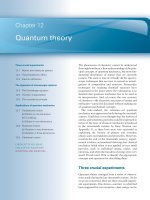
Figure 6A.1  As the reaction advances (represented by motion
from left to right along the horizontal axis) the slope of the
Gibbs energy changes. Equilibrium corresponds to zero slope
at the foot of the valley.

The spontaneity of a reaction at constant temperature and pressure can be expressed in terms of the reaction Gibbs energy:

This equation can be reorganized into

• If ΔrG < 0, the forward reaction is spontaneous.
• If ΔrG > 0, the reverse reaction is spontaneous.



• If ΔrG = 0, the reaction is at equilibrium.

That is,
(6A.2)

We see that ΔrG can also be interpreted as the difference
between the chemical potentials (the partial molar Gibbs energies) of the reactants and products at the current composition of
the reaction mixture.
Because chemical potentials vary with composition, the

slope of the plot of Gibbs energy against extent of reaction,
and therefore the reaction Gibbs energy, changes as the reaction proceeds. The spontaneous direction of reaction lies in
the direction of decreasing G (that is, down the slope of G
plotted against ξ). Thus we see from eqn 6A.2 that the reaction A → B is spontaneous when μA > μ B, whereas the reverse
reaction is spontaneous when μ B > μA. The slope is zero, and
the reaction is at equilibrium and spontaneous in neither
direction, when
∆rG = 0

ΔrG = 0

(b)  Exergonic and endergonic reactions

dG = µ A dnA + µB dnB = − µ A dξ + µB dξ = (µB − µ A )dξ

∆ r G = μB − μ A

ΔrG > 0

Extent of reaction, ξ



 ∂G 
 ∂ξ  = µB − µ A
p ,T

ΔrG < 0
Gibbs energy, G

tially 2.5 mol A is present. What is the composition when
Δξ = +0.5 mol?

A reaction for which ΔrG < 0 is called exergonic (from the
Greek words for work producing). The name signifies that,
because the process is spontaneous, it can be used to drive
another process, such as another reaction, or used to do nonexpansion work. A simple mechanical analogy is a pair of
weights joined by a string (Fig. 6A.2): the lighter of the pair
of weights will be pulled up as the heavier weight falls down.
Although the lighter weight has a natural tendency to move
downward, its coupling to the heavier weight results in it being
raised. In biological cells, the oxidation of carbohydrates act as

Condition of equilibrium  (6A.3)

This condition occurs when μB = μA (Fig. 6A.1). It follows that,
if we can find the composition of the reaction mixture that
ensures μB = μA, then we can identify the composition of the
reaction mixture at equilibrium. Note that the chemical potential is now fulfilling the role its name suggests: it represents
the potential for chemical change, and equilibrium is attained
when these potentials are in balance.

Figure 6A.2  If two weights are coupled as shown here, then
the heavier weight will move the lighter weight in its nonspontaneous direction: overall, the process is still spontaneous.
The weights are the analogues of two chemical reactions: a
reaction with a large negative ΔG can force another reaction
with a smaller ΔG to run in its non-spontaneous direction.


6A  The equilibrium constant  

the heavy weight that drives other reactions forward and results
in the formation of proteins from amino acids, muscle contraction, and brain activity. A reaction for which ΔrG > 0 is called
endergonic (signifying work consuming). The reaction can be
made to occur only by doing work on it, such as electrolysing
water to reverse its spontaneous formation reaction.

reactions
The standard Gibbs energy of the reaction H2 (g) + 12 O2 (g ) →
H2O(l) at 298 K is −237 kJ mol−1, so the reaction is exergonic
and in a suitable device (a fuel cell, for instance) operating at
constant temperature and pressure could produce 237 kJ of
electrical work for each mole of H2 molecules that react. The
reverse reaction, for which ΔrG< = +237 kJ mol−1 is endergonic
and at least 237 kJ of work must be done to achieve it.
Self-test 6A.2  Classify the formation of methane from its ele-

ments as exergonic or endergonic under standard conditions
at 298 K.
Answer: Endergonic

6A.2  The

description of equilibrium

With the background established, we are now ready to see
how to apply thermodynamics to the description of chemical
equilibrium.

(a)  Perfect gas equilibria
When A and B are perfect gases we can use eqn 5A.14b

(μ = μ< + RT ln p, with p interpreted as p/p<) to write
∆ r G = µB − µA = ( µB< + RT ln pB )− ( µA< + RT ln pA )
p
= ∆ r G < + RT ln pB
A



(6A.4)

If we denote the ratio of partial pressures by Q, we obtain
∆ rG = ∆ rG + RT ln Q
<

p
Q = pB
A



(6A.5)

The ratio Q is an example of a ‘reaction quotient’, a quantity we
define more formally shortly. It ranges from 0 when pB = 0 (corresponding to pure A) to infinity when pA = 0 (corresponding
to pure B). The standard reaction Gibbs energy, ΔrG< (Topic
3C), is the difference in the standard molar Gibbs energies of
the reactants and products, so for our reaction
∆ r G < = Gm< (B) − Gm< (A) = μB< − μ A<

Note that in the definition of ΔrG<, the Δr has its normal meaning as the difference ‘products – reactants’. In Topic 3C we saw

that the difference in standard molar Gibbs energies of the
products and reactants is equal to the difference in their standard Gibbs energies of formation, so in practice we calculate
ΔrG< from
∆ r G < = ∆ f G <(B) − ∆ f G <(A)

Brief illustration 6A.2  Exergonic and endergonic

(6A.6)

247

(6A.7)

At equilibrium, ΔrG = 0. The ratio of partial pressures at equilibrium is denoted K, and eqn 6A.5 becomes
0 = ∆ r G < + RT ln K



which rearranges to
RT ln K = − ∆ r G <

p 
K =  pB 
 A  equilibrium

(6A.8)



This relation is a special case of one of the most important equations in chemical thermodynamics: it is the link between tables

of thermodynamic data, such as those in the Resource section,
and the chemically important ‘equilibrium constant’, K (again, a
quantity we define formally shortly).
Brief illustration 6A.3  The equilibrium constant

The standard Gibbs energy of the isomerization of pentane to
2-methylbutane at 298 K, the reaction CH 3(CH 2)3CH3(g) → 
(CH3)2CHCH2CH3(g), is close to −6.7 kJ mol−1 (this is an estimate based on enthalpies of formation; its actual value is not
listed). Therefore, the equilibrium constant for the reaction is
K = e −( −6.7×10

3

J mol −1 )/(8.3145 J K −1 mol −1 )×(298 K )

= e2.7… = 15

Self-test 6A.3  Suppose it is found that at equilibrium the partial pressures of A and B in the gas-phase reaction A ⇌ B are
equal. What is the value of ΔrG Answer: 0

In molecular terms, the minimum in the Gibbs energy, which
corresponds to ΔrG = 0, stems from the Gibbs energy of mixing
of the two gases. To see the role of mixing, consider the reaction A → B. If only the enthalpy were important, then H and
therefore G would change linearly from its value for pure reactants to its value for pure products. The slope of this straight
line is a constant and equal to ΔrG< at all stages of the reaction
and there is no intermediate minimum in the graph (Fig. 6A.3).
However, when the entropy is taken into account, there is an
additional contribution to the Gibbs energy that is given by eqn
5A.16 (ΔmixG = nRT(xA ln xA + xB ln xB)). This expression makes

a U-shaped contribution to the total change in Gibbs energy.


248  6  Chemical equilibrium
values νA = −2, νB = −1, νC = +3, and νD = +1. A stoichio­metric
number is positive for products and negative for reactants.
Then we define the extent of reaction ξ so that, if it changes by
Δξ, then the change in the amount of any species J is νJΔξ.
With these points in mind and with the reaction Gibbs
energy, ΔrG, defined in the same way as before (eqn 6A.1) we
show in the following Justification that the Gibbs energy of
reaction can always be written

Gibbs energy, G

Without
mixing

Including
mixing
0

Mixing
0

Extent of reaction, ξ

Figure 6A.3  If the mixing of reactants and products is ignored,
then the Gibbs energy changes linearly from its initial value
(pure reactants) to its final value (pure products) and the slope

of the line is ΔrG < . However, as products are produced, there
is a further contribution to the Gibbs energy arising from their
mixing (lowest curve). The sum of the two contributions has
a minimum. That minimum corresponds to the equilibrium
composition of the system.

As can be seen from Fig. 6A.3, when it is included there is an
intermediate minimum in the total Gibbs energy, and its position corresponds to the equilibrium composition of the reaction mixture.
We see from eqn 6A.8 that, when ΔrG<> 0, K < 1. Therefore,
at equilibrium the partial pressure of A exceeds that of B,
which means that the reactant A is favoured in the equilibrium.
When ΔrG< < 0, K > 1, so at equilibrium the partial pressure
of B exceeds that of A. Now the product B is favoured in the
equilibrium.
A note on good practice  A common remark is that ‘a reaction is spontaneous if ΔrG < < 0’. However, whether or not a
reaction is spontaneous at a particular composition depends
on the value of ΔrG at that composition, not ΔrG < . It is far
better to interpret the sign of ΔrG < as indicating whether K is
greater or smaller than 1. The forward reaction is spontaneous
(ΔrG < 0) when Q < K and the reverse reaction is spontaneous
when Q > K.

(b)  The general case of a reaction
We can now extend the argument that led to eqn 6A.8 to a
general reaction. First, we note that a chemical reaction may
be expressed symbolically in terms of (signed) stoichiometric
numbers as
0=

∑ J

Symbolic form 

J

J

Reaction Gibbs energy
at an arbitrary stage

∆ r G = ∆ r G < + RT ln Q

Chemical equation  (6A.9)



where J denotes the substances and the νJ are the corresponding
stoichiometric numbers in the chemical equation. In the reaction 2 A + B → 3 C + D, for instance, these numbers have the

(6A.10)

with the standard reaction Gibbs energy calculated from

∑ ∆ G

∆rG< =

f

<

−

Products

∑ ∆ G
f

<

Reactants

Practical
Reaction
implemen­ Gibbs (6A.11a)
energy
tation

where the ν are the (positive) stoichiometric coefficients. More
formally,
∆rG< =

∑ ∆ G
J

f

<

Formal

expression

(J)


J

Reaction
Gibbs
energy

(6A.11b)

where the νJ are the (signed) stoichiometric numbers. The reaction quotient, Q, has the form
Q=

activities of products
activities of reactants



General
form

Reaction
quotient

(6A.12a)

with each species raised to the power given by its stoichio­metric

coefficient. More formally, to write the general expression for Q
we introduce the symbol Π to denote the product of what follows it (just as Σ denotes the sum), and define Q as
Q=

∏a
J

J
J

Definition 



Reaction quotient  (6A.12b)

Because reactants have negative stoichiometric numbers, they
automatically appear as the denominator when the product is
written out explicitly. Recall from Table 5E.1 that, for pure solids
and liquids, the activity is 1, so such substances make no contribution to Q even though they may appear in the chemical equation.
Brief illustration 6A.4  The reaction quotient

Consider the reaction 2 A + 3 B → C + 2 D, in which case
νA = −2, νB = −3, νC = +1, and νD = +2. The reaction quotient is
then
Q = aA−2aB−3aC aD2 =

aC aD2
aA2 aB3

Self-test 6A.4  Write the reaction quotient for A + 2 B → 3 C.
Answer: Q = aC3 /aA aB2


6A  The equilibrium constant  

Justification 6A.1  The dependence of the reaction Gibbs

State

Measure

Approximation
for aJ

Definition

Solute

molality

bJ /bJ<

b< = 1 mol kg−1

molar concentration

[J]/c<

c< = 1 mol dm−3

partial pressure

pJ/p<

p< = 1 bar

energy on the reaction quotient
Consider a reaction with stoichiometric numbers νJ. When
the reaction advances by dξ, the amounts of reactants and
products change by dnJ = νJdξ. The resulting infinitesimal
change in the Gibbs energy at constant temperature and pressure is
dG =





∑µ dn = ∑µ  dξ =  ∑µ   dξ
J

J

J J

J

J J

J

J

It follows that
 ∂G 
=
∆ rG = 
 ∂ξ  p,T

∑ µ
J

Gas phase

In such cases, the resulting expressions are only approximations. The approximation is particularly severe for electrolyte
solutions, for in them activity coefficients differ from 1 even in
very dilute solutions (Topic 5F).
Brief illustration 6A.5  The equilibrium constant

The equilibrium constant for the heterogeneous equilibrium
CaCO3(s) ⇌ CaO(s) + CO2(g) is

J

J

To make progress, we note that the chemical potential of a species J is related to its activity by eqn 5E.9 ( μJ = μJ< + RT ln aJ ).
When this expression is substituted into eqn 6A.11 we obtain

1

aCaO(s ) aCO2 (g )
−1
K = aCaCO
a
a
=
= aCO2 (g )
3 ( s ) CaO( s ) CO2 ( g )
aCaCO3 (s )
1

∆r G <

∆ rG =

∑ μ
J

<
J

+ RT

J

∑ ln a
J

Provided the carbon dioxide can be treated as a perfect gas, we

can go on to write

J

J

Q

∑

= ∆ rG + RT

J ln aJ = ∆ rG + RT ln

<

<

∏

aJ J


J

J

= ∆ rG < + RT ln Q
In the second line we use first a ln x = ln x a and then ln x + ln
y + … = ln xy…, so

∑
i


ln xi = ln 



xi 


i



aJ 
 equilibrium

∏
J

J



K = pCO2 /p <
and conclude that in this case the equilibrium constant is the
numerical value of the decomposition vapour pressure of calcium carbonate.
Self-test 6A.5  Write the equilibrium constant for the reaction

N2(g) + 3 H2(g) ⇌ 2 NH3(g), with the gases treated as perfect.

2
3 = p2
3
Answer: K = aNH
/aN2 aH
p <2 /pN2 pH
NH

∏

3

Now we conclude the argument, starting from eqn 6A.10. At
equilibrium, the slope of G is zero: ΔrG = 0. The activities then
have their equilibrium values and we can write

K =


249

Definition 

Equilibrium constant  (6A.13)

This expression has the same form as Q but is evaluated using
equilibrium activities. From now on, we shall not write the

‘equilibrium’ subscript explicitly, and will rely on the context
to make it clear that for K we use equilibrium values and for
Q we use the values at the specified stage of the reaction. An
equilibrium constant K expressed in terms of activities (or
fugacities) is called a thermodynamic equilibrium constant.
Note that, because activities are dimensionless numbers, the
thermodynamic equilibrium constant is also dimensionless. In
elementary applications, the activities that occur in eqn 6A.13
are often replaced as follows:

2

3

2

At this point we set ΔrG = 0 in eqn 6A.10 and replace Q by K.
We immediately obtain
∆ r G < = − RT ln K Thermodynamic equilibrium constant  (6A.14)
This is an exact and highly important thermodynamic relation, for it enables us to calculate the equilibrium constant of
any reaction from tables of thermodynamic data, and hence to
predict the equilibrium composition of the reaction mixture. In
Topic 15F we see that the right-hand side of eqn 6A.14 may be
expressed in terms of spectroscopic data for gas-phase species;
so this expression also provides a link between spectroscopy
and equilibrium composition.
Example 6A.1  Calculating an equilibrium constant

Calculate the equilibrium constant for the ammonia synthesis
reaction, N2(g) + 3 H2(g) ⇌ 2 NH3(g), at 298 K and show how K

is related to the partial pressures of the species at equilibrium


250  6  Chemical equilibrium
when the overall pressure is low enough for the gases to be
treated as perfect.

which opens the way to making approximations to obtain its
numerical value.

Method  Calculate the standard reaction Gibbs energy from

Answer  The equilibrium constant is obtained from eqn 6A.14
in the form

eqn 6A.10 and convert it to the value of the equilibrium constant by using eqn 6A.14. The expression for the equilibrium
constant is obtained from eqn 6A.13, and because the gases are
taken to be perfect, we replace each activity by the ratio pJ/p < ,
where pJ is the partial pressure of species J.
Answer  The standard Gibbs energy of the reaction is

∆ rG < = 2∆ f G < (NH3 , g ) − {∆ f G < (N2 , g ) + 3∆ f G < (H2 , g )}
= 2∆ f G < (NH3 , g ) = 2 × (−16.45kJmol −1 )

ln K = −
=−

1.1808 × 105 Jmol −1
∆ rG <
=−

RT
(8.3145 JK −1 mol −1 ) × (2300 K )
1.1808 × 105
= −6.17…
8.3145 × 2300

It follows that K = 2.08 × 10 −3. The equilibrium composition
can be expressed in terms of α by drawing up the following
table:

Then,
2 × (−1.645 × 104 Jmol −1)
2 × 1.645 × 104
=
ln K = −
= 13.2…
(8.3145 JK −1 mol −1) × (298 K) 8.3145 × 298
Hence, K = 5.8 × 105. This result is thermodynamically exact.
The thermodynamic equilibrium constant for the reaction is
K=

2
aNH
3
aN2 aH3 2

and this ratio has the value we have just calculated. At low
overall pressures, the activities can be replaced by the ratios
pJ/p < and an approximate form of the equilibrium constant is
K=

2
pNH
p <2
( pNH3 /p < )2
3
<
< 3 =
( pN2 /p )( pH2 /p )
pN2 pH3 2

H2O

H2

+ 12 O2

Initial amount

n

0

0

Change to reach
equilibrium

−αn

+αn

+ 12 αn

Amount at
equilibrium

(1 − α)n

αn

1
αn
2

Mole fraction, xJ

1− α
1+ 12 α

α
1+ 12

1α
2
1+ 21 α

Partial pressure, pJ

(1−α ) p

1+ 12 α

αp
1+ 12

1 αp
2
1+ 12 α

Total: (1+ 12 α )n

where, for the entries in the last row, we have used pJ = xJp (eqn
1A.8). The equilibrium constant is therefore

Self-test 6A.6  Eva luate t he equi librium constant for

N2O4(g) ⇌ 2 NO2(g) at 298 K.

K=

Answer: K = 0.15

Example 6A.2  Estimating the degree of dissociation

at equilibrium
The degree of dissociation (or extent of dissociation, α) is
defined as the fraction of reactant that has decomposed; if
the initial amount of reactant is n and the amount at equilibrium is neq, then α = (n − neq)/n. The standard reaction Gibbs
energy for the decomposition H 2O(g) → H 2(g) + 12 O2(g) is
+118.08 kJ mol−1 at 2300 K. What is the degree of dissociation

of H2O at 2300 K and 1.00 bar?
Method  The equilibrium constant is obtained from the standard Gibbs energy of reaction by using eqn 6A.11, so the task is
to relate the degree of dissociation, α, to K and then to find its
numerical value. Proceed by expressing the equilibrium compositions in terms of α, and solve for α in terms of K. Because
the standard reaction Gibbs energy is large and positive, we
can anticipate that K will be small, and hence that α ≪ 1,

pH2 pO1/22
α 3/2 p1/2
=
pH2 O
(1 − α )(2 + α )1/2

In this expression, we have written p in place of p/p <, to simplify its appearance. Now make the approximation that α ≪ 1,
and hence obtain
K≈

α 3/2 p1/2
21/2

Under the stated condition, p = 1.00 bar (that is, p/p < = 1.00),
so α ≈ (21/2K)2/3 = 0.0205. That is, about 2 per cent of the water
has decomposed.
A note on good practice  Always check that the approximation is consistent with the final answer. In this case α ≪ 1,
in accord with the original assumption.
Self-test 6A.7  Given that the standard Gibbs energy of reaction at 2000 K is +135.2 kJ mol−1 for the same reaction, suppose
that steam at 200 kPa is passed through a furnace tube at that
temperature. Calculate the mole fraction of O2 present in the
output gas stream.
Answer: 0.00221

6A  The equilibrium constant  

(c)  The relation between equilibrium

 c < RT 
K = Kc ×  < 
 p 

constants

Equilibrium constants in terms of activities are exact, but it is
often necessary to relate them to concentrations. Formally, we
need to know the activity coefficients, and then to use aJ = γJxJ,
aJ = γJbJ/b<, or aJ = [J]/c<, where xJ is a mole fraction, bJ is a
molality, and [J] is a molar concentration. For example, if we
were interested in the composition in terms of molality for an
equilibrium of the form A + B ⇌ C + D, where all four species
are solutes, we would write
K=

aC aD γ Cγ D bC bD
=
×
= Kγ Kb
aA aB γ Aγ B bA bB


(6A.15)

The activity coefficients must be evaluated at the equilibrium
composition of the mixture (for instance, by using one of the
Debye–Hückel expressions, Topic 5F), which may involve a
complicated calculation, because the activity coefficients are
known only if the equilibrium composition is already known.
In elementary applications, and to begin the iterative calculation of the concentrations in a real example, the assumption is
often made that the activity coefficients are all so close to unity
that Kγ  = 1. Then we obtain the result widely used in elementary
chemistry that K ≈ Kb, and equilibria are discussed in terms of
molalities (or molar concentrations) themselves.
A special case arises when we need to express the equilibrium constant of a gas-phase reaction in terms of molar concentrations instead of the partial pressures that appear in the
thermodynamic equilibrium constant. Provided we can treat
the gases as perfect, the pJ that appear in K can be replaced by
[J]RT, and
K=

∏

aJ =
J

J

=

∏
J

J

 pJ 
 p <  =
 RT 
<


∏[J] × ∏  p
J

J

J

 RT 
[J]  < 
p 

∏
J

J

J

J



(Products can always be factorized like that: abcdef is the same

as abc × def.) The (dimensionless) equilibrium constant Kc is
defined as
Kc =

∏
J

 [J] 
 c < 

J

Definition 

Kc for gas-phase reactions  (6A.16)



It follows that
K = Kc ×

∏
J

 c < RT 
 p < 

J

(6A.17a)

If now we write Δν =∑JνJ, which is easier to think of as
ν(products) – ν(reactants), then the relation between K and Kc
for a gas-phase reaction is

∆

Relation between K and
Kc for gas-phase reactions



251

(6A.17b)

The term in parentheses works out as T/(12.03 K).
Brief illustration 6A.6  The relation between equilibrium

constants
For the reaction N2(g) + 3 H2(g) → 2 NH3(g), Δν = 2 − 4 = −2, so
 T 
K = Kc × 
 12.03 K 

−2

 12.03 K 

= Kc × 
 T 

2

At 298.15 K the relation is
2

K
 12.03 K 
= c
K = Kc × 
 298.15 K  614.2
so Kc = 614.2K. Note that both K and Kc are dimensionless.
Self-test 6A.8  Find the relation between K and Kc for the equilibrium H2 (g) + 12 O2 (g ) → H2O(l) at 298K.

Answer: K c = 123K

(d)  Molecular interpretation of the

equilibrium constant

Deeper insight into the origin and significance of the equilibrium constant can be obtained by considering the Boltzmann
distribution of molecules over the available states of a system
composed of reactants and products (Foundations B). When
atoms can exchange partners, as in a reaction, the available
states of the system include arrangements in which the atoms
are present in the form of reactants and in the form of products: these arrangements have their characteristic sets of energy
levels, but the Boltzmann distribution does not distinguish
between their identities, only their energies. The atoms distribute themselves over both sets of energy levels in accord with

the Boltzmann distribution (Fig. 6A.4). At a given temperature,
there will be a specific distribution of populations, and hence a
specific composition of the reaction mixture.
It can be appreciated from the illustration that, if the reactants and products both have similar arrays of molecular
energy levels, then the dominant species in a reaction mixture at equilibrium will be the species with the lower set of
energy levels. However, the fact that the Gibbs energy occurs
in the expression is a signal that entropy plays a role as well as
energy. Its role can be appreciated by referring to Fig. 6A.4. In
Fig. 6A.4b we see that, although the B energy levels lie higher
than the A energy levels, in this instance they are much more
closely spaced. As a result, their total population may be considerable and B could even dominate in the reaction mixture at
equilibrium. Closely spaced energy levels correlate with a high


252  6  Chemical equilibrium
B

(a)

Boltzmann
distribution

Population, P

A

Note that a positive reaction enthalpy results in a lowering of
the equilibrium constant (that is, an endothermic reaction can
be expected to have an equilibrium composition that favours
the reactants). However, if there is positive reaction entropy,

then the equilibrium composition may favour products, despite
the endothermic character of the reaction.

B

Energy, E

Energy, E

A

Boltzmann
distribution

Brief illustration 6A.7  Contributions to K

In Example 6A.1 it is established that Δ rG < = −33.0 kJ mol−1
for the reaction N2(g) + 3 H 2(g) ⇌ 2 NH 3(g) at 298 K. From
the tables of data in the Resource section, we can find that
ΔrH < = −92.2 kJ mol−1 and ΔrS < = −198.8 J K−1 mol−1. The contributions to K are therefore

Population, P

(b)

Figure 6A.4  The Boltzmann distribution of populations over
the energy levels of two species A and B with similar densities
of energy levels. The reaction A → B is endothermic in this
example. (a) The bulk of the population is associated with the
species A, so that species is dominant at equilibrium. (b) Even

though the reaction A → B is endothermic, the density of
energy levels in B is so much greater than that in A that the
population associated with B is greater than that associated
with A, so B is dominant at equilibrium.

K = e −( −9.22 × 10

× e( −198.8 J K

r

/RT

<

e∆ S
r

/R

<

mol −1 )/(8.3145 J K −1 mol −1 )

We see that the exothermic character of the reaction encourages the formation of products (it results in a large increase in
entropy of the surroundings) but the decrease in entropy of
the system as H atoms are pinned to N atoms opposes their
formation.
Self-test 6A.9  Analyse the equilibrium N2O 4(g) ⇌ 2 NO2(g)

similarly.

Answer: K = e−26.7… × e21.1…; enthalpy opposes, entropy encourages

(6A.18)



J mol −1 )/(8.3145 J K −1 mol −1 ) × (298 K )
−1

= e37.2… × e −23.9…

entropy (Topic 15E), so in this case we see that entropy effects
dominate adverse energy effects. This competition is mirrored
in eqn 6A.14, as can be seen most clearly by using ΔrG<  =
ΔrH<− TΔrS< and writing it in the form
K = e− ∆ H

4

Checklist of concepts
☐1.The reaction Gibbs energy is the slope of the plot of
Gibbs energy against extent of reaction.
☐2.Reactions are either exergonic or endergonic.
☐3.The reaction Gibbs energy depends logarithmically on
the reaction quotient.

☐4.When the reaction Gibbs energy is zero the reaction
quotient has a value called the equilibrium constant.

☐5.Under ideal conditions, the thermodynamic equilibrium constant may be approximated by expressing it in
terms of concentrations and partial pressures.

Checklist of equations
Property

Equation

Comment

Equation number

Reaction Gibbs energy

ΔrG = (∂G/∂ξ)p,T

Definition

6A.1

Reaction Gibbs energy

ΔrG = ΔrG< + RT ln Q

Standard reaction Gibbs energy

∆rG < =

6A.10

∑ ∆ G − ∑ ∆ G
=
∑ ∆ G (J)
<

f

Products

J f

J

f

Reactants

<

<

ν are positive; νJ are signed

6A.11


6A  The equilibrium constant  

253

Property

Equation

Comment

Equation number

Reaction quotient


Q = Π aJ J
J

Definition; evaluated at arbitrary stage of reaction

6A.12

Thermodynamic equilibrium constant


 
K =  Π aJ J 
J
 equilibrium

Definition

6A.13

Equilibrium constant

ΔrG< = −RT ln K

Relation between K and Kc

K = Kc(c
6A.14
Gas-phase reactions; perfect gases

6A.17b


6B  The response of equilibria
to the conditions
Contents
6B.1 

The response to pressure

6B.2 

The response to temperature

Brief illustration 6B.1: Le Chatelier’s principle
The van ’t Hoff equation
Example 6B.1: Measuring a reaction enthalpy
(b) The value of K at different temperatures
Brief illustration 6B.2: The temperature

dependence of K
(a)

Checklist of concepts
Checklist of equations

254
255
255
256
257
257
257
258
258

➤➤ Why do you need to know this material?
Chemists, and chemical engineers designing a chemical
plant, need to know how an equilibrium will respond to
changes in the conditions, such as a change in pressure or
temperature. The variation with temperature also provides
a way to determine the enthalpy and entropy of a reaction.

➤➤ What is the key idea?
A system at equilibrium, when subjected to a disturbance,
responds in a way that tends to minimize the effect of the
disturbance.

➤➤ What do you need to know already?
This Topic builds on the relation between the equilibrium

constant and the standard Gibbs energy of reaction (Topic
6A). To express the temperature dependence of K it draws
on the Gibbs–Helmholtz equation (Topic 3D).

The equilibrium constant for a reaction is not affected by the
presence of a catalyst or an enzyme (a biological catalyst). As
explained in detail in Topics 20H and 22C, catalysts increase the
rate at which equilibrium is attained but do not affect its position. However, it is important to note that in industry reactions
rarely reach equilibrium, partly on account of the rates at which
reactants mix. The equilibrium constant is also independent
of pressure, but as we shall see, that does not necessarily mean

that the composition at equilibrium is independent of pressure.
The equilibrium constant does depend on the temperature in
a manner that can be predicted from the standard reaction
enthalpy.

6B.1  The

response to pressure

The equilibrium constant depends on the value of ΔrG<, which
is defined at a single, standard pressure. The value of ΔrG<, and
hence of K, is therefore independent of the pressure at which
the equilibrium is actually established. In other words, at a
given temperature K is a constant.
The conclusion that K is independent of pressure does not
necessarily mean that the equilibrium composition is independent of the pressure, and the effect depends on how the
pressure is applied.
The pressure within a reaction vessel can be increased by

injecting an inert gas into it. However, so long as the gases are
perfect, this addition of gas leaves all the partial pressures of the
reacting gases unchanged: the partial pressures of a perfect gas
is the pressure it would exert if it were alone in the container, so
the presence of another gas has no effect. It follows that pressurization by the addition of an inert gas has no effect on the
equilibrium composition of the system (provided the gases are
perfect).
Alternatively, the pressure of the system may be increased by
confining the gases to a smaller volume (that is, by compression). Now the individual partial pressures are changed but
their ratio (as it appears in the equilibrium constant) remains
the same. Consider, for instance, the perfect gas equilibrium
A ⇌ 2 B, for which the equilibrium constant is
K=

pB2
pA p <



The right-hand side of this expression remains constant only
if an increase in pA cancels an increase in the square of pB. This
relatively steep increase of pA compared to pB will occur if the
equilibrium composition shifts in favour of A at the expense of
B. Then the number of A molecules will increase as the volume
of the container is decreased and its partial pressure will rise


6B  The response of equilibria to the conditions  

255

Brief illustration 6B.1  Le Chatelier’s principle

To predict the effect of an increase in pressure on the composition of the ammonia synthesis at equilibrium, Example 6A.1,
we note that the number of gas molecules decreases (from 4
to 2). So, Le Chatelier’s principle predicts that an increase in
pressure will favour the product. The equilibrium constant is
(b)

Figure 6B.1  When a reaction at equilibrium is compressed
(from a to b), the reaction responds by reducing the number
of molecules in the gas phase (in this case by producing the
dimers represented by the linked spheres).

A system at equilibrium, when subjected to a
disturbance, responds in a way that tends to
minimize the effect of the disturbance.

Le Chatelier’s
principle

more rapidly than can be ascribed to a simple change in volume
alone (Fig. 6B.1).
The increase in the number of A molecules and the corresponding decrease in the number of B molecules in the equilibrium A ⇌ 2 B is a special case of a principle proposed by the
French chemist Henri Le Chatelier, which states that:

The principle implies that, if a system at equilibrium is compressed, then the reaction will adjust so as to minimize the
increase in pressure. This it can do by reducing the number of
particles in the gas phase, which implies a shift A ← 2 B.
To treat the effect of compression quantitatively, we suppose

that there is an amount n of A present initially (and no B). At
equilibrium the amount of A is (1 − α)n and the amount of B is
2αn, where α is the degree of dissociation of A into 2B. It follows that the mole fractions present at equilibrium are
xA =

(1− α )n
1− α
=
(1− α )n + 2αn 1+ α

xB =

2α
1+ α

The equilibrium constant for the reaction is

Self-test 6B.1  Predict the effect of a tenfold pressure

increase on the equilibrium composition of the reaction
3 N2(g) + H2(g) ⇌ 2 N3H(g).
Answer: 100-fold increase in K x

1

100
0.8
0.6

10

0.4

1

0.2

0.1
0

0

which rearranges to
1/2

(6B.1)



This formula shows that, even though K is independent of
pressure, the amounts of A and B do depend on pressure (Fig.
6B.2). It also shows that as p is increased, α decreases, in accord
with Le Chatelier’s principle.

4

8
Pressure, p/p<

12

16

Figure 6B.2  The pressure dependence of the degree of
dissociation, α, at equilibrium for an A(g) ⇌ 2 B(g) reaction for
different values of the equilibrium constant K. The value α = 0
corresponds to pure A; α = 1 corresponds to pure B

6B.2  The

p2
x 2 p2
4α 2 ( p/p < )
K = B< = B < =
pA p
x A pp
1− α 2



1
α =
 1 + 4 p/Kp < 

2
2
2
pNH
p < x NH
p2 p <2 x NH

p <2
p <2
3
3
3
=
=
= Kx × 2
3
3
4
3
2
pN2 pH2
x N 2 x H2 p
x N 2 x H2 p
p

where K x is the part of the equilibrium constant expression
that contains the equilibrium mole fractions of reactants and
products (note that, unlike K itself, K x is not an equilibrium
constant). Therefore, doubling the pressure must increase K x
by a factor of 4 to preserve the value of K.

Extent of dissociation, α

(a)

K=

response to temperature

Le Chatelier’s principle predicts that a system at equilibrium
will tend to shift in the endothermic direction if the temperature is raised, for then energy is absorbed as heat and the rise
in temperature is opposed. Conversely, an equilibrium can be
expected to shift in the exothermic direction if the temperature
is lowered, for then energy is released and the reduction in temperature is opposed. These conclusions can be summarized as
follows:
Exothermic reactions: increased temperature favours the
reactants.


256  6  Chemical equilibrium
Endothermic reactions: increased temperature favours
the products.
We shall now justify these remarks thermodynamically and see
how to express the changes quantitatively.

(a)  The van ’t Hoff equation
The van ’t Hoff equation, which is derived in the following
Justification, is an expression for the slope of a plot of the equilibrium constant (specifically, ln K) as a function of temperature. It may be expressed in either of two ways:
van ‘t Hoff equation  (6B.2a)



d ln K
∆ H<
=− r
d(1/T )
R

Alternative
version 

van ‘t Hoff
equation

(6B.2b)

Justification 6B.1  The van ’t Hoff equation

From eqn 6A.14, we know that
∆ rG <
RT

Differentiation of ln K with respect to temperature then gives
1 d(∆ rG < /T )
d ln K
=−
dT
dT
R

The differentials are complete (that is, they are not partial
derivatives) because K and ΔrG < depend only on temperature,
not on pressure. To develop this equation we use the Gibbs–
Helmholtz equation (eqn 3D.10, d(ΔG/T) = −ΔH/T 2) in the
form

A

A

B



where Δ rH < is the standard reaction enthalpy at the temperature T. Combining the two equations gives the van ’t
Hoff equation, eqn 6B.2a. The second form of the equation is
obtained by noting that
1
d(1/T )
= − 2 , so dT = −T 2d(1/T )
dT
T

It follows that eqn 6B.2a can be rewritten as
−

B

<

d ln K
∆H
= r
T 2d(1/ T ) RT 2

(a)

High temperature

High temperature

Exothermic

d(∆ rG /T )
∆H
=− r
dT
R
<

Endothermic

ln K = −

Energy, E

d ln K ∆ r H <
=
dT
RT 2

conditions (ΔrH< < 0). A negative slope means that ln K, and
therefore K itself, decreases as the temperature rises. Therefore,
as asserted above, in the case of an exothermic reaction the
equilibrium shifts away from products. The opposite occurs in
the case of endothermic reactions.
Insight into the thermodynamic basis of this behaviour

comes from the expression ΔrG< = ΔrH< – TΔrS< written in the
form –ΔrGof the surroundings and favours the formation of products.
When the temperature is raised, –ΔrHincreasing entropy of the surroundings has a less important
role. As a result, the equilibrium lies less to the right. When
the reaction is endothermic, the principal factor is the increasing entropy of the reaction system. The importance of the
un­favourable change of entropy of the surroundings is reduced
if the temperature is raised (because then ΔrHand the reaction is able to shift towards products.
These remarks have a molecular basis that stems from the
Boltzmann distribution of molecules over the available energy
levels (Foundations B, and in more detail in Topic 15F). The
typical arrangement of energy levels for an endothermic reaction is shown in Fig. 6B.3a. When the temperature is increased,
the Boltzmann distribution adjusts and the populations change
as shown. The change corresponds to an increased population of the higher energy states at the expense of the population of the lower energy states. We see that the states that arise
from the B molecules become more populated at the expense
of the A molecules. Therefore, the total population of B states
increases, and B becomes more abundant in the equilibrium
mixture. Conversely, if the reaction is exothermic (Fig. 6B.3b),

Low temperature

Population, P

(b)

Low temperature

Population, P

<

which simplifies into eqn 6B.2b.

Equation 6B.2a shows that d ln K/dT < 0 (and therefore that
dK/dT < 0) for a reaction that is exothermic under standard

Figure 6B.3  The effect of temperature on a chemical
equilibrium can be interpreted in terms of the change in the
Boltzmann distribution with temperature and the effect of that
change in the population of the species. (a) In an endothermic
reaction, the population of B increases at the expense of A as
the temperature is raised. (b) In an exothermic reaction, the
opposite happens.


6B  The response of equilibria to the conditions  
then an increase in temperature increases the population of the
A states (which start at higher energy) at the expense of the B
states, so the reactants become more abundant.
The temperature dependence of the equilibrium constant
provides a non-calorimetric method of determining ΔrH<. A
drawback is that the reaction enthalpy is actually temperaturedependent, so the plot is not expected to be perfectly linear.
However, the temperature dependence is weak in many cases,
so the plot is reasonably straight. In practice, the method is not
very accurate, but it is often the only method available.

The data below show the temperature variation of the equilibrium constant of the reaction Ag2CO3(s) ⇌ Ag2O(s) + CO2(g).
Calculate the standard reaction enthalpy of the decomposition.

K

350

400

450

500

3.98 × 10−4

1.41 × 10−2

1.86 × 10−1

1.48

enthalpy can be assumed to be independent of temperature,
a plot of –ln K against 1/T should be a straight line of slope
ΔrH< /R.

Answer  We draw up the following table:

350

400

450

2.86

2.50

2.22

2.00

–ln K

6.83

4.26

1.68

−0.39

To find the value of the equilibrium constant at a temperature
T2 in terms of its value K1 at another temperature T1, we integrate eqn 6B.2b between these two temperatures:
1
R

∫

1/T2

1/T1

∆ r H < d(1/T )

(6B.4)



If we suppose that ΔrH< varies only slightly with temperature
over the temperature range of interest, then we may take it outside the integral. It follows that
ln K 2 − ln K1 = −

∆r H <  1 1 
−
R  T2 T1 

Temperature
dependence of K

(6B.5)

To estimate the equilibrium constant or the synthesis of
ammonia at 500 K from its value at 298 K (6.1 × 105 for the
reaction written as N2(g) + 3 H 2(g) ⇌ 2 NH 3(g)) we use the
standard reaction enthalpy, which can be obtained from Table
2C.2 in the Resource section by using ΔrH < = 2Δf H < (NH3,g)
and assume that its value is constant over the range of temperatures. Then, with ΔrH< = −92.2 kJ mol−1, from eqn 6B.3 we
find

6
–ln K

Answer: −200 kJ mol−1

Brief illustration 6B.2  The temperature dependence of K

8

4

2

2

Self-test 6B.2  The equilibrium constant of the reaction
2 SO2(g) + O2(g) ⇌ 2 SO3(g) is 4.0 × 1024 at 300 K, 2.5 × 1010 at
500 K, and 3.0 × 10 4 at 700 K. Estimate the reaction enthalpy
at 500 K.

500

(103 K)/T

0

∆ r H < = (+9.6 × 103 K ) × R = +80 kJmol −1

ln K 2 − ln K1 = −

Method  It follows from eqn 6B.2b that, provided the reaction

T/K

These points are plotted in Fig. 6B.4. The slope of the graph is
+9.6 × 103, so

(b)  The value of K at different temperatures

Example 6B.1  Measuring a reaction enthalpy

T/K

257

2.2

2.4

(103 K)/T

2.6

2.8

Figure 6B.4  When –ln K is plotted against 1/T, a straight
line is expected with slope equal to ΔrH < /R if the standard
reaction enthalpy does not vary appreciably with
temperature. This is a non-calorimetric method for the
measurement of reaction enthalpies.

3

 −9.22 ×104 Jmol −1   1

1 
ln K 2 = ln(6.1 × 105 ) − 
×
−
−1
−1   500 K
298
K 
 8.3145 JK mol  
= −1.7…

It follows that K 2 = 0.18, a lower value than at 298 K, as expected
for this exothermic reaction.
Self-test 6B.3  The equilibrium constant for N 2 O 4 (g) ⇌ 
2 NO2(g) was calculated in Self-test 6A.6. Estimate its value at
100 °C.
Answer: 15


258  6  Chemical equilibrium

Checklist of concepts
☐1.The thermodynamic equilibrium constant is independent of pressure.
☐2.The response of composition to changes in the conditions is summarized by Le Chatelier’s principle.

☐3.The dependence of the equilibrium constant on the
temperature is expressed by the van ’t Hoff equation
and can be explained in terms of the distribution of
molecules over the available states.

Checklist of equations
Property

Equation

van ’t Hoff equation

d ln K/dT = ΔrH
Temperature dependence of equilibrium constant

Comment

Equation number
6B.2a

d ln K/d(1/T) = −ΔrH
Alternative version

6B.2b

ln K2 − ln K1 = −(ΔrH
ΔrH< assumed constant

6B.5


6C  Electrochemical cells

Contents
6C.1 

Half-reactions and electrodes
Brief illustration 6C.1 Redox couples
Brief illustration 6C.2 The reaction quotient

6C.2 

Varieties of cells
Liquid junction potentials
(b) Notation
Brief illustration 6C.3 Cell notation
(a)

6C.3 

The cell potential
Brief illustration 6C.4 The cell reaction
(a) The Nernst equation
Brief illustration 6C.5 The reaction Gibbs energy
Brief illustration 6C.6 The Nernst equation
(b) Cells at equilibrium
Brief illustration 6C.7 Equilibrium constants

6C.4 

The determination of thermodynamic
functions
Brief illustration 6C.8 The reaction Gibbs energy

Example 6C.1 Using the temperature coefficient
of the cell potential

Checklist of concepts
Checklist of equations

259
260
260
260
261
261
261
261
262
262
263
264
264
264
264
264
265
265
266

➤➤ Why do you need to know this material?
One very special case of the material treated in Topic
6B that has enormous fundamental, technological, and
economic significance concerns reactions that take place

in electrochemical cells. Moreover, the ability to make very
precise measurements of potential differences (‘voltages’)
means that electrochemical methods can be used to
determine thermodynamic properties of reactions that
may be inaccessible by other methods.

➤➤ What is the key idea?
The electrical work that a reaction can perform at constant
pressure and temperature is equal to the reaction Gibbs
energy.

➤➤ What do you need to know already?
This Topic develops the relation between the Gibbs energy
and non-expansion work (Topic 3C). You need to be aware

of how to calculate the work of moving a charge through
an electrical potential difference (Topic 2A). The equations
make use of the definition of the reaction quotient Q and
the equilibrium constant K (Topic 6A).

An electrochemical cell consists of two electrodes, or metallic conductors, in contact with an electrolyte, an ionic conductor (which may be a solution, a liquid, or a solid). An electrode
and its electrolyte comprise an electrode compartment. The
two electrodes may share the same compartment. The various
kinds of electrode are summarized in Table 6C.1. Any ‘inert
metal’ shown as part of the specification is present to act as a
source or sink of electrons, but takes no other part in the reaction other than acting as a catalyst for it. If the electrolytes are
different, the two compartments may be joined by a salt bridge,
which is a tube containing a concentrated electrolyte solution
(for instance, potassium chloride in agar jelly) that completes
the electrical circuit and enables the cell to function. A galvanic

cell is an electrochemical cell that produces electricity as a
result of the spontaneous reaction occurring inside it. An electrolytic cell is an electrochemical cell in which a non-spontan­
eous reaction is driven by an external source of current.

6C.1  Half-reactions

and electrodes

It will be familiar from introductory chemistry courses that oxidation is the removal of electrons from a species, a reduction is
the addition of electrons to a species, and a redox reaction is a
Table 6C.1  Varieties of electrode
Electrode
type

Designation

Redox
couple

Half-reaction

Metal/
metal
ion

M(s)|M+(aq)

M+/M

M+(aq) + e− → M(s)

Gas

Pt(s)|X2(g)|X+(aq)

X+/X2

X + (aq) + e − → 12 X 2 (g)

Pt(s)|X2(g)|X−(aq)

X2/X−

1
2

Metal/
M(s)|MX(s)|X−(aq)
insoluble
salt
Redox

X 2 (g) + e − → X − (aq)

MX/M,X− MX(s) + e− → M(s) + X−(aq)

Pt(s)|M+(aq),M2+(aq) M2+/M+

M2+(aq) + e− → M+(aq)

260  6  Chemical equilibrium
reaction in which there is a transfer of electrons from one species to another. The electron transfer may be accompanied by
other events, such as atom or ion transfer, but the net effect is
electron transfer and hence a change in oxidation number of
an element. The reducing agent (or reductant) is the electron
donor; the oxidizing agent (or oxidant) is the electron acceptor. It should also be familiar that any redox reaction may be
expressed as the difference of two reduction half-reactions,
which are conceptual reactions showing the gain of electrons.
Even reactions that are not redox reactions may often be
expressed as the difference of two reduction half-reactions. The
reduced and oxidized species in a half-reaction form a redox
couple. In general we write a couple as Ox/Red and the corres­
ponding reduction half-reaction as
Ox + e – → Red

(6C.1)

The reduction and oxidation processes responsible for the
overall reaction in a cell are separated in space: oxidation takes
place at one electrode and reduction takes place at the other.
As the reaction proceeds, the electrons released in the oxidation Red1 → Ox1 + ν e− at one electrode travel through the
external circuit and re-enter the cell through the other electrode. There they bring about reduction Ox2 + ν e− → Red2.
The electrode at which oxidation occurs is called the anode;
the electrode at which reduction occurs is called the cathode.
In a galvanic cell, the cathode has a higher potential than the
anode: the species undergoing reduction, Ox2, withdraws electrons from its electrode (the cathode, Fig. 6C.1), so leaving a
relative positive charge on it (corresponding to a high potential). At the anode, oxidation results in the transfer of electrons
to the electrode, so giving it a relative negative charge (corres­
ponding to a low potential).

Brief illustration 6C.1  Redox couples

The dissolution of silver chloride in water AgCl(s) → 
Ag + (aq) + Cl − (aq), which is not a redox reaction, can be
expressed as the difference of the following two reduction
half-reactions:
AgCl(s) + e − → Ag(s) + Cl − (aq)
Ag + (aq) + e − → Ag(s)
The redox couples are AgCl/Ag,Cl− and Ag+/Ag, respectively.
Self-test 6C.1  Express the formation of H 2O from H 2 and O2
in acidic solution (a redox reaction) as the difference of two
reduction half-reactions.
Answer: 4 H+(aq) + 4 e− → 2 H2(g), O2(g) + 4 H+(aq) + 4 e− → 2 H2O(l)

We shall often find it useful to express the composition of an
electrode compartment in terms of the reaction quotient, Q,
for the half-reaction. This quotient is defined like the reaction
quotient for the overall reaction (Topic 6A, Q = Π aJ ), but the
J
electrons are ignored because they are stateless.
J

6C.2  Varieties

of cells

The simplest type of cell has a single electrolyte common to
both electrodes (as in Fig. 6C.1). In some cases it is necessary to immerse the electrodes in different electrolytes, as
in the ‘Daniell cell’ in which the redox couple at one electrode is Cu2+/Cu and at the other is Zn2+/Zn (Fig. 6C.2). In

an electrolyte concentration cell, the electrode compartments are identical except for the concentrations of the electrolytes. In an electrode concentration cell the electrodes
themselves have different concentrations, either because they
are gas electrodes operating at different pressures or because
they are amalgams (solutions in mercury) with different
concentrations.

–

Anode

+

Electrons
Cathode

Brief illustration 6C.2  The reaction quotient

The reaction quotient for the reduction of O2 to H 2O in acid
solution, O2(g) + 4 H+(aq) + 4 e− → 2 H2O(l), is
Q=

aH2 2 O
p<
≈ 4
4
aH+ aO2 aH+ pO2

The approximations used in the second step are that the activity of water is 1 (because the solution is dilute) and the oxygen
behaves as a perfect gas, so aO2 ≈ pO2 /p < .
Self-test 6C.2  Write the half-reaction and the reaction quotient for a chlorine gas electrode.

2
<
/pCl2
Answer: Cl 2(g) + 2 e− → 2 Cl− (aq), Q ≈ aCl
− p

Oxidation

Reduction

Figure 6C.1  When a spontaneous reaction takes place
in a galvanic cell, electrons are deposited in one electrode
(the site of oxidation, the anode) and collected from
another (the site of reduction, the cathode), and so there
is a net flow of current which can be used to do work.
Note that the + sign of the cathode can be interpreted as
indicating the electrode at which electrons enter the
cell, and the – sign of the anode is where the electrons
leave the cell.


6C  Electrochemical cells  

–

261

(b)  Notation

+

We use the following notation for cells:

Porous
pot
Zinc
Zinc sulfate
solution

|

A phase boundary

Copper



A liquid junction

Copper(II) sulfate
solution

||

An interface for which it is assumed that the
junction potential has been eliminated

Figure 6C.2  One version of the Daniell cell. The copper
electrode is the cathode and the zinc electrode is the anode.
Electrons leave the cell from the zinc electrode and enter it

again through the copper electrode.

(a)  Liquid junction potentials

A cell in which two electrodes share the same electrolyte is
Pt(s) H2 (g) HCl(aq) AgCl Ag(s)
The cell in Fig. 6C.2 is denoted

In a cell with two different electrolyte solutions in contact, as in
the Daniell cell, there is an additional source of potential difference across the interface of the two electrolytes. This potential
is called the liquid junction potential, Elj. Another example of
a junction potential is that between different concentrations of
hydrochloric acid. At the junction, the mobile H+ ions diffuse
into the more dilute solution. The bulkier Cl− ions follow, but
initially do so more slowly, which results in a potential difference at the junction. The potential then settles down to a value
such that, after that brief initial period, the ions diffuse at the
same rates. Electrolyte concentration cells always have a liquid
junction; electrode concentration cells do not.
The contribution of the liquid junction to the potential can
be reduced (to about 1 to 2 mV) by joining the electrolyte compartments through a salt bridge (Fig. 6C.3). The reason for the
success of the salt bridge is that provided the ions dissolved in
the jelly have similar mobilities, then the liquid junction potentials at either end are largely independent of the concentrations
of the two dilute solutions, and so nearly cancel.

Electrode
Zn

Brief illustration 6C.3  Cell notation

Salt bridge

Electrode
Cu

ZnSO4(aq)

CuSO4(aq)
Electrode compartments

Figure 6C.3  The salt bridge, essentially an inverted U-tube full
of concentrated salt solution in a jelly, has two opposing liquid
junction potentials that almost cancel.

Zn(s)| ZnSO4 (aq)CuSO4 (aq)| Cu(s)



The cell in Fig. 6C.3 is denoted
Zn(s) ZnSO4 (aq) CuSO4 (aq) Cu(s)
An example of an electrolyte concentration cell in which the
liquid junction potential is assumed to be eliminated is
Pt(s) H2 (g) HCl(aq, b1) HCl(aq, b2 ) H2 (g) Pt(s)



Self-test 6C.3  Write the symbolism for a cell in which the half-

reactions are 4 H+(aq) + 4 e− → 2 H2(g) and O2(g) + 4 H+(aq) + 
4 e− → 2 H2O(l), (a) with a common electrolyte, (b) with separate compartments joined by a salt bridge.
Answer: (a) Pt(s)|H2(g)|HCl(aq,b)|O2(g)|Pt(s);
(b) Pt(s)|H2(g)|HCl(aq,b1)||HCl(aq,b2)|O2(g)|Pt(s)

6C.3  The

cell potential

The current produced by a galvanic cell arises from the spontaneous chemical reaction taking place inside it. The cell reaction
is the reaction in the cell written on the assumption that the
right-hand electrode is the cathode, and hence that the spontaneous reaction is one in which reduction is taking place in
the right-hand compartment. Later we see how to predict if the
right-hand electrode is in fact the cathode; if it is, then the cell
reaction is spontaneous as written. If the left-hand electrode
turns out to be the cathode, then the reverse of the corresponding cell reaction is spontaneous.
To write the cell reaction corresponding to a cell diagram, we
first write the right-hand half-reaction as a reduction (because
we have assumed that to be spontaneous). Then we subtract
from it the left-hand reduction half-reaction (for, by implication, that electrode is the site of oxidation).


262  6  Chemical equilibrium
Brief illustration 6C.4  The cell reaction

For the cell Zn(s)|ZnSO 4(aq)||CuSO 4(aq)|Cu(s) the two electrodes and their reduction half-reactions are
Right-hand electrode : Cu 2+ (aq) + 2e − → Cu(s)
Left-hand electrode : Zn 2+ (aq) + 2e − → Zn(s)
Hence, the overall cell reaction is the difference Right – Left:
Cu 2+ (aq) + 2e − − Zn 2+ (aq) − 2e − → Cu(s) − Zn(s)
which, after cancellation of the 2e−, rearranges to
Cu 2+ (aq) + Zn(s) → Cu(s) + Zn 2+ (aq)

Self-test 6C.4  Construct the overall cell reaction for the cells:

(a)Pt(s)|H2(g)|HCl(aq,b)|O2(g)|Pt(s);
(b)Pt(s)|H2(g)|HCl(aq,bL)||HCl(aq,bR)|O2(g)|Pt(s).
Answer: (a) 2 H2(g) + O2(g) → 2 H2O(l);
(b) 2 H2(g) + O2(g) + 4 H+(bR) → 2 H2O(l) + 4 H+(bL)

resulting potential difference is called the cell potential, Ecell,
of the cell.
A note on good practice  The cell potential was formerly, and
is still widely, called the electromotive force (emf) of the cell.
IUPAC prefers the term ‘cell potential’ because a potential
difference is not a force.

As we show in the following Justification, the relation between
the reaction Gibbs energy and the cell potential is
−FEcell = ∆ r G

The cell potential  (6C.2)

where F is Faraday’s constant, F = eNA, and ν is the stoichio­
metric coefficient of the electrons in the half-reactions into
which the cell reaction can be divided. This equation is the key
connection between electrical measurements on the one hand
and thermodynamic properties on the other. It will be the basis
of all that follows.
Justification 6C.1  The relation between the cell

(a)  The Nernst equation

A cell in which the overall cell reaction has not reached chemical equilibrium can do electrical work as the reaction drives
electrons through an external circuit. The work that a given
transfer of electrons can accomplish depends on the potential
difference between the two electrodes. When the potential difference is large, a given number of electrons travelling between
the electrodes can do a large amount of electrical work. When
the potential difference is small, the same number of electrons
can do only a small amount of work. A cell in which the overall
reaction is at equilibrium can do no work, and then the potential difference is zero.
According to the discussion in Topic 3C, we know that
the maximum non-expansion work a system can do at constant temperature and pressure is given by eqn 3C.16b
(we,max = ΔG). In electrochemistry, the non-expansion work is
identified with electrical work, the system is the cell, and ΔG
is the Gibbs energy of the cell reaction, ΔrG. Maximum work
is produced when a change occurs reversibly. It follows that,
to draw thermodynamic conclusions from measurements of
the work that a cell can do, we must ensure that the cell is
operating reversibly. Moreover, it is established in Topic 6A
that the reaction Gibbs energy is actually a property related,
through RT ln Q, to a specified composition of the reaction
mixture. Therefore, to make use of ΔrG we must ensure that
the cell is operating reversibly at a specific, constant composition. Both these conditions are achieved by measuring the cell
potential when it is balanced by an exactly opposing source of
potential so that the cell reaction occurs reversibly, the composition is constant, and no current flows: in effect, the cell
reaction is poised for change, but not actually changing. The

potential and the reaction Gibbs energy
We consider the change in G when the cell reaction advances
by an infinitesimal amount dξ at some composition. From
Justification 6A.1, specifically the equation ΔrG = (∂G/∂ξ)T,p,
we can write (at constant temperature and pressure)

dG = ∆ r G dξ
The maximum non-expansion (electrical) work that the reaction can do as it advances by dξ at constant temperature and
pressure is therefore
dw e = ∆ r G dξ
This work is infinitesimal, and the composition of the system
is virtually constant when it occurs.
Suppose that the reaction advances by dξ, then νdξ electrons must travel from the anode to the cathode. The total
charge transported between the electrodes when this change
occurs is −νeNAdξ (because νdξ is the amount of electrons in
moles and the charge per mole of electrons is −eNA). Hence,
the total charge transported is −νFdξ because eNA = F. The
work done when an infinitesimal charge −νFdξ travels from
the anode to the cathode is equal to the product of the charge
and the potential difference E cell (see Table 2A.1, the entry
dw = Qdϕ):
dw e = − FEcell dξ
When this relation is equated to the one above (dwe = ΔrGdξ),
the advancement dξ cancels, and we obtain eqn 6C.2.

It follows from eqn 6C.2 that, by knowing the reaction
Gibbs energy at a specified composition, we can state the cell


263

reaction Gibbs energy is related to the composition of the
reaction mixture by eqn 6A.10 (ΔrG = ΔrG< + RT ln Q); it follows, on division of both sides by −νF and recognizing that
ΔrG/( − νF) = Ecell, that

E>0

ΔrG < 0

E=0
ΔrG = 0

E<0
ΔrG > 0

Ecell = −

∆ rG < RT
ln Q
−
␯F
␯F

The first term on the right is written

Extent of reaction, ξ

<
Ecell
=−

Figure 6C.4  A spontaneous reaction occurs in the direction
of decreasing Gibbs energy. When expressed in terms of a
cell potential, the spontaneous direction of change can be
expressed in terms of the cell potential, Ecell. The reaction is
spontaneous as written (from left to right on the illustration)
when Ecell > 0. The reverse reaction is spontaneous when Ecell < 0.

When the cell reaction is at equilibrium, the cell potential is zero.

potential at that composition. Note that a negative reaction
Gibbs energy, corresponding to a spontaneous cell reaction,
corresponds to a positive cell potential. Another way of looking at the content of eqn 6C.2 is that it shows that the driving power of a cell (that is, its potential) is proportional to the
slope of the Gibbs energy with respect to the extent of reaction. It is plausible that a reaction that is far from equilibrium
(when the slope is steep) has a strong tendency to drive electrons through an external circuit (Fig. 6C.4). When the slope
is close to zero (when the cell reaction is close to equilibrium),
the cell potential is small.
Brief illustration 6C.5  The reaction Gibbs energy

Equation 6C.2 provides an electrical method for measuring a
reaction Gibbs energy at any composition of the reaction mixture: we simply measure the cell potential and convert it to ΔrG.
Conversely, if we know the value of ΔrG at a particular composition, then we can predict the cell potential. For example, if
ΔrG = −1 × 102 kJ mol−1 and ν = 1, then
∆G
(−1 ×105 Jmol −1)
=1V
Ecell = − r = −
␯F
1 × (9.6485 ×104 C mol −1)

∆rG <
␯F

Definition 

Standard cell potential  (6C.3)

and called the standard cell potential. That is, the standard cell

potential is the standard reaction Gibbs energy expressed as a
potential difference (in volts). It follows that
<
Ecell = Ecell
−

RT
ln Q
␯F

Nernst equation  (6C.4)

This equation for the cell potential in terms of the composition
is called the Nernst equation; the dependence that it predicts
is summarized in Fig. 6C.5. One important application of the
Nernst equation is to the determination of the pH of a solution
and, with a suitable choice of electrodes, of the concentration of
other ions (Topic 6D).
We see from eqn 6C.4 that the standard cell potential can
be interpreted as the cell potential when all the reactants and
products in the cell reaction are in their standard states, for
then all activities are 1, so Q = 1 and ln Q = 0. However, the fact
that the standard cell potential is merely a disguised form of
the standard reaction Gibbs energy (eqn 6C.3) should always
be kept in mind and underlies all its applications.
8
6
4
(E – E<)/(RT/F)

Gibbs energy, G

6C  Electrochemical cells  

2
0

ν
3
2

–2
–4

where we have used 1 J = 1 C V.

–6

Self-test 6C.5  Estimate the potential of a fuel cell in which the

–8
–3

reaction is H2 (g) + 12 O2 (g) → H2O(l).

Answer: 1.2 V

We can go on to relate the cell potential to the activities
of the participants in the cell reaction. We know that the

1
–2

–1

0
log Q

1

2

3

Figure 6C.5  The variation of cell potential with the value
of the reaction quotient for the cell reaction for different
values of ν (the number of electrons transferred). At 298 K,
RT/F = 25.69 mV, so the vertical scale refers to multiples of this
value.


264  6  Chemical equilibrium
Brief illustration 6C.6  The Nernst equation

Because RT/F = 25.7 mV at 25 °C, a practical form of the Nernst
equation is
<
Ecell = Ecell
−

25.7 mV
ln Q


virtually to completion. Note that a cell potential of about 1 V
is easily measurable but corresponds to an equilibrium constant that would be impossible to measure by direct chemical
analysis.
Self-test 6C.7  What would be the standard cell potential for a

reaction with K = 1?

It then follows that, for a reaction in which ν = 1, if Q is
increased by a factor of 10, then the cell potential decreases by
59.2 mV.
Self-test 6C.6  By how much does the cell potential change

when Q is decreased by a factor of 10 for a reaction in which
ν = 2?

Answer: −29.6 V

An important feature of a standard cell potential is that it is
unchanged if the chemical equation for the cell reaction is multiplied by a numerical factor. A numerical factor increases the
value of the standard Gibbs energy for the reaction. However, it
also increases the number of electrons transferred by the same
<
factor, and by eqn 6D.2 the value of Ecell
remains unchanged. A
practical consequence is that a cell potential is independent of
the physical size of the cell. In other words, the cell potential is

an intensive property.

(b)  Cells at equilibrium

6C.4  The

determination of
thermodynamic functions
The standard potential of a cell is related to the standard reaction
<
Gibbs energy through eqn 6C.3 (written as −FEcell
= ∆ r G < ).
<
Therefore, by measuring Ecell we can obtain this important
thermodynamic quantity. Its value can then be used to calculate the Gibbs energy of formation of ions by using the convention explained in Topic 3C, that ΔfG<(H+,aq) = 0.
Brief illustration 6C.8  The reaction Gibbs energy

The reaction taking place in the cell
<
Pt(s) H2 (g) H + (aq) Ag + (aq) Ag(s) Ecell
= +0.7996 V

is

A special case of the Nernst equation has great importance in
electrochemistry and provides a link to the discussion of equilibrium in Topic 6A. Suppose the reaction has reached equi­
librium; then Q = K, where K is the equilibrium constant of
the cell reaction. However, a chemical reaction at equilibrium
cannot do work, and hence it generates zero potential difference between the electrodes of a galvanic cell. Therefore, setting
Ecell = 0 and Q = K in the Nernst equation gives

RT
<
Ecell
=
ln K
F


Answer: 0

Equilibrium constant and
standard cell potential

(6C.5)

This very important equation (which could also have been
obtained more directly by substituting eqn 6A.14, ΔrG< = 
 −RT ln K, into eqn 6C.3) lets us predict equilibrium constants
from measured standard cell potentials. However, before we
use it extensively, we need to establish a further result.
Brief illustration 6C.7  Equilibrium constants

Because the standard potential of the Daniell cell is +1.10 V, the
equilibrium constant for the cell reaction Cu 2+(aq) + Zn(s) → 
Cu(s) + Zn 2+ (aq), for which ν = 2, is K = 1.5 × 1037 at 298 K.
We conclude that the displacement of copper by zinc goes

Ag + (aq) + 12 H2 (g) → H + (aq) + Ag(s) ∆ rG < = − ∆ f G < (Ag + , aq)
Therefore, with ν = 1, we find
∆ f G < (Ag + , aq) = −(− FE < )

= (9.6485 ×104 C mol −1) × (0.7996 V)
= +77.15kJ mol −1
which is in close agreement with the value in Table 2C.2 of the
Resource section.
Self-test 6C.8  Derive the value of ΔfG < (H2O, l) at 298 K from

the standard potential of the cell Pt(s)|H2(g)|HCl(aq)|O2(g)|Pt,
<
Ecell
= +1.23V.

Answer: −237 kJ mol−1

The temperature coefficient of the standard cell poten<
tial, dEcell
/dT , gives the standard entropy of the cell reaction.
This conclusion follows from the thermodynamic relation
(∂G/∂T)p = −S derived in Topic 3D and eqn 6C.3, which combine to give
<
dEcell
∆ S<
= r
dT
F

Temperature coefficient
of standard cell potential

(6C.6)

6C  Electrochemical cells  
<
The derivative is complete (not partial) because Ecell
like ΔrG<,
is independent of the pressure. Hence we have an electrochemical technique for obtaining standard reaction entropies and
through them the entropies of ions in solution.
Finally, we can combine the results obtained so far and use
them to obtain the standard reaction enthalpy:

dE < 
 <
∆ r H < = ∆ r G < + T ∆ r S < = −F  Ecell
− T cell 
dT 


(6C.7)



This expression provides a non-calorimetric method for
measuring ΔrH< and, through the convention ΔfH<(H+,
aq) = 0 the standard enthalpies of formation of ions in solution (Topic 2C).
Example 6C.1  Using the temperature coefficient of the

cell potential
The standard potential of the cell Pt(s)|H2(g)|HBr(aq)|AgBr(s)|
Ag(s) was measured over a range of temperatures, and the data
were found to fit the following polynomial:

<
Ecell
/V = 0.07131 − 4.99 ×10−4 (T /K − 298) − 3.45 ×10−6 (T /K − 298)2

The cel l react ion is AgBr(s) + 12 H2 (g) → Ag(s) + HBr(aq).
Evaluate the standard reaction Gibbs energy, enthalpy, and
entropy at 298 K.
Method  The standard Gibbs energy of reaction is obtained

<
by using eqn 6C.2 after evaluating Ecell
at 298 K and by using
1 V C = 1 J. The standard entropy of reaction is obtained by
using eqn 6C.6, which involves differentiating the polynomial with respect to T and then setting T = 298 K. The reaction
enthalpy is obtained by combining the values of the standard
Gibbs energy and entropy.

265

<
/V = 0.07131V , so
Answer At T = 298 K, Ecell
<
∆ rG < = −FEcell
= −(1) × (9.6485 ×104 C mol −1) × (0.07131V)

= −6.880 ×103 C V mol −1 = −6.880 kJmol −1
The temperature coefficient of the cell potential is
<
dEcell

= −4.99 ×10−4 V K −1 − 2(3.45 × 10−6 )(T /K − 298) V K −1
dT

At T = 298 K this expression evaluates to
<
dEcell
= −4.99 ×10−4 V K −1
dT

So, from eqn 6C.6 the reaction entropy is
<
dEcell
= (1) × (9.6485 ×104 C mol −1) × (−4.99 × 10−4 V)
dT
= −48.2 JK −1 mol −1

∆ r S < = F

The negative value stems in part from the elimination of gas in
the cell reaction. It then follows that
∆ r H < = ∆ rG < + T ∆ r S < = −6.880 kJmol −1
+(298 K) × (−0.0482 kJK −1 mol −1)
= −21.2 kJmol −1
One difficulty with this procedure lies in the accurate measurement of small temperature coefficients of cell potential.
Nevertheless, it is another example of the striking ability of
thermodynamics to relate the apparently unrelated, in this
case to relate electrical measurements to thermal properties.
Self-test 6C.9  Predict the standard potential of the Harned

cell at 303 K from tables of thermodynamic data.

Answer: +0.2222 V

Checklist of concepts
☐1.A redox reaction is expressed as the difference of two
reduction half-reactions; each one defines a redox
couple.
☐2.Galvanic cells are classified as electrolyte concentration and electrode concentration cells.
☐3.A liquid junction potential arises at the junction of two
electrolyte solutions.
☐4.The cell notation specifies the structure of a cell.

☐5.The Nernst equation relates the cell potential to the
composition of the reaction mixture.
☐6.The standard cell potential may be used to calculate the
equilibrium constant of the cell reaction.
☐7.The temperature coefficient of the cell potential is used
to measure thermodynamic properties of electroactive
species.


266  6  Chemical equilibrium

Checklist of equations
Property

Equation

Comment

Equation number

Cell potential and reaction Gibbs energy

−νFEcell = ΔrG

Constant temperature and pressure

6C.2

Standard cell potential

< = −∆ G < /F
Ecell
r

Definition

6C.3

Nernst equation

< − (RT /F )ln Q
Ecell = Ecell

6C.4

Equilibrium constant of cell reaction

< =(RT /F )ln K

Ecell

6C.5

Temperature coefficient of cell potential

< /dT = ∆ S < /F
dEcell
r

6C.6


6D  Electrode potentials
Contents
6D.1 

Standard potentials
Brief illustration 6D.1 Standard electrode potentials
(a) The measurement procedure
Example 6D.1: Evaluating a standard electrode
potential
(b) Combining measured values
Example 6D.2: Evaluating a standard potential
from two others

6D.2 

Applications of standard potentials
The electrochemical series

Brief illustration 6D.2: The electrochemical series
(b) The determination of activity coefficients
Brief illustration 6D.3: Activity coefficients
(c) The determination of equilibrium constants
Brief illustration 6D.4: Equilibrium constants
(a)

Checklist of concepts
Checklist of equations

267
268
268

Although it is not possible to measure the contribution of
a single electrode, we can define the potential of one of the
electrodes as zero and then assign values to others on that
basis.

268
269

6D.1  Standard

269

The specially selected electrode is the standard hydrogen electrode (SHE):

269
269

270
270
270
270
270
271
271

➤➤ Why do you need to know this material?
A very powerful, compact, and widely used way to
report standard cell potentials is to ascribe a potential to
each electrode. Electrode potentials are widely used in
chemistry to assess the oxidizing and reducing power of
redox couples and to infer thermodynamic properties,
including equilibrium constants.

➤➤ What is the key idea?

potentials

Pt(s) H2 (g) H + (aq) E < = 0



Convention Standard
potentials

(6D.1)

at all temperatures. To achieve the standard conditions, the

activity of the hydrogen ions must be 1 (that is, pH = 0) and
the pressure (more precisely, the fugacity) of the hydrogen gas
must be 1 bar. The standard potential, E<(X), of another couple X is then assigned by constructing a cell in which it is the
right-hand electrode and the standard hydrogen electrode is
the left-hand electrode:
<
Pt(s) H2 (g) H + (aq)|| X E < (X) = Ecell

Convention 



Standard potentials  (6D.2)

The standard potential of a cell of the form L||R, where L is the
left-hand electrode of the cell as written (not as arranged on the
bench) and R is the right-hand electrode, is then given by the
difference of the two standard potentials:
<
L || R Ecell
= E < (R) − E < (L)

Standard cell potential  (6D.3)

Each electrode of a cell can be supposed to make a
characteristic contribution to the cell potential; redox
couples with low electrode potentials tend to reduce
those with higher potentials.

A list of standard potentials at 298 K is given in Table 6D.1,

and longer lists in numerical and alphabetical order are in the
Resource section.

➤➤ What do you need to know already?

Table 6D.1*  Standard potentials at 298 K, E< /V

This Topic develops the concepts in Topic 6D, so you need
to understand the concept of cell potential and standard
cell potential (Topic 6D); it makes use of the Nernst equation
(Topic 6D). The measurement of standard potentials makes
use of the Debye–Hückel limiting law (Topic 5F).

As explained in Topic 6C, a galvanic cell is a combination
of two electrodes each of which can be considered to make
a characteristic contribution to the overall cell potential.

Couple

E
Ce4+(aq) + e− → Ce3+(aq)

+1.61

Cu2+(aq) + 2 e− → Cu(s)
H + (aq) + e – → 12 H2 (g)

+0.34
0

AgCl(s) + e− → Ag(s) + Cl−(aq)

+0.22

Zn2+(aq) + 2

−0.76

e− → Zn(s)

Na+(aq) + e− → Na(s)
* More values are given in the Resource section.

−2.71


268  6  Chemical equilibrium
Brief illustration 6D.1  Standard electrode potentials

Justification 6D.1  The Harned cell potential

The cell Ag(s)|AgCl(s)|HCl(aq)|O2(g)|Pt(s) can be regarded as
formed from the following two electrodes, with their standard
potentials taken from the Resource section:

The activities in the expression for Ecell can be expressed in
terms of the molality b of HCl(aq) through aH+ = γ ±b /b < and
aCl − = γ ±b /b < as established in Topic 5E, so, with b/b< replaced
by b

Electrode

Half-reaction

Standard
potential

R: Pt(s)|O2(g)|H+(aq)

O2(g) + 4 H+(aq) + 4 e− → 2 H2O(l)

+1.23 V

AgCl(s) + e− → Ag(s) + Cl−(aq)

+0.22 V

Ag(s)|AgCl(s)|Cl−(aq)

L:

<
Ecell

RT
RT
ln b2 −
ln γ ±2
F

F
2RT
2RT
= E< −
ln b −
ln γ ±
F
F

Ecell = E < −

= +1.01 V

and therefore

Self-test 6D.1  What is the standard potential of the cell Pt(s)|
Fe2+(aq),Fe3+(aq)||Ce4+(aq),Ce3+(aq)|Pt(s)?

Ecell +

From the Debye–Hückel limiting law for a 1,1-electrolyte (eqn
5F.8, log γ ± = −A|z +z −|I1/2), as b → 0

Answer: +0.84 V

log γ ± = − A z + z − I 1/2 = − A(b / b < )1/2

(a)  The measurement procedure
The procedure for measuring a standard potential can be illustrated by considering a specific case, the silver chloride electrode. The measurement is made on the ‘Harned cell’:

Therefore, because ln x = ln 10 log x,
ln γ ± = ln 10 log γ ± = −A ln 10 (b /b < )1/2
and the equation for Ecell becomes

Pt(s) H2 (g) HCl(aq,b) AgCl(s) Ag(s)
1
2

E

<
cell

2RT
2RT
ln b = E < −
ln γ ±
F
F

Ecell +

H2 (g) + AgCl(s) → HCl(aq) + Ag(s)
= E < (AgCl/Ag, Cl − ) − E < (SHE) = E < (AgCl/Ag, Cl − ),  = 1



2RT
2 ART ln 10 1/2
ln b = E < +

b
as b → 0
F
F (b < )1/2

With the term in blue denoted C, this equation becomes
eqn 6D.4.

for which the Nernst equation is
Ecell = E < (AgCl/Ag, Cl − ) −

RT aH aCl
ln 1/2
F
aH
+

2

Example 6D.1  Evaluating a standard electrode potential

−

The potential of the Harned cell at 25 °C has the following
values:



We shall set aH =1 from now on, and for simplicity write the
standard potential of the AgCl/Ag,Cl− electrode as E<; then

2

Ecell = E < −

−

We show in the following Justification that as the molality
b → 0,
y

intercept

3.215

5.619

9.138

25.63

Ecell/V

0.520 53

0.492 57

0.468 60

0.418 24

Determine the standard potential of the silver–silver chloride
electrode.

RT
ln aH aCl
F

+

b/(10−3b<)

slope × x

2RT
Ecell +
ln b = E < + C × b1/2
F


Method  As explained in the text, evaluate y = E cell + (2RT/F)
ln b and plot it against b1/2 ; then extrapolate to b = 0. Use
2RT/F = 0.051 39 V.
Answer  To determine the standard potential of the cell we

(6D.4)

where C is a constant. To use this equation, which has the form
y = intercept + slope × x with x = b1/2, the expression on the left
is evaluated at a range of molalities, plotted against b1/2, and
extrapolated to b = 0. The intercept at b1/2 = 0 is the value of E<

for the silver/silver chloride electrode. In precise work, the b1/2
term is brought to the left, and a higher-order correction term
from extended versions of the Debye–Hückel law is used on the
right.

draw up the following table:

b/(10−3b<)

3.215

5.619

9.138

25.63

{b/(10−3b<)}1/2

1.793

2.370

3.023

5.063

Ecell/V

0.520 53

0.492 57

0.468 60

0.418 24

y/V

0.2256

0.2263

0.2273

0.2299

The data are plotted in Fig. 6D.1; as can be seen, they extrapolate to E < = +0.2232 V (the value obtained, to preserve the precision of the data, by linear regression).