Aycard - Intersection using lidar and stereo vision sensors
Bạn đang xem bản rút gọn của tài liệu. Xem và tải ngay bản đầy đủ của tài liệu tại đây (1.51 MB, 7 trang )
2011 IEEE Intelligent Vehicles Symposium (IV)
Baden-Baden, Germany, June 5-9, 2011
Intersection Safety using Lidar and Stereo Vision sensors
Olivier Aycard∗ , Qadeer Baig∗ , Siviu Bota‡ , Fawzi Nashashibi† , Sergiu Nedevschi‡ ,
Cosmin Pantilie‡ , Michel Parent† , Paulo Resende† , Trung-Dung Vu∗
∗ University
of Grenoble1 - FRANCE
Email:
† INRIA Rocquencourt - FRANCE
Email:
‡ Technical University of Cluj-Napoca - ROMANIA
Email:
Abstract— In this paper, we describe our approach for intersection safety developed in the scope of the European project
INTERSAFE-2. A complete solution for the safety problem
including the tasks of perception and risk assessment using
on-board lidar and stereo-vision sensors will be presented and
interesting results are shown.
I. I NTRODUCTION
About 30% to 60% (depending on the country) of all
injury accidents and about 16% to 36% of the fatalities
are intersection related. In addition, accident scenarios at
intersections are amongst the most complex (different type
of road users, various orientations and speeds).
The INTERSAFE-2 project 1 aims to develop and demonstrate a Cooperative Intersection Safety System (CISS) that
is able to significantly reduce injury and fatal accidents at
intersections. Vehicles equipped with communication means
and onboard sensor systems cooperate with the road side
infrastructure in order to achieve a comprehensive system
that contributes to the EU-25 and zero accident vision as
well as to a significant improvement of efficiency in traffic
flow and thus reduce fuel consumption in urban areas. By
networking state-of-the-art technologies for sensors, infrastructure systems, communications, digital map contents and
new accurate positioning techniques, INTERSAFE-2 aims
to bring Intersection Safety Systems much closer to market
introduction. This paper aims to detail the technical solution
developed on the Volkswagen demonstrator of the project.
This solution takes as inputs raw data from a lidar and
a stereo-vision system and delivers as an output a level
of risk between the host vehicle and other entities present
at the intersection. This paper is a joint paper between:
INRIA Rocquencourt (France), Technical University of Cluj
(Romania) and University of Grenoble1 (France).
The rest of the paper is organized as follows. In the next
section, we present the demonstrator used for this work
and sensors installed on it. We summarize the software
architecture in section III. In sections IV & V we present
the sensor processing of lidar and stereo-vision. In section VI
and VII, we detail our work on fusion and tracking. The Risk
1
978-1-4577-0889-3/11/$26.00 ©2011 IEEE
Fig. 1.
Sensors installed on the demonstrator vehicle
Assessment module is described in section VIII. Experimental results are reported in section IX. We conclude this work
in section X.
II. E XPERIMENTAL S ETUP
The demonstrator vehicle used to get datasets for this work
has multiple sensors installed on it. It has a long range laser
scanner with a field of view of 160◦ and a maximum range of
150m. Other sensors installed on this demonstrator include
a stereo vision camera, four short range radars (SRR) one at
each corner of the vehicle and a long range radar (LRR) in
front of the vehicle (Figure 1). Our work presented in this
paper is only concerned with the processing and fusion of
lidar and stereo vision data.
III. S OFTWARE A RCHITECTURE
Figure 2 illustrates the software architecture of the system.
This architecture is composed of 5 modules:
1) The lidar data processing module which takes as input
the raw data provided by the laser scanner and delivers
(i) an estimation of the position of the host vehicle in
the intersection and an estimation of its speed and (ii)
a list of detected objects with their respective states
(static or dynamic). An object is defined by the front
line segment of the object (the visible part) and the
863
Fig. 2.
vehicle map. Based on occupancy grid representation, the
environment is divided into a two dimensional lattice of
rectangular cells and we keep track of probabilistic occupancy state for each cell of the grid. Environment mapping is
essentially the estimate of posterior probability of occupancy
for each grid cellgiven sensor observations at corresponding
known poses. To know these pose values we need to solve the
localization problem. A particle filter is used for this purpose.
We predict different possible positions of the vehicle (one
position of the vehicle corresponds to one particle) using the
car-like motion model and compute the probability of each
position (i.e, the probability of each particle) using the laser
data and a sensor model.
Software architecture of the system
B. Moving & Static Parts Distinction
middle point of this segment. This module has been
developed by University of Grenoble 1;
2) The stereo-vision data processing module which takes
as input the raw data provided by the two camera and
delivers as output a list of detected objects with their
class (pedestrian, car or pole). An object is defined
similarly to objects detected by the lidar in order
to ease the fusion process. This module has been
developed by Technical University of Cluj;
3) The fusion module takes as input the list of the detected
objects provided by both kind of sensors and delivers a
fused list of detected objects. For each object we have
the front line segment of the object, the middle point
of this segment, the class of the object and the number
of sensors that have detected the object. This module
has been developed by University of Grenoble 1.
4) The tracking module takes as input the fused list of
laser and stereo-vision objects and delivers a list of
tracked objects. This module has been developed by
University of Grenoble 1;
5) The risk assessment module which takes as inputs (i)
the position and speed of the host vehicle and (ii) the
list of tracked objects and delivers an estimation of
the collision risk between the host vehicle and objects
present in the environment. This module has been
developed by INRIA Rocquencourt.
Each module will be described in more detail in the
following.
After a consistent local grid map has been constructed we
classify the laser hit points in the current laser scan as dynamic or static by comparing them with the map constructed
so far. The principal idea is based on the inconsistencies
between observed free space and occupied space in the local
map. Laser hits observed in free space are classified as
dynamic whereas the ones observed in previously occupied
place are static the rest are marked as unknown.
IV. L IDAR P ROCESSING
We summarize our lidar data processing that we have used
for moving objects detection with laser data (more detail can
be found in [2]. This process consists of following steps: first
we construct a local grid map and localize the vehicle in this
map, then using this map we classify individual laser beams
in the current scan as belonging to moving or static parts of
the environment, finally we segment the current laser scan
to extract objects from individual laser beams.
A. Environment Mapping & Localization
We have used incremental mapping approach based on
lidar scan matching algorithm to build a consistent local
Fig. 3. Mapping and moving objects detection results. A bicycle and an
oncoming moving car have been successfully detected.
C. Laser Objects Extraction
Objects are extracted from these laser hit points by a
segmentation algorithm. Each segment found is considered
as a separate object. An object that is marked as dynamic
if at least one of its constituting laser point is classified as
dynamic, otherwise it is considered as static. We also calculate the polar coordinates of center of gravity (centroid) of
864
each segment using Cartesian coordinates of its constituting
points. This information will be used to perform a polar
fusion between lidar and stereo vision.
D. Lidar Data Processing Output
The output of lidar data processing consists of the local
grid map and list of detected moving objects (we do not
include the static objects in this list). Each object in this list
is represented by its centroid and set of points corresponding
to the laser hit points. Grid map is only used to display on
the screen whereas list of dynamic objects is used further
for fusion. An example of laser processing result is shown
in the Figure 3.
V. S TEREO V ISION P ROCESSING
A. Introduction
The main roles of the stereo-vision sensor in an intersection driving assistance system are related to the sensing
and perception in the front of the ego vehicle in a region
up to 35m in depth and a 70◦ horizontal field of view.
The current field of view was established as an optimum
compromise between the maximum reliable depth range and
the field of view. Static road and intersection environment
perception functions are: Lane markings detection and 3D
localization; Curb detection and 3D localization; Current and
side lanes 3D model estimation based on lane delimiters
(lane markings, curbs); Stop line, pedestrian and bicycle
crossing detection and 3D localization; Painted signs (turn
right, turn left, and go ahead) detection and 3D localization;
Static obstacle detection, 3D localization and classification
including parked vehicles, poles and trees. Dynamic road and
intersection environment perception functions are: Preceding,
oncoming and crossing vehicles detection, tracking and classification; Preceding, oncoming and crossing vulnerable road
users detection, tracking and classification.
B. Stereo sensor architecture for intersection assistance
Based on the requirements analysis a two level architecture
of a 6D stereo sensor was proposed [5] (Figure 4 and Figure
??). The low level architecture controls the image acquisition
process and provides, after the sensor data processing, the
primary information needed by the high level processing
modules: 6D point information (3D position and 3D motion),
ego motion estimation and intensity images at a rate of 20
frames per second. Using the rich output of the low-level
architecture the two environment descriptions (structured and
unstructured) are generated.
Fig. 5.
2) Obstacle detection: An improved obstacle detection
technique was developed based on the fusion 3D position
information with 3D motion information [7]. The obstacle
detection algorithm extends the existing polar occupancy
grid-based approach by augmenting it with motion information. The benefits gained from the integration of motion
information are threefold. First, by use on at grid cell level,
object boundaries are more accurately detected. Secondly, by
exploiting motion at obstacle level, the obstacle’s orientation
is more accurately and naturally determined. And finally,
each obstacle carries speed information, a valuable cue
for tracking and classification. For non-stationary obstacles,
motion can provide additional cues for orientation computation.The occupied areas are fragmented into obstacles
with cuboidal shape without concavities and only with 90o
convexities. There are 2 types of objects: 3D Non-Oriented
and 3D Oriented. The Obstacles are represented as both
oriented and non-oriented 3D boxes (cuboids) circumscribing
the real obstacles in the scene. The Non-Oriented Obstacles
are described by the minimum and maximum X, Y and Z
coordinates in the ego vehicle reference frame. The Oriented
Obstacles are characterized by the X, Z coordinates of the
corners and the minimum and maximum Y coordinate.
3) Relevant obstacles classification: The goal of obstacle
classification is to recognize the relevant objects in an intersection. We have identified three classes of relevant objects:
Pedestrian, Pole, Car. A generic classification system able to
recognize in real-time each of the three classes of objects
has been developed [4] (Figure 5 ).
4) Obstacle representation: The obstacle are represented
as cuboids carrying the following information:
•
•
•
•
C. Obstacle detection
1) 3D Points pre-processing: Using information from the
digital elevation map the 3D points are classified according
to their position with regard to the detected road/navigable
area plane. Optical flow provides motion information for a
subset of these points (corner points)
Output of classification: the predicted class.
•
the cuboid’s position, orientation and size,
lateral and longitudinal speed,
variance of the object center coordinates orientation and
speed,
tracking history (number of frames in which this object
was previously seen),
The detected obstacles are classified into: pedestrians,
cars, poles and unknown.
To perform fusion between data from lidar and stereo
vision objects, we project the objects detected by stereo
vision processing onto the laser plane.
865
Fig. 4.
Stereo-vision data processing: left) low-level architecture; right) high-level architecture
The output of stereo vision system consists of a list of
objects with 2D position and classification information for
each object. In the next step, we calculate the centroid of all
the objects: it is the middle point of the front line segment
of the object rectangle obtained after projection (this point
gives better results than the center of gravity of this rectangle
because laser readings also belong to the front end of the
object). In the final step, we calculate the range and bearing
of this centroid for each object from the origin of lidar frame
of reference. So the object is represented as a point with
range and bearing along with classification properties.
and bearing) information. We model the position uncertainty
using 2D guassian distribution for both objects. Suppose
PL = [rL , θL ]T is the centroid position of laser object and
PV = [rV , θV ]T is the centroid position of associated stereo
vision object. If X is the true position of the object then the
probability that laser detects this object at point PL is given
as:
−1
−(PL −X)T R
(PL −X)
L
2
e
P (PL |X) =
|RL |8 2π
and similar probability for stereo object is given as:
VI. L ASER AND S TEREO V ISION DATA F USION
Inputs to the fusion process are two lists of objects: list of
dynamic objects detected by lidar processing and represented
as centroid points, and list of dynamic objects detected by
stereo vision processing represented as points along with
classification information. We believe that an object detection
level fusion between these two lists can complement each
other thus giving more complete information about the states
of objects in the environment. This fusion process consists
of following two steps:
A. Object association
In this step we determine which stereo objects are to be
associated to which lidar objects from the two object lists,
using nearest neighbor technique. We have defined a distance
threshold function based on the depth of the stereo object
from the origin. Using this threshold value given by this
function we associate the current stereo object to the nearest
laser object lying within this threshold distance from the
stereo object. We use this distance threshold function instead
of a hardcoded value because depth uncertainty of stereo
objects increases with the distance from the origin.
B. Position information fusion
This step works on the pair of objects associated with each
other in the previous step and fuses their position (range
P (PV |X) =
e
−1
−(PV −X)T R
(PV −X)
V
2
|RV |8 2π
Here RL is the 2X2 covariance matrix of range and bearing
uncertainty calculated from the uncertainty values provided
by the vendor. Whereas RV is the covariance matrix for
stereo vision and depends on the depth of the object from
origin In general range and bearing uncertainty for stereo
objects is much higher than the corresponding objects detected by laser and increases with distance from the origin.
Also, range uncertainty for stereo is greater than the bearing
uncertainty in general. Using Bayesian fusion the probability
of fused position P is given as:
P (P |X) =
e
−(P −X)T R−1 (P −X)
2
|R|8 2π
where P and R are given as:
P =
PL /RL + PV /RV
1/RL + 1/RV
and
1/R = 1/RL + 1/RV
respectively.
The result of this fusion process is a new list of fused
objects. This list also has all the laser objects which could
not be associated with stereo objects and all the stereo
866
objects which could not be associated with some laser
objects. We keep unassociated stereo objects because they
may correspond to dynamic objects which may not have been
detected by laser either because they may are occluded or
they may are transparent for laser.
C. Fusion Output
The output of fusion process consists of fused list of
objects. For each object we have position (centroid) information, dynamic state information, classification information
and a count for number of sensors detecting this object. For
each fused object we also have a pointer to the original
laser or stereo object to use segment or rectangle information
while displaying the tracked object.
VII. T RACKING
In general, the multi objects tracking problem is complex:
it includes the definition of tracking methods, but also association methods and maintenance of the list of objects currently
present in the environment. Bayesian filters are usually used
to solve tracking problem. These filters require the definition
of a specific motion model of tracked objects to predict
their positions in the environment. Using the prediction
and observation update combination, position estimation for
each object is computed. In the following we explain the
components of our tracking module.
otherwise in three steps). This implies that the spurious
measurements which can be detected as objects in the first
step of our method are never confirmed. To deal with nondetection cases, if a non-detection hypothesis appear (which
can appear for instance when an object is occluded by
an other one) tracks having no new associated objects are
updated according to their last associated objects and for
them next filtering stage becomes a simple prediction. In
this way a track is deleted if it is not updated by a detected
object for a given number of steps.
C. Filtering
Since in an intersection like scenario there may be different types of objects (vehicles, motor bikes, pedestrains
etc) moving in different directions using different motion
modes, a single motion model based filtering technique is not
sufficient. To address the tracking problem in this scenario
we have used an on-line adapting version of Interacting
Multiple Models (IMM) filtering technique. The details of
this technique can be found in our other published work [9].
We have seen that four motion models (constant velocity,
constant acceleration, left turn and right turn) are sufficient
to successfully track objects on an intersection. We use four
Kalman filters to handel these motion models. Finally the
most probable trajectories are copmuted by taking the most
probable branche and we select one unique hypothesis for
one track tree.
A. Data Association
This step consists of assigning new objects of fused
list to the existing tracks. Since in the current work we
are more concerned with tracking multiple objects in an
intersection like scenario so it is important to choose a more
effective technique of data association. In an intersection
scenario there may be many objects moving in different
directions. They may be crossing or wating to cross in
a direction perpendicular to the oncoming vehicles, for
example a vehicle waiting to turn left etc. We have used
MHT [8] approach to solve the data association problem.
An important optimization that we have achieved here due
to fusion process mentioned above is related to classification
information provided by stereo vision. While generating
hypotheses we ignore all those hypotheses which involve
objects from different classes. For example a hypothesis
trying to involve a pedestrain with a vehicle in a track will be
ignored, this significantly reduces the number of hypotheses.
To further control the growth of tracks trees we need to
use some pruning technique. We have chosen the N-Scans
pruning technique to keep the track trees to a limit of N.
B. Track Management
In this step tracks are confirmed, deleted or created using
the m-best hypotheses resulting from the data association
step. New tracks are created if a new track creation hypothesis appears in the m-best hypothesis. A newly created track
is confirmed if it is updated by objects detected in current
frames after a variable number of algorithm steps (one step
if the object was detected by both laser and stereo vision
D. Tracking Output
The output of tracking process consists of position and
velocity information of ego vehicle alongwith a list of tracks.
A track is a moving object with its position, orientation,
velocity and classification information as well as a reference
to its instance in the previous frame.
VIII. R ISK A SSESSMENT
The risk assessment module provides an evaluation of the
risk of a potential collision between the host vehicle and
the objects that may be present in the driving environment.
Our approach follows the work previously presented in [1].
This evaluation consists in the prediction of the environment
for the future time instants and quantification of the risk
associated to the detected collision situations: potential future
collisions. It is considered that the driver has full control
of the host vehicle and that the future driver behavior is
unknown. The risk assessment is performed in the following
sequential steps:
• scenario interpretation
• trajectory prediction
• collision detection
• risk quantification
• risk management
A. Scenario interpretation
The scenario interpretation consists of a representation
of the current host vehicle state and local map of the
surrounding environment composed of dynamic and static
867
objects. This interpretation, that in most cases is incomplete
and not very accurate, will influence the performance of the
risk assessment. The host vehicle state provides information
about the position, heading, steering angle, velocity, acceleration, yaw rate of the host vehicle. The dynamic objects
can be of 2 types: vehicles and pedestrians. The information
about the static and dynamic objects is limited and it leads to
some assumptions that will influence the trajectory prediction
process:
• The objects of type vehicle keep current speed and
direction: no information about steering angle, acceleration, yaw rate or blinkers is provided by the high
level fusion or communications.
• The host vehicle and other dynamic objects trajectories
are not constraint to follow the road: there is no information about the static objects like the road geometry
and lanes description.
Fig. 6. Example of a potential collision between the host vehicle (red
circle on the bottom) and another vehicle (green circle on the bottom right).
B. Trajectory prediction
Given the current scenario interpretation the host vehicle
state and dynamic objects are modeled and integrated in
time to provide a projection of the future environment
representation. This integration time consists in predicting
the trajectories of the dynamic objects, including host vehicle, just by using the current scenario interpretation. The
future driver behavior is unknown and will not be predicted
although it may affect the future trajectories. A trajectory of
a dynamic object is a temporal sequence of object states
for the future time instants. For each object a trajectory
predicted from the current time t0 until a given time horizon
t0+h where h is the total prediction time. The modeling
of the trajectories is done taking into account the object
type, vehicle or pedestrian and associated information. The
prediction of the vehicles trajectories, including the one of
the host vehicle, is performed by using a bicycle dynamic
model [3] integrated in time using the 4th order Runge-Kutta
method that uses acceleration and steering rate commands
as inputs. The initial vehicle state used to integrate the
previous model is the one obtained at the time t0. Predict
the movement of pedestrians is a substantially more difficult
task [6] than vehicles. Since a pedestrian can easily change
direction no assumptions are made regarding the direction
of its movement. The pedestrian is then modelled as a circle
with a predefined radius centred at the initially detected
pedestrian position at time t0, that will increase its radius
in time proportionally to its initially estimated speed.
C. Collision detection
The host vehicle and dynamic objects are represented as
circles: the circle centre is given by the object position, and
the circle radius is set according with the object type, at a
given moment in time. The position uncertainty of the objects
is represented by an increase of the circles radius in function
of the estimated travelled distance by the object. A potential
collision is detected when the host vehicle circle intersects at
least one circle of the dynamic objects at the same moment
in time. Figure 6 gives an illustration of this process.
Fig. 7.
Relation between TTC and risk indicator.
D. Risk quantification
The risk of collision is calculated for the nearest potential
collision situation in time. For calculating this risk it is used
the parameter time-to-collision (TTC) that corresponds to the
duration between the current time t0 and the instant of when
the first detected collision will occur. A consideration is taken
that all objects keep their initial speeds until the moment of
the collision. The TTC is an important parameter because
it can be compared to the driver and vehicle reaction times
and provide a collision risk indicator. In our implementation
the obtained TTC is compared with the commonly used total
reaction time of 2 seconds: driver (1 sec) [10] and vehicle (1
sec). The risk estimation performed until a predefined time
horizon t0+h and the risk indicator is given by the relation
shown in figure 7.
E. Risk management
Based on quantification of the collision risk two strategies
can be adopted to avoid or minimize the potential accident:
Information or warning: advices are provided to the driver
through the appropriate HMI visual, audio, or haptic feedback to avoid or reduce the risk of accident. Intervention:
the automation takes momentarily control of the vehicle
to perform an obstacle avoidance or collision mitigation
manoeuvre. In our implementation only visual information
is provided to the driver with periodical estimation of the
collision risk for the given scenario interpretation.
868
Fig. 8.
Tracking results for a pedestrian and a cyclist.
Fig. 9.
Tracking results for two cars.
R EFERENCES
IX. R ESULTS
Examples of tracking results are shown in Figures 8 and 9
along with the images of corresponding scenarios. In Figure
8 is a situation at the intersection where the ego vehicle
is waiting for the traffic signal, a cyclist and a pedestrian
crossing the road in opposite directions are being tracked. In
addition, a truck which is partially occluded by the cyclist
is also well tracked. Figure 9 shows two cars crossing the
intersection which are detected and tracked successfully.
X. C ONCLUSION
In this paper, we describe our approach for the safety of
vehicles at the intersection developed on the Volkswagen
demonstrator. A complete solution to this safety problem
including the tasks of environment perception and risk assessment are presented along with interesting results which
could open potential applications for the automotive industry.
XI. ACKNOWLEDGEMENTS
This work was conducted within the research project
INTERSAFE-2 that is part of the 7th Framework Programme, funded by the European Commission. The partners
of INTERSAFE-2 thank the European Commission for all
the support.
[1] Samer Ammoun and Fawzi Nashashibi. Real time trajectory prediction
for collsion risk estimation between vehicles. In IEEE International
Conference on Intelligent Computer Communication and Processing,
2009.
[2] Q. Baig, TD. Vu, and O. Aycard. Online localization and mapping
with moving objects detection in dynamic outdoor environments. In
IEEE Intelligent Computer Communication and Processing (ICCP),
Cluj-Napoca, Romania, August 2009.
[3] T.D. Gillespie. Fundamentals of Vehicle Dynamics, Society of Automotive Engineers. 1992.
[4] S. Nedevschi, S. Bota, and C. Tomiuc. Stereo-based pedestrian
detection for collision-avoidance applications,. IEEE Transactions on
Int, 10:380–391, 2009.
[5] S. Nedevschi, T. Marita, R. Danescu, F. Oniga, S. Bota, I. Haller,
C. Pantilie, M. Drulea, and C. Golban. On Board 6D Visual Sensors
for Intersection Driving Assistance Systems. Advanced Microsystems
for Automotive Applications, Springer, 2010.
[6] G. De Nicolao, A. Ferrara, and L. Giacomini. Onboard sensorbased collision risk assessment to improve pedestrians safety. IEEE
Transactions on Vehicular Technology, 56(5):2405–2413, 2007.
[7] C. Pantilie and S. Nedevschi. Real-time obstacle detection in complex
scenarios using dense stereo vision and optical flow. In IEEE
Intelligent Transportation Systems, pages 439–444, Madeira, Portugal,
September 2010.
[8] D. B. Reid. A multiple hypothesis filter for tracking multiple targets
in a cluttered environment. Technical Report D-560254, Lockheed
Missiles and Space Company Report, 1977.
[9] TD. Vu, J. Burlet, and O. Aycard. Grid-based localization and local
mapping with moving objects detection and tracking. International
Journal on Information Fusion, Elsevier, 2009. To appear.
[10] Y. Zhang, E. K. Antonsson, and K. Grote. A new threat assessment
measure for collision avoidance systems. In IEEE International
Intelligent Transportation Systems Conference, 2006.
869