Algebra i chapter grade12
Bạn đang xem bản rút gọn của tài liệu. Xem và tải ngay bản đầy đủ của tài liệu tại đây (1.25 MB, 39 trang )
Algebra I Chapter
of the
Mathematics Framework
for California Public Schools:
Kindergarten Through Grade Twelve
Adopted by the California State Board of Education, November 2013
Published by the California Department of Education
Sacramento, 2015
Algebra I
T
he main purpose of Algebra I is to develop students’
fluency with linear, quadratic, and exponential
functions. The critical areas of instruction involve
deepening and extending students’ understanding of linear
and exponential relationships by comparing and contrasting
those relationships and by applying linear models to data
that exhibit a linear trend. In addition, students engage in
methods for analyzing, solving, and using exponential and
quadratic functions. Some of the overarching elements of
the Algebra I course include the notion of function, solving
equations, rates of change and growth patterns, graphs as
representations of functions, and modeling.
Algebra II
For the Traditional Pathway, the standards in the Algebra
I course come from the following conceptual categories:
Modeling, Functions, Number and Quantity, Algebra, and
Statistics and Probability. The course content is explained
Geometry
below according to these conceptual categories, but teachers
and administrators alike should note that the standards are
not listed here in the order in which they should be taught.
Moreover, the standards are not simply topics to be checked
Algebra I
off from a list during isolated units of instruction; rather,
they represent content that should be present throughout
the school year in rich instructional experiences.
California Mathematics Framework
Algebra I
409
What Students Learn in Algebra I
In Algebra I, students use reasoning about structure to define and make sense of rational exponents
and explore the algebraic structure of the rational and real number systems. They understand that
numbers in real-world applications often have units attached to them—that is, the numbers are
considered quantities. Students’ work with numbers and operations throughout elementary and middle
school has led them to an understanding of the structure of the number system; in Algebra I, students
explore the structure of algebraic expressions and polynomials. They see that certain properties must
persist when they work with expressions that are meant to represent numbers—which they now write
in an abstract form involving variables. When two expressions with overlapping domains are set as equal
to each other, resulting in an equation, there is an implied solution set (be it empty or non-empty), and
students not only refine their techniques for solving equations and finding the solution set, but they
can clearly explain the algebraic steps they used to do so.
Students began their exploration of linear equations in middle school, first by connecting proportional
equations (
,
) to graphs, tables, and real-world contexts, and then moving toward an understanding of general linear equations ( y = mx + b, m ≠ 0 ) and their graphs. In Algebra I, students extend
this knowledge to work with absolute value equations, linear inequalities, and systems of linear equations. After learning a more precise definition of function in this course, students examine this new idea
in the familiar context of linear equations—for example, by seeing the solution of a linear equation
as solving
for two linear functions and .
Students continue to build their understanding of functions beyond linear ones by investigating tables,
graphs, and equations that build on previous understandings of numbers and expressions. They make
connections between different representations of the same function. They also learn to build functions
in a modeling context and solve problems related to the resulting functions. Note that in Algebra I the
focus is on linear, simple exponential, and quadratic equations.
Finally, students extend their prior experiences with data, using more formal means of assessing how
a model fits data. Students use regression techniques to describe approximately linear relationships between quantities. They use graphical representations and knowledge of the context to make judgments
about the appropriateness of linear models. With linear models, students look at residuals to analyze
the goodness of fit.
Examples of Key Advances from Kindergarten Through
Grade Eight
• Having already extended arithmetic from whole numbers to fractions (grades four through six)
and from fractions to rational numbers (grade seven), students in grade eight encountered specific
irrational numbers such as 5 and π . In Algebra I, students begin to understand the real number
system. (For more on the extension of number systems, refer to NGA/CCSSO 2010c.)
• Students in middle grades worked with measurement units, including units obtained by multiplying
and dividing quantities. In Algebra I (conceptual category N-Q), students apply these skills in a
more sophisticated fashion to solve problems in which reasoning about units adds insight.
410
Algebra I
California Mathematics Framework
• Algebraic themes beginning in middle school continue and deepen during high school. As early as
grades six and seven, students began to use the properties of operations to generate equivalent
expressions (standards 6.EE.3 and 7.EE.1). By grade seven, they began to recognize that rewriting
expressions in different forms could be useful in problem solving (standard 7.EE.2). In Algebra I,
these aspects of algebra carry forward as students continue to use properties of operations to
rewrite expressions, gaining fluency and engaging in what has been called “mindful manipulation.”
• Students in grade eight extended their prior understanding of proportional relationships to begin
working with functions, with an emphasis on linear functions. In Algebra I, students master linear
and quadratic functions. Students encounter other kinds of functions to ensure that general principles of working with functions are perceived as applying to all functions, as well as to enrich the
range of quantitative relationships considered in problems.
• Students in grade eight connected their knowledge about proportional relationships, lines, and
linear equations (standards 8.EE.5–6). In Algebra I, students solidify their understanding of the
analytic geometry of lines. They understand that in the Cartesian coordinate plane:
Ø the graph of any linear equation in two variables is a line;
Ø any line is the graph of a linear equation in two variables.
• As students acquire mathematical tools from their study of algebra and functions, they apply these
tools in statistical contexts (e.g., standard S-ID.6). In a modeling context, they might informally fit
a quadratic function to a set of data, graphing the data and the model function on the same
coordinate axes. They also draw on skills first learned in middle school to apply basic statistics and
simple probability in a modeling context. For example, they might estimate a measure of center or
variation and use it as an input for a rough calculation.
• Algebra I techniques open an extensive variety of solvable word problems that were previously
inaccessible or very complex for students in kindergarten through grade eight. This expands
problem solving dramatically.
Connecting Mathematical Practices and Content
The Standards for Mathematical Practice (MP) apply throughout each course and, together with the
Standards for Mathematical Content, prescribe that students experience mathematics as a coherent,
relevant, and meaningful subject. The Standards for Mathematical Practice represent a picture of what
it looks like for students to do mathematics and, to the extent possible, content instruction should
include attention to appropriate practice standards. There are ample opportunities for students to
engage in each mathematical practice in Algebra I; table A1-1 offers some general examples.
California Mathematics Framework
Algebra I
411
Table A1-1. Standards for Mathematical Practice—Explanation and Examples for Algebra I
Standards for Mathematical
Practice
Explanation and Examples
MP.1
Students learn that patience is often required to fully understand what
Make sense of problems and perse- a problem is asking. They discern between useful and extraneous
information. They expand their repertoire of expressions and functions
vere in solving them.
that can be used to solve problems.
MP.2
Students extend their understanding of slope as the rate of change of a
Reason abstractly and quantitatively. linear function to comprehend that the average rate of change of any
function can be computed over an appropriate interval.
MP.3
Students reason through the solving of equations, recognizing that
solving an equation involves more than simply following rote rules and
Construct viable arguments and
, then
” when
steps. They use language such as “If
critique the reasoning of others.
explaining
their
solution
methods
and
provide
justification
for
their
Students build proofs by induction
and proofs by contradiction. CA 3.1 reasoning.
(for higher mathematics only).
MP.4
Model with mathematics.
MP.5
Use appropriate tools strategically.
MP.6
Attend to precision.
MP.7
Look for and make use of structure
Students also discover mathematics through experimentation and by
examining data patterns from real-world contexts. Students apply their
new mathematical understanding of exponential, linear, and quadratic
functions to real-world problems.
Students develop a general understanding of the graph of an equation
or function as a representation of that object, and they use tools such
as graphing calculators or graphing software to create graphs in more
complex examples, understanding how to interpret results. They construct diagrams to solve problems.
Students begin to understand that a rational number has a specific
definition and that irrational numbers exist. They make use of the definition of function when deciding if an equation can describe a function
by asking, “Does every input value have exactly one output value?”
Students develop formulas such as (a ± b) 2 = a 2 ± 2ab + b 2 by
applying the distributive property. Students see that the expression
takes the form of 5 plus “something squared,” and
because “something squared” must be positive or zero, the expression
can be no smaller than 5.
MP.8
Students see that the key feature of a line in the plane is an equal dif-
Look for and express regularity in
repeated reasoning.
ference in outputs over equal intervals of inputs, and that the result of
evaluating the expression
for points on the line is always equal
to a certain number m . Therefore, if ( x, y) is a generic point on this
line, the equation
412
Algebra I
will give a general equation of that line.
California Mathematics Framework
Standard MP.4 holds a special place throughout the higher mathematics curriculum, as Modeling is
considered its own conceptual category. Although the Modeling category does not include specific
standards, the idea of using mathematics to model the world pervades all higher mathematics courses
and should hold a significant place in instruction. Some standards are marked with a star () symbol to
indicate that they are modeling standards—that is, they may be applied to real-world modeling situations more so than other standards. In the description of the Algebra I content standards that follow,
Modeling is covered first to emphasize its importance in the higher mathematics curriculum.
Examples of places where specific Mathematical Practice standards can be implemented in the Algebra
I standards are noted in parentheses, with the standard(s) also listed.
Algebra I Content Standards, by Conceptual Category
The Algebra I course is organized by conceptual category, domains, clusters, and then standards. The
overall purpose and progression of the standards included in Algebra I are described below, according
to each conceptual category. Standards that are considered new for secondary-grades teachers are
discussed more thoroughly than other standards.
Conceptual Category: Modeling
Throughout the California Common Core State Standards for Mathematics (CA CCSSM), specific standards
for higher mathematics are marked with a symbol to indicate they are modeling standards. Modeling
at the higher mathematics level goes beyond the simple application of previously constructed mathematics and includes real-world problems. True modeling begins with students asking a question about
the world around them, and the mathematics is then constructed in the process of attempting to
answer the question. When students are presented with a real-world situation and challenged to ask a
question, all sorts of new issues arise: Which of the quantities present in this situation are known, and
which are unknown? Can a table of data be made? Is there a functional relationship in this situation?
Students need to decide on a solution path, which may need to be revised. They make use of tools such
as calculators, dynamic geometry software, or spreadsheets. They try to use previously derived models
(e.g., linear functions), but may find that a new equation or function will apply. In addition, students
may see when trying to answer their question that solving an equation arises as a necessity and that
the equation often involves the specific instance of knowing the output value of a function at an
unknown input value.
Modeling problems have an element of being genuine problems, in the sense that students care about
answering the question under consideration. In modeling, mathematics is used as a tool to answer
questions that students really want answered. Students examine a problem and formulate a mathematical model (an equation, table, graph, etc.), compute an answer or rewrite their expression to reveal
new information, interpret and validate the results, and report out; see figure A1-1. This is a new
approach for many teachers and may be challenging to implement, but the effort should show students
that mathematics is relevant to their lives. From a pedagogical perspective, modeling gives a concrete
basis from which to abstract the mathematics and often serves to motivate students to become
independent learners.
California Mathematics Framework
Algebra I
413
Figure A1-1. The Modeling Cycle
Problem
Formulate
Validate
Compute
Interpret
Report
The examples in this chapter are framed as much as possible to illustrate the concept of mathematical
modeling. The important ideas surrounding linear and exponential functions, graphing, solving equations, and rates of change are explored through this lens. Readers are encouraged to consult appendix
B (Mathematical Modeling) for a further discussion of the modeling cycle and how it is integrated into
the higher mathematics curriculum.
Conceptual Category: Functions
Functions describe situations where one quantity determines another. For example, the return on
$10,000 invested at an annualized percentage rate of 4.25% is a function of the length of time the
money is invested. Because we continually form theories about dependencies between quantities
in nature and society, functions are important tools in the construction of mathematical models. In
school mathematics, functions usually have numerical inputs and outputs and are often defined by an
algebraic expression. For example, the time in hours it takes for a car to drive 100 miles is a function
expresses this relationship algebraically and
of the car’s speed in miles per hour, v ; the rule
defines a function whose name is T .
The set of inputs to a function is called its domain. We often assume the domain to be all inputs for
which the expression defining a function has a value, or for which the function makes sense in a given
context. When describing relationships between quantities, the defining characteristic of a function is
that the input value determines the output value, or equivalently, that the output value depends upon
the input value (University of Arizona [UA] Progressions Documents for the Common Core Math Standards 2013c, 2).
A function can be described in various ways, such as by a graph (e.g., the trace of a seismograph); by
a verbal rule, as in, “I’ll give you a state, you give me the capital city”; by an assignment, such as the
fact that each individual is given a unique Social Security Number; by an algebraic expression, such as
f ( x) = a + bx ; or by a recursive rule, such as f (n +1) = f (n) + b, f (0) = a . The graph of a function
is often a useful way of visualizing the relationship that the function models, and manipulating a mathematical expression for a function can shed light on the function’s properties.
414
Algebra I
California Mathematics Framework
Interpreting Functions
F-IF
Understand the concept of a function and use function notation. [Learn as general principle; focus on
linear and exponential and on arithmetic and geometric sequences.]
1. Understand that a function from one set (called the domain) to another set (called the range) assigns to
each element of the domain exactly one element of the range. If f is a function and x is an element
of its domain, then f ( x ) denotes the output of f corresponding to the input x. The graph of f is the
graph of the equation y = f ( x) .
2. Use function notation, evaluate functions for inputs in their domains, and interpret statements that use
function notation in terms of a context.
3. Recognize that sequences are functions, sometimes defined recursively, whose domain is a subset of
,
the integers. For example, the Fibonacci sequence is defined recursively by
for
.
Interpret functions that arise in applications in terms of the context. [Linear, exponential, and
quadratic]
4. For a function that models a relationship between two quantities, interpret key features of graphs and
tables in terms of the quantities, and sketch graphs showing key features given a verbal description of the
relationship. Key features include: intercepts; intervals where the function is increasing, decreasing, positive,
or negative; relative maximums and minimums; symmetries; end behavior; and periodicity.
5. Relate the domain of a function to its graph and, where applicable, to the quantitative relationship it
describes. For example, if the function h gives the number of person-hours it takes to assemble n engines in a
factory, then the positive integers would be an appropriate domain for the function.
6. Calculate and interpret the average rate of change of a function (presented symbolically or as a table)
over a specified interval. Estimate the rate of change from a graph.
While the grade-eight standards call for students to work informally with functions, students in Algebra I
begin to refine their understanding and use the formal mathematical language of functions. Standards
F-IF.1–9 deal with understanding the concept of a function, interpreting characteristics of functions in
context, and representing functions in different ways (MP.6). In F-IF.1–3, students learn the language
of functions and that a function has a domain that must be specified as well as a corresponding range.
For instance, the function f where
, defined for n , an integer, is a different function
than the function g where
and g is defined for all real numbers x . Students make
the connection between the graph of the equation y = f ( x) and the function itself—namely, that
the coordinates of any point on the graph represent an input and output, expressed as (x, f (x)), and
understand that the graph is a representation of a function. They connect the domain and range of a
function to its graph (F-IF.5). Note that there is neither an exploration of the notion of relation vs.
function nor the vertical line test in the CA CCSSM. This is by design. The core question when investigating functions is, “Does each element of the domain correspond to exactly one element of the range?”
(UA Progressions Documents 2013c, 8).
California Mathematics Framework
Algebra I
415
Standard F-IF.3 represents a topic that is new to the traditional Algebra I course: sequences. Sequences
are functions with a domain consisting of a subset of the integers. In grades four and five, students
began to explore number patterns, and this work led to a full progression of ratios and proportional
relationships in grades six and seven. Patterns are examples of sequences, and the work here is intended
to formalize and extend students’ earlier understandings. For a simple example, consider the sequence
4, 7, 10, 13, 16 . . . , which might be described as a “plus 3 pattern” because terms are computed by
adding 3 to the previous term. If we decided that 4 is the first term of the sequence, then we can make
a table, a graph, and eventually a recursive rule for this sequence: f (1) = 4, f (n +1) = f (n) + 3 for
. Of course, this sequence can also be described with the explicit formula f (n) = 3n + 1 for
.
Notice that the domain is included in the description of the rule (adapted from UA Progressions Documents 2013c, 8). In Algebra I, students should have opportunities to work with linear, quadratic, and
exponential sequences and to interpret the parameters of the expressions defining the terms of the
sequence when they arise in context.
Interpreting Functions
F-IF
Analyze functions using different representations. [Linear, exponential, quadratic, absolute value, step,
piecewise-defined]
7. Graph functions expressed symbolically and show key features of the graph, by hand in simple cases and
using technology for more complicated cases.
a. Graph linear and quadratic functions and show intercepts, maxima, and minima.
b. Graph square root, cube root, and piecewise-defined functions, including step functions and absolute
value functions.
e. Graph exponential and logarithmic functions, showing intercepts and end behavior, and trigonometric functions, showing period, midline, and amplitude.
8. Write a function defined by an expression in different but equivalent forms to reveal and explain different
properties of the function.
a. Use the process of factoring and completing the square in a quadratic function to show zeros,
extreme values, and symmetry of the graph, and interpret these in terms of a context.
b. Use the properties of exponents to interpret expressions for exponential functions. For example,
identify percent rate of change in functions such as
,
,
, and
,
and classify them as representing exponential growth or decay.
9. Compare properties of two functions each represented in a different way (algebraically, graphically,
numerically in tables, or by verbal descriptions). For example, given a graph of one quadratic function and
an algebraic expression for another, say which has the larger maximum.
In standards F-IF.7–9, students represent functions with graphs and identify key features in the graph.
In Algebra I, linear, exponential, and quadratic functions are given extensive treatment because they
have their own group of standards (the F-LE standards) dedicated to them. Students are expected to
develop fluency only with linear, exponential, and quadratic functions in Algebra I, which includes the
ability to graph them by hand.
416
Algebra I
California Mathematics Framework
In this set of three standards, students represent the same function algebraically in different forms
and interpret these differences in terms of the graph or context. For instance, students may easily
see that the graph of the equation f ( x) = 3x 2 + 9x + 6 crosses the y -axis at ( 0,6 ), since the terms
containing x are simply 0 when x = 0 —but then they factor the expression defining f to obtain
f ( x) = 3(x + 2)(x +1) , easily revealing that the function crosses the x -axis at
and
,
since this is where f ( x) = 0 (MP.7).
Building Functions
F-BF
Build a function that models a relationship between two quantities. [For F-BF.1–2, linear, exponential,
and quadratic]
1. Write a function that describes a relationship between two quantities.
a. Determine an explicit expression, a recursive process, or steps for calculation from a context.
b. Combine standard function types using arithmetic operations. For example, build a function that
models the temperature of a cooling body by adding a constant function to a decaying exponential, and
relate these functions to the model.
2. Write arithmetic and geometric sequences both recursively and with an explicit formula, use them to
model situations, and translate between the two forms.
Build new functions from existing functions. [Linear, exponential, quadratic, and absolute value; for
F-BF.4a, linear only]
3. Identify the effect on the graph of replacing f ( x ) by f ( x ) + k , kf ( x ) , f ( kx ), and f ( x + k ) for specific
values of k (both positive and negative); find the value of k given the graphs. Experiment with cases and
illustrate an explanation of the effects on the graph using technology. Include recognizing even and odd
functions from their graphs and algebraic expressions for them.
4. Find inverse functions.
a. Solve an equation of the form f ( x ) = c for a simple function f that has an inverse and write an
expression for the inverse.
Knowledge of functions and expressions is only part of the complete picture. One must be able to
understand a given situation and apply function reasoning to model how quantities change together.
Often, the function created sheds light on the situation at hand; one can make predictions of future
changes, for example. This is the content of standards F-BF.1 and F-BF.2 (starred to indicate they are
modeling standards). A strong connection exists between standard F-BF.1 and standard A-CED.2, which
discusses creating equations. The following example shows that students can create functions based on
prototypical ones.
California Mathematics Framework
Algebra I
417
Example: Exponential Growth
F-BF.1–2
When a quantity grows with time by a multiplicative factor greater than 1, it is said the quantity grows
exponentially. Hence, if an initial population of bacteria, P0 , doubles each day, then after t days, the new
t
population is given by P ( t ) = P0 2 . This expression can be generalized to include different growth rates,
r , as in P ( t ) = P0 r t . A more specific example illustrates the type of problem that students may face after
they have worked with basic exponential functions:
On June 1, a fast-growing species of algae is accidentally introduced into a lake in a city park. It starts to grow
and cover the surface of the lake in such a way that the area covered by the algae doubles every day. If the algae
continue to grow unabated, the lake will be totally covered, and the fish in the lake will suffocate. Based on the
current rate at which the algae are growing, this will happen on June 30.
Possible Questions to Ask:
a. When will the lake be covered halfway?
b. Write an equation that represents the percentage of the surface area of the lake that is covered in algae,
as a function of time (in days) that passes since the algae were introduced into the lake.
Solution and Comments:
a. Since the population doubles each day, and since the entire lake will be covered by June 30, this implies
that half the lake was covered on June 29.
b. If P (t ) represents the percentage of the lake covered by the algae, then we know that P (29) = P0 229 = 100
(note that June 30 corresponds to t = 29 ). Therefore, we can solve for the initial percentage of the lake
covered,
. The equation for the percentage of the lake covered by algae at time t is
therefore P ( t ) = (1.86 × 10 −7 ) 2t .
Adapted from Illustrative Mathematics 2013i.
As mentioned earlier, the study of arithmetic and geometric sequences, written both explicitly and
recursively (F-BF.2), is new to the Algebra I course in California. When presented with a sequence,
students can often manage to find the recursive pattern of the sequence (i.e., how the sequence
changes from term to term). For instance, a simple doubling pattern can lead to an exponential
expression of the form a2 n, for
. Ample experience with linear and exponential functions—which
show equal differences over equal intervals and equal ratios over equal intervals, respectively—can
provide students with tools for finding explicit rules for sequences. Investigating the simple sequence of
2
), provides a prototype for other basic quadratic sequences. Diagrams,
squares, f ( x) = n (where
tables, and graphs can help students make sense of the different rates of growth all three sequences
exhibit.
418
Algebra I
California Mathematics Framework
Example
F-BF.2
Cellular Growth
Populations of cyanobacteria can double every 6 hours under ideal conditions, at least until the nutrients in
its supporting culture are depleted. This means a population of 500 such bacteria would grow to 1000 in the
first 6-hour period, 2000 in the second 6-hour period, 4000 in the third 6-hour period, and so on. Evidently,
if n represents the number of 6-hour periods from the start, the population at that time P (n) satisfies
P ( n ) = 2 i P ( n − 1) . This is a recursive formula for the sequence P (n), which gives the population at a given
time period n in terms of the population at time period
. To find a closed, explicit, formula for P (n),
students can reason that
P ( 0 ) = 500, P (1) = 2 i 500, P ( 2 ) = 2 i 2 i 500, P ( 3) = 2 i 2 i 2 i 500, . . .
A pattern emerges: that P ( n ) = 2 n i 500. In general, if an initial population P0 grows by a factor r > 1 over a
fixed time period, then the population after n time periods is given by P ( n ) = P0 r n .
The content of standard F-BF.3 has typically been left to later courses. In Algebra I, the focus is on
linear, exponential, and quadratic functions. Even and odd functions are addressed in later courses. In
keeping with the theme of the input–output interpretation of a function, students should work toward
developing an understanding of the effect on the output of a function under certain transformations,
such as in the table below:
Expression
Interpretation
f (a + 2)
The output when the input is 2 greater than a
f (a) + 3
3 more than the output when the input is a
2 f ( x) + 5
5 more than twice the output of f when the input is x
Such understandings can help students to see the effect of transformations on the graph of a function,
and in particular, can aid in understanding why it appears that the effect on the graph is the opposite
to the transformation on the variable. For example, the graph of y = f ( x + 2) is the graph of f shifted
2 units to the left, not to the right (UA Progressions Documents 2013c, 7).
Also new to the Algebra I course is standard F-BF.4, which calls for students to find inverse functions
in simple cases. For example, an Algebra I student might solve the equation F = 9 C + 32 for C .
5
The student starts with this formula, showing how Fahrenheit temperature is a function of Celsius
temperature, and by solving for C finds the formula for the inverse function. This is a contextually
appropriate way to find the expression for an inverse function, in contrast with the practice of simply
swapping x and y in an equation and solving for y .
California Mathematics Framework
Algebra I
419
Linear, Quadratic, and Exponential Models
F-LE
Construct and compare linear, quadratic, and exponential models and solve problems.
1. Distinguish between situations that can be modeled with linear functions and with exponential
functions.
a. Prove that linear functions grow by equal differences over equal intervals, and that exponential
functions grow by equal factors over equal intervals.
b. Recognize situations in which one quantity changes at a constant rate per unit interval relative to
another.
c. Recognize situations in which a quantity grows or decays by a constant percent rate per unit interval
relative to another.
2. Construct linear and exponential functions, including arithmetic and geometric sequences, given a graph,
a description of a relationship, or two input-output pairs (include reading these from a table).
3. Observe using graphs and tables that a quantity increasing exponentially eventually exceeds a quantity
increasing linearly, quadratically, or (more generally) as a polynomial function.
Interpret expressions for functions in terms of the situation they model.
5. Interpret the parameters in a linear or exponential function in terms of a context [Linear and
exponential of form f ( x ) = b x + k ]
6. Apply quadratic functions to physical problems, such as the motion of an object under the force of
gravity. CA
Modeling the world often involves investigating rates of change and patterns of growth. Two important
families of functions characterized by laws of growth are linear functions, which grow at a constant
rate, and exponential functions, which grow at a constant percent rate. In standards F-LE.1a–c, students
recognize and understand the defining characteristics of linear, quadratic, and exponential functions.
Students have already worked extensively with linear equations. They have developed an understanding that an equation in two variables of the form y = mx + b exhibits a special relationship between
the variables x and y —namely, that a change of Δx in the variable x , the independent variable, results in a change of
in the dependent variable y . They have seen this informally, in graphs
and tables of linear relationships, starting in the grade-eight standards (8.EE.5, 8.EE.6, 8.F.3). For example, students recognize that for successive whole-number input values, x and x +1 , a linear function
f , defined by f ( x) = mx + b , exhibits a constant rate of change:
Standard F-LE.1a requires students to prove that linear functions exhibit such growth patterns.
In contrast, an exponential function exhibits a constant percent change in the sense that such functions
exhibit a constant ratio between output values for successive input values.1 For instance, a t-table for
the equation y = 3x illustrates the constant ratio of successive y -values for this equation:
1. In Algebra I of the California Common Core State Standards for Mathematics, only integer values for
exponential equations such as
420
Algebra I
y = b x.
x are considered in
California Mathematics Framework
x
y = 3x
Ratio of successive
1
3
2
9
9
=3
3
3
27
27
=3
9
4
81
81
=3
27
y-values
In general, a function g,, defined by g ( x ) = ab x , can be shown to exhibit this constant ratio growth
pattern:
g ( x + 1) ab x+1 b x+1
( x +1) − x
=
=b
x =
x =b
g( x)
ab
b
In Algebra I, students are not required to prove that exponential functions exhibit this growth rate;
however, they must be able to recognize situations that represent both linear and exponential functions
and construct functions to describe the situations (F-LE.2). Finally, students interpret the parameters in
linear, exponential, and quadratic expressions and model physical problems with such functions. The
meaning of parameters often becomes much clearer when they are presented in a modeling situation
rather than in an abstract way.
A graphing utility, spreadsheet, or computer algebra system can be used to experiment with properties
of these functions and their graphs and to build computational models of functions, including
recursively defined functions (MP.5). Real-world examples where this can be explored involve halflives of pharmaceuticals, investments, mortgages, and other financial instruments. For example,
students can develop formulas for annual compound interest based on a general formula, such as
, where r is the interest rate, n is the number of times the interest is compounded
per year, and t is the number of years the money is invested. They can explore values after different
time periods and compare different rates and plans using computer algebra software or simple spreadsheets (MP.5). This hands-on experimentation with such functions helps students develop an understanding of the functions’ behavior.
Conceptual Category: Number and Quantity
In the grade-eight standards, students encountered some examples of irrational numbers, such as π
and 2 (or n where n is a non-square number). In Algebra I, students extend this understanding
beyond the fact that there are numbers that are not rational; they begin to understand that the
rational numbers form a closed system. Students have witnessed that with each extension of number,
the meanings of addition, subtraction, multiplication, and division are extended. In each new number
system—whole numbers, rational numbers, and real numbers—the distributive law continues to hold,
and the commutative and associative laws are still valid for both addition and multiplication. However,
in Algebra I students go further along this path.
California Mathematics Framework
Algebra I
421
The Real Number System
N-RN
Extend the properties of exponents to rational exponents.
1. Explain how the definition of the meaning of rational exponents follows from extending the properties
of integer exponents to those values, allowing for a notation for radicals in terms of rational exponents.
For example, we define
to be the cube root of
because we want
to hold, so
must
equal .
2. Rewrite expressions involving radicals and rational exponents using the properties of exponents.
Use properties of rational and irrational numbers.
3. Explain why the sum or product of two rational numbers is rational; that the sum of a rational number
and an irrational number is irrational; and that the product of a non-zero rational number and an
irrational number is irrational.
With N-RN.1, students make meaning of the representation of radicals with rational exponents.
Students are first introduced to exponents in grade six; by the time they reach Algebra I, they should
have an understanding of the basic properties of exponents (e.g., that
,
for
,
,
,). In fact, they may have justified certain properties of exponents by reason-
ing with other properties (MP.3, MP.7), for example, justifying why any non-zero number to the power 0
is equal to 1:
, for
They further their understanding of exponents in Algebra I by using these properties to explain the
meaning of rational exponents. For example, properties of whole-number exponents suggest that
should be the same as
reveals that
, so that
should represent the cube root of . In addition,
, which shows that
.
The intermediate steps of writing the square root as a rational exponent are necessary at first, but
eventually students can work more quickly, understanding the reasoning underpinning this process.
Students extend such work with radicals and rational exponents to variable expressions as well—for
example, rewriting an expression like
using radicals (N-RN.2).
In standard N-RN.3, students explain that the sum or product of two rational numbers is rational,
arguing that the sum of two fractions with integer numerator and denominator is also a fraction of
the same type, which shows that the rational numbers are closed under the operations of addition
and multiplication (MP.3). The notion that this set of numbers is closed under these operations will be
extended to the sets of polynomials and rational functions in later courses. Moreover, students argue
that the sum of a rational and an irrational is irrational, and the product of a non-zero rational and an
irrational is still irrational, showing that the irrational numbers are truly another unique set of numbers
that, along with the rational numbers, forms a larger system, the system of real numbers (MP.3, MP.7).
422
Algebra I
California Mathematics Framework
Quantities
N-Q
Reason quantitatively and use units to solve problems. [Foundation for work with expressions,
equations and functions]
1. Use units as a way to understand problems and to guide the solution of multi-step problems; choose and
interpret units consistently in formulas; choose and interpret the scale and the origin in graphs and data
displays.
2. Define appropriate quantities for the purpose of descriptive modeling.
3. Choose a level of accuracy appropriate to limitations on measurement when reporting quantities.
In real-world problems, the answers are usually not pure numbers, but quantities: numbers with units,
which involve measurement. In their work in measurement up through grade eight, students primarily
measure commonly used attributes such as length, area, and volume. In higher mathematics, students
encounter a wider variety of units in modeling—for example, when considering acceleration, currency
conversions, derived quantities such as person-hours and heating degree-days, social science rates such
as per-capita income, and rates in everyday life such as points scored per game or batting averages.
In Algebra I, students use units to understand problems and make sense of the answers they deduce. The
following example illustrates the facility with units that students are expected to attain in this domain.
Example
N-Q.1–3
As Felicia gets on the freeway to drive to her cousin’s house, she notices that she is a little low on fuel. There is
a gas station at the exit she normally takes, and she wonders if she will need gas before reaching that exit. She
normally sets her cruise control at the speed limit of 70 mph, and the freeway portion of the drive takes about
an hour and 15 minutes. Her car gets about 30 miles per gallon on the freeway. Gas costs $3.50 per gallon.
a. Describe an estimate that Felicia might form in her head while driving to decide how many gallons of gas
she needs to make it to the gas station at her usual exit.
b. Assuming she makes it, how much does Felicia spend per mile on the freeway?
Solution:
a. To estimate the amount of gas she needs, Felicia calculates the distance traveled at 70 mph for 1.25
hours. She might calculate as follows:
70 i1.25 = 70 + ( 0.25 i 70 ) = 70 + 17.5 = 87.5 miles
Since 1 gallon of gas will take her 30 miles, 3 gallons of gas will take her 90 miles—a little more than she
needs. So she might figure that 3 gallons is enough.
b. Since Felicia pays $3.50 for one gallon of gas, and one gallon of gas takes her 30 miles, it costs
her $3.50 to travel 30 miles. Therefore:
Which means it costs Felicia 12 cents to travel each mile on the freeway.
Adapted from Illustrative Mathematics 2013o.
Conceptual Category: Algebra
In the Algebra conceptual category, students extend the work with expressions that they started in the
middle-grades standards. They create and solve equations in context, utilizing the power of variable expressions to model real-world problems and solve them with attention to units and the meaning of the
answers they obtain. They continue to graph equations, understanding the resulting picture as a representation of the points satisfying the equation. This conceptual category accounts for a large portion of
the Algebra I course and, along with the Functions category, represents the main body of content.
The Algebra conceptual category in higher mathematics is very closely related to the Functions
conceptual category (UA Progressions Documents 2013b, 2):
• An expression in one variable can be viewed as defining a function: the act of evaluating the
expression is an act of producing the function’s output given the input.
• An equation in two variables can sometimes be viewed as defining a function, if one of the variables
is designated as the input variable and the other as the output variable, and if there is just one output for each input. This is the case if the expression is of the form y = (expression in x) or if it can
be put into that form by solving for y .
• The notion of equivalent expressions can be understood in terms of functions: if two expressions
are equivalent, they define the same function.
• The solutions to an equation in one variable can be understood as the input values that yield the
same output in the two functions defined by the expressions on each side of the equation. This insight allows for the method of finding approximate solutions by graphing functions defined by each
side and finding the points where the graphs intersect.
Thus, in light of understanding functions, the main content of the Algebra category (solving equations,
working with expressions, and so forth) has a very important purpose.
Seeing Structure in Expressions
A-SSE
Interpret the structure of expressions. [Linear, exponential, and quadratic]
1. Interpret expressions that represent a quantity in terms of its context.
a. Interpret parts of an expression, such as terms, factors, and coefficients.
b. Interpret complicated expressions by viewing one or more of their parts as a single entity.
as the product of P and a factor not depending on P .
For example, interpret
2. Use the structure of an expression to identify ways to rewrite it.
An expression can be viewed as a recipe for a calculation, with numbers, symbols that represent numbers, arithmetic operations, exponentiation, and, at more advanced levels, the operation of evaluating
a function. Conventions about the use of parentheses and the order of operations assure that each
expression is unambiguous. Creating an expression that describes a computation involving a general
quantity requires the ability to express the computation in general terms, abstracting from specific
instances.
424
Algebra I
California Mathematics Framework
Reading an expression with comprehension involves analysis of its underlying structure. This may suggest a different but equivalent way of writing the expression that exhibits some different aspect of its
meaning. For example, p + 0.05 p can be interpreted as the addition of a 5% tax to a price, p. Rewriting p + 0.05 p as 1.05 p shows that adding a tax is the same as multiplying the price by a constant
factor. Students began this work in grades six and seven and continue this work with more complex
expressions in Algebra I.
Seeing Structure in Expressions
A-SSE
Write expressions in equivalent forms to solve problems. [Quadratic and exponential]
3. Choose and produce an equivalent form of an expression to reveal and explain properties of the quantity
represented by the expression.
a. Factor a quadratic expression to reveal the zeros of the function it defines.
b. Complete the square in a quadratic expression to reveal the maximum or minimum value of the
function it defines.
c. Use the properties of exponents to transform expressions for exponential functions. For example, the
expression
can be rewritten as
to reveal the approximate equivalent monthly
interest rate if the annual rate is 15%.
In Algebra I, students work with examples of more complicated expressions, such as those that involve
multiple variables and exponents. Students use the distributive property to investigate equivalent
forms of quadratic expressions—for example, by writing
This yields a special case of a factorable quadratic, the difference of squares.
Students factor second-degree polynomials by making use of such special forms and by using factoring
techniques based on properties of operations (A-SSE.2). Note that the standards avoid talking about
“simplification,” because the simplest form of an expression is often unclear, and even in cases where it
is clear, it is not obvious that the simplest form is desirable for a given purpose. The standards emphasize purposeful transformation of expressions into equivalent forms that are suitable for the purpose at
hand, as the following example shows.
California Mathematics Framework
Algebra I
425
Example
A-SSE.2
Which is the simpler form? A particularly rich mathematical investigation involves finding a general expression
for the sum of the first consecutive natural numbers:
.
A famous tale speaks of a young C. F. Gauss being able to add the first 100 natural numbers quickly in his head,
wowing his classmates and teachers alike. One way to find this sum is to consider the “reverse” of the sum:
Then the two expressions for
are added together:
,
where there are terms of the form
. Thus,
tempted to transform this expression into
, so that
. While students may be
, they are obscuring the ease with which they can eval-
uate the first expression. Indeed, since is a natural number, one of either or
, especially mentally, is often easier. In Gauss’s case,
is even, so evaluating
.
Students also use different forms of the same expression to reveal important characteristics of the
expression. For instance, when working with quadratics, they complete the square in the expression
to obtain the equivalent expression x 3
2
2
+ 7 . Students can then reason with the new
4
expression that the term being squared is always greater than or equal to 0; hence, the value of the
expression will always be greater than or equal to
(A-SSE.3, MP.3). A spreadsheet or a computer
algebra system may be used to experiment with algebraic expressions, perform complicated algebraic
manipulations, and understand how algebraic manipulations behave, further contributing to students’
understanding of work with expressions (MP.5).
Arithmetic with Polynomials and Rational Expressions
A-APR
Perform arithmetic operations on polynomials. [Linear and quadratic]
1. Understand that polynomials form a system analogous to the integers, namely, they are closed under the
operations of addition, subtraction, and multiplication; add, subtract, and multiply polynomials.
In Algebra I, students begin to explore the set of polynomials in x as a system in its own right, subject
to certain operations and properties. To perform operations with polynomials meaningfully, students
are encouraged to draw parallels between the set of integers—wherein integers can be added, subtracted, and multiplied according to certain properties—and the set of all polynomials with real coefficients (A-APR.1, MP.7). If the function concept is developed before or concurrently with the study of
426
Algebra I
California Mathematics Framework
polynomials, then a polynomial can be identified with the function it defines. In this way,
,
, and
are all the same polynomial because they all define the same function.
In Algebra I, students are required only to add linear or quadratic polynomials and to multiply linear polynomials to obtain
quadratic polynomials, since in later courses they will explore
polynomials of higher degree. Students fluently add, subtract,
and multiply linear expressions of the form ax + b, and add
and subtract expressions of the form ax 2 + bx + c, with
a, b , and c real numbers, understanding that the result is yet
another expression of one of these forms. The explicit notion
of closure of the set of polynomials need not be explored in
Algebra I.
Figure A1-2. Algebra Tiles
The rectangle above has height
Manipulatives such as “algebra tiles” may be used to support
and base
. The total
understanding of addition and subtraction of polynomials and
area represented, the product
the multiplication of monomials and binomials. Algebra tiles
of these binomials, is seen to be
may be used to offer a concrete representation of the terms in
x 2 + 5x + 3 x + 15 = x 2 + 8x + 15..
a polynomial (MP.5). The tile representation relies on the area
interpretation of multiplication: the notion that the product
can be thought of as the area of a rectangle of dimensions units and units. With this understanding, tiles can be used to represent 1 square unit (a 1 by 1 tile), square units (a 1 by tile), and
square units (an by tile ). Finding the product
amounts to finding the area of an
abstract rectangle of dimensions
and
, as illustrated in figure A1-2 (MP.2).
Care must be taken in the way negative numbers are handled with this representation. The tile representation of polynomials is also very useful for understanding the notion of completing the square, as
described later in this chapter.
Creating Equations
A-CED
Create equations that describe numbers or relationships. [Linear, quadratic, and exponential (integer
inputs only); for A-CED.3 linear only]
1. Create equations and inequalities in one variable including ones with absolute value and use them to
solve problems. Include equations arising from linear and quadratic functions, and simple rational and
exponential functions. CA
2. Create equations in two or more variables to represent relationships between quantities; graph equations
on coordinate axes with labels and scales.
3. Represent constraints by equations or inequalities, and by systems of equations and/or inequalities, and
interpret solutions as viable or non-viable options in a modeling context. For example, represent inequalities describing nutritional and cost constraints on combinations of different foods.
4. Rearrange formulas to highlight a quantity of interest, using the same reasoning as in solving equations.
For example, rearrange Ohm’s law V = IR to highlight resistance R .
California Mathematics Framework
Algebra I
427
An equation is a statement of equality between two expressions. The values that make the equation
true are the solutions to the equation. An identity, in contrast, is true for all values of the variables;
rewriting an expression in an equivalent form often creates identities. The solutions of an equation in
one variable form a set of numbers; the solutions of an equation in two variables form a set of ordered
pairs of numbers which can be plotted in the coordinate plane. In this set of standards, students create
equations to solve problems, they correctly graph the equations on coordinate axes, and they interpret
solutions in a modeling context. The following example requires students to understand the multiple
variables that appear in a given equation and to reason with them.
Example
A-CED.4
The height h of a ball at time t seconds thrown vertically upward at a speed of v feet/second is given by the
equation
.
Write an equation whose solution is:
a. the time it takes a ball thrown at a speed of 88 ft/sec to rise 20 feet;
b. the speed with which the ball must be thrown to rise 20 feet in 2 seconds.
Solution and Comments:
a. We want h = 20, and we are told that v = 88, so the equation is
.
b. We want h = 20, and we are told that t = 2, so the equation is
.
Although this is a straightforward example, students must be able to flexibly see some of the variables in
the equation as constants when others are given values. In addition, the example does not explicitly state
that v = 88 or t = 2, so students must understand the meaning of the variables in order to proceed with the
problem (MP.1).
Adapted from Illustrative Mathematics 2013h.
One change in the CA CCSSM is the creation of equations involving absolute values (A-CED.1). The basic
absolute value function has at least two very useful definitions: (1) a descriptive, verbal definition and
(2) a formula definition. A common definition of the absolute value of x is:
x = the distance from the number x to 0 (on a number line).
An understanding of the number line easily yields that, for example, 0 = 0 , 7 = 7 , and
However, an equally valid “formula” definition of absolute value reads:
.
In other words, x is simply x whenever x is 0 or positive, but x is the opposite of x whenever x
is negative. Either definition can be extended to an understanding of the expression
as the
distance between x and a on a number line, an interpretation that has many uses. For a simple
application of this idea, suppose a type of bolt is to be mass-produced in a factory with the specification that its width be 5mm with an error no larger than 0.01mm. If w represents the width of a given
bolt produced on the production line, then we want w to satisfy the inequality
; that is,
the difference between the actual width w and the target width should be less than or equal to 0.01
(MP.4, MP.6). Students should become comfortable with the basic properties of absolute values
(e.g.,
) and with solving absolute value equations and interpreting the solution.
428
Algebra I
California Mathematics Framework
In higher mathematics courses, intervals on the number line are often denoted by an inequality of the form
for a positive number d . For example,
be seen by interpreting
represents the closed interval
. This can
as “the distance from x to 2 is less than or equal to ” and deciding which
numbers fit this description.
1
2
On the other hand, in the case where x − 2 < 0, we would have x − 2 = − ( x − 2 ) ≤ , so that
where
, we have
both inequalities, the interval is
, which means that
. In the case
. Since we are looking for all x that satisfy
. This shows how the formula definition can be used to find this
interval.
Reasoning with Equations and Inequalities
A-REI
Understand solving equations as a process of reasoning and explain the reasoning. [Master linear;
learn as general principle.]
1. Explain each step in solving a simple equation as following from the equality of numbers asserted at the
previous step, starting from the assumption that the original equation has a solution. Construct a viable
argument to justify a solution method.
Solve equations and inequalities in one variable. [Linear inequalities; literal equations that are linear in
the variables being solved for; quadratics with real solutions]
3. Solve linear equations and inequalities in one variable, including equations with coefficients represented
by letters.
3.1. Solve one-variable equations and inequalities involving absolute value, graphing the solutions and
interpreting them in context. CA
4. Solve quadratic equations in one variable.
a. Use the method of completing the square to transform any quadratic equation in x into an equation
that has the same solutions. Derive the quadratic formula from this form.
of the form
b. Solve quadratic equations by inspection (e.g., for
), taking square roots, completing the square,
the quadratic formula, and factoring, as appropriate to the initial form of the equation. Recognize
for real numbers
when the quadratic formula gives complex solutions and write them as
and .
An equation can often be solved by successively deducing from it one or more simpler equations. For
example, one can add the same constant to both sides without changing the solutions, but squaring
both sides might lead to extraneous solutions. Strategic competence in solving includes looking ahead
for productive manipulations and anticipating the nature and number of solutions. In Algebra I, students solve linear equations and inequalities in one variable, including equations and inequalities with
absolute values and equations with coefficients represented by letters (A-REI.3, A-REI.3.1). In addition,
this is the students’ first exposure to quadratic equations, and they learn various techniques for solving
them and the relationships between those techniques (A-REI.4.a–b). When solving equations, students
California Mathematics Framework
Algebra I
429
make use of the symmetric and transitive properties, as well as properties of equality with regard to
operations (e.g., “Equals added to equals are equal”). Standard A-REI.1 requires that in any situation,
students can solve an equation and explain the steps as resulting from previous true equations and
using the aforementioned properties (MP.3). In this way, the idea of proof, while not explicitly named,
is given a prominent role in the solving of equations, and the reasoning and justification process is not
simply relegated to a future mathematics course.
On Solving Equations: A written sequence of steps is code for a narrative line of reasoning that would use
words such as if, then, for all, and there exists. In the process of learning to solve equations, students should
learn certain “if–then” moves—for example, “If x = y , then x + c = y + c for any c .” The danger in learning
algebra is that students emerge with nothing but the moves, which may make it difficult to detect incorrect
or made-up moves later on. Thus the first requirement in this domain (REI) is that students understand that
solving equations is a process of reasoning (A-REI.1).
Fragments of Reasoning
x2 = 4
,
This sequence of equations is shorthand for a line of reasoning: “If x is a number whose square is 4 ,
then
, by properties of equality. Since
for all numbers, it follows that
. So either
, in which case x = 2 , or (x + 2) = 0 , in which case
.”
Adapted from UA Progressions Documents 2013b, 13.
Students in Algebra I extend their work with exponents to working with quadratic functions and equations that have real roots. To extend their understanding of these quadratic expressions and the functions
they define, students investigate properties of quadratics and their graphs in the Functions domain.
Example
A-REI.4.a
Standard A-REI.4.a calls for students to solve quadratic equations of the form
. In doing so, students
rely on the understanding that they can take square roots of both sides of the equation to obtain the following:
In the case where q is a real number, we can solve this equation for x . A common mistake is to quickly
introduce the symbol ± here, without understanding where it comes from. Doing so without care often leads
students to think that 9 = ± 3 , for example.
a 2 is simply a when
(as in 52 = 25 = 5 ), while a 2 is equal to –a (the
2
opposite of a ) when a < 0 (as in ( −4 ) = 16 = 4 ). But this means that a 2 =| a | . Applying this to equation
Note that the quantity
(1), shown above, yields
. Solving this simple absolute value equation yields that
or
. This results in the two solutions p + q , p − q .
Students also transform quadratic equations into the form ax 2 + bx + c = 0 for
, which is the
standard form of a quadratic equation. In some cases, the quadratic expression factors nicely and
students can apply the zero product property of the real numbers to solve the resulting equation. The
zero product property states that for two real numbers m and n, m i n = 0 if and only if either m = 0
or n = 0. Hence, when a quadratic polynomial can be rewritten as
, the solutions
can be found by setting each of the linear factors equal to 0 separately, and obtaining the solution set
{r, s}. In other cases, a means for solving a quadratic equation arises by completing the square. Assuming for simplicity that a = 1 in the standard equation above, and that the equation has been rewritten
as x 2 + bx = −c , we can “complete the square” by adding the square of half the coefficient of the
2
2
x -term to each side of the equation: 2
⎛ b⎞
⎛ b⎞
(2)
x + bx + ⎜ ⎟ = −c + ⎜ ⎟
⎝ 2⎠
⎝ 2⎠
The result of this simple step is that the quadratic on the left side of the equation is a perfect square,
2
2
as shown here:
b⎞
⎛ b⎞
⎛
2
x + bx + ⎜ ⎟ = ⎜ x + ⎟
⎝ 2⎠
⎝
b⎠
2
Thus, we have now converted equation (2) into an equation of the form ( x − p ) = q :
2
b⎞
b2
⎛
⎜⎝ x + ⎟⎠ = −c +
2
4
This equation can be solved by the method described above, as long as the term on the right is
non-negative. When
, the case can be handled similarly and ultimately results in the familiar quadratic formula. Tile representations of quadratics illustrate that the process of completing the square
has a geometric interpretation that explains the origin of the name. Students should be encouraged to
explore these representations in order to make sense out of the process of completing the square
(MP.1, MP.5). Completing the square is an example of a recurring theme in algebra: finding ways of
transforming equations into certain standard forms that have the same solutions.
Example: Completing the Square
A-REI.4.a
The method of completing the square is a useful skill in algebra. It is generally used to change a quadratic in
2
standard form, ax 2 + bx + c , into one in vertex form, a ( x − h ) + k . The vertex form can help determine
several properties of quadratic functions. Completing the square also has applications in geometry (G-GPE.1)
and later higher mathematics courses.
2
To complete the square for the quadratic y = x + 8x + 15 , we take half the coefficient of the x -term and
square it to yield 16. We realize that we need only to add 1 and subtract 1 to the quadratic expression:
2
Factoring gives us y = ( x + 4 ) − 1.
In the picture at right, note that the tiles used to represent x 2 + 8x + 15
have been rearranged to try to form a square, and that a positive unit
tile and a “negative” unit tile are added into the picture to “complete
the square.”
California Mathematics Framework
Algebra I
431
The same solution techniques used to solve equations can be used to rearrange formulas to highlight
specific quantities and explore relationships between the variables involved. For example, the formula for the area of a trapezoid,
, can be solved for h using the same deductive process
(MP.7, MP.8). As will be discussed later, functional relationships can often be explored more deeply by
rearranging equations that define such relationships; thus, the ability to work with equations that have
letters as coefficients is an important skill.
Reasoning with Equations and Inequalities
A-REI
Solve systems of equations. [Linear-linear and linear-quadratic]
5. Prove that, given a system of two equations in two variables, replacing one equation by the sum of that
equation and a multiple of the other produces a system with the same solutions.
6. Solve systems of linear equations exactly and approximately (e.g., with graphs), focusing on pairs of linear
equations in two variables.
7. Solve a simple system consisting of a linear equation and a quadratic equation in two variables algebraically and graphically.
Two or more equations and/or inequalities form a system. A solution for such a system must satisfy
every equation and inequality in the system. The process of adding one equation to another is understood in this way: if the two sides of one equation are equal, and the two sides of another equation are
equal, then the sum (or difference) of the left sides of the two equations is equal to the sum (or difference) of the right sides. The reversibility of these steps justifies that we achieve an equivalent system of
equations by doing this. This crucial point should be consistently noted when reasoning about solving
systems of equations (UA Progressions Documents 2013b, 11).
Example
A-REI.6
Solving simple systems of equations. To get started with understanding how to solve systems of equations by
linear combinations, students can be encouraged to interpret a system in terms of real-world quantities, at
least in some cases. For instance, suppose one wanted to solve this system:
3x + y = 40
4x + 2 y = 58
Now consider the following scenario: Suppose 3 CDs and a magazine cost $40, while 4 CDs and 2 magazines
cost $58.
• What happens to the price when you add 1 CD and 1 magazine to your purchase?
• What is the price if you decided to buy only 2 CDs and no magazine?
Answering these questions amounts to realizing that since (3x + y ) + (x + y) = 40 +18 , we must have that
, which implies that 2x = 22, or 1 CD costs $11.
x + y = 18. Therefore,
The value of y can now be found using either of the original equations: y = 7 .
432
Algebra I
California Mathematics Framework