Quantum physics f scheck
Bạn đang xem bản rút gọn của tài liệu. Xem và tải ngay bản đầy đủ của tài liệu tại đây (5.15 MB, 741 trang )
Quantum Physics
Florian Scheck
Quantum Physics
With 76 Figures,
102 Exercises, Hints and Solutions
1 3
Professor Dr. Florian Scheck
Universität Mainz
Institut für Physik, Theoretische Elementarteilchenphysik
Staudinger Weg 7
55099 Mainz, Germany
e-mail:
ISBN 978-3-540-25645-8 Springer Berlin Heidelberg New York
Cataloging-in-Publication Data
Library of Congress Control Number: 2007921674
This work is subject to copyright. All rights are reserved, whether the whole or part of the material
is concerned, specifically the rights of translation, reprinting, reuse of illustrations, recitation, broadcasting, reproduction on microfilm or in any other way, and storage in data banks. Duplication of
this publication or parts thereof is permitted only under the provisions of the German Copyright Law
of September 9, 1965, in its current version, and permission for use must always be obtained from
Springer. Violations are liable for prosecution under the German Copyright Law.
Springer is a part of Springer Science+Business Media
springer.com
c Springer-Verlag Berlin Heidelberg 2007
The use of general descriptive names, registered names, trademarks, etc. in this publication does not
imply, even in the absence of a specific statement, that such names are exempt from the relevant protective laws and regulations and therefore free for general use.
Typesetting: LE-TEX Jelonek, Schmidt & Vöckler GbR, Leipzig
Production: LE-TEX Jelonek, Schmidt & Vöckler GbR, Leipzig
Cover Design: WMXDesign GmbH, Heidelberg
SPIN 11000198
56/3100/YL - 5 4 3 2 1 0
Printed on acid-free paper
To the memory of my father, Gustav O. Scheck (1901–1984),
who was a great musician and an exceptional personality
VII
Preface
This book is divided into two parts: Part One deals with nonrelativistic
quantum mechanics, from bound states of a single particle (harmonic
oscillator, hydrogen atom) to fermionic many-body systems. Part Two
is devoted to the theory of quantized fields and ranges from canonical
quantization to quantum electrodynamics and some elements of electroweak interactions.
Quantum mechanics provides both the conceptual and the practical
basis for almost all branches of modern physics, atomic and molecular physics, condensed matter physics, nuclear and elementary particle
physics. By itself it is a fascinating, though difficult, part of theoretical
physics whose physical interpretation gives rise, still today, to surprises
in novel applications, and to controversies regarding its foundations.
The mathematical framework, in principle, ranges from ordinary and
partial differential equations to the theory of Lie groups, of Hilbert
spaces and linear operators, to functional analysis, more generally. He
or she who wants to learn quantum mechanics and is not familiar
with these topics, may introduce much of the necessary mathematics in
a heuristic manner, by invoking analogies to linear algebra and to classical mechanics. (Although this is not a prerequisite it is certainly very
helpful to know a good deal of canonical mechanics!)
Quantum field theory deals with quantum systems whith an infinite
number of degrees of freedom and generalizes the principles of quantum theory to fields, instead of finitely many point particles. As Sergio
Doplicher once remarked, quantum field theory is, after all, the real theory of matter and radiation. So, in spite of its technical difficulties, every
physicist should learn, at least to some extent, concepts and methods of
quantum field theory.
Chapter 1 starts with examples for failures of classical mechanics and classical electrodynamics in describing quantum systems and
develops what might be called elementary quantum mechanics. The
particle-wave dualism, together with certain analogies to HamiltonJacobi mechanics are shown to lead to the Schrödinger equation in
a rather natural way, leaving open, however, the question of interpretation of the wave function. This problem is solved in a convincing
way by Born’s statistical interpretation which, in turn, is corroborated
by the concept of expectation value and by Ehrenfest’s theorem. Having learned how to describe observables of quantum systems one then
solves single-particle problems such as the harmonic oscillator in one
dimension, the spherical oscillator in three dimensions, and the hydrogen atom.
VIII
Preface
Chapter 2 develops scattering theory for particles scattered on
a given potential. Partial wave analysis of the scattering amplitude as
an example for an exact solution, as well as Born approximation for
an approximate description are worked out and are illustrated by examples. The chapter also discusses briefly the analytical properties of
partial wave amplitudes and the extension of the formalism to inelastic
scattering.
Chapter 3 formalizes the general principles of quantum theory, on
the basis of the empirical approach adopted in the first chapter. It
starts with representation theory for quantum states, moves on to the
concept of Hilbert space, and describes classes of linear operators
acting on this space. With these tools at hand, it then develops the description and preparation of quantum states by means of the density
matrix.
Chapter 4 discusses space-time symmetries in quantum physics,
a first tour through the rotation group in nonrelativistic quantum mechanics and its representations, space reflection, and time reversal. It also
addresses symmetry and antisymmetry of systems of a finite number of
identical particles.
Chapter 5 which concludes Part One, is devoted to important practical applications of quantum mechanics, ranging from quantum information to time independent as well as time dependent perturbation theory,
and to the description of many-body systems of identical fermions.
Chapter 6, the first of Part Two, begins with an extended analysis of symmetries and symmetry groups in quantum physics. Wigner’s
theorem on the unitary or antiunitary realization of symmetry transformations is in the focus here. There follows more material on the rotation
group and its use in quantum mechanics, as well as a brief excursion to
internal symmetries. The analysis of the Lorentz and Poincar´e groups is
taken up from the perspective of particle properties, and some of their
unitary representations are worked out.
Chapter 7 describes the principles of canonical quantization of
Lorentz covariant field theories and illustrates them by the examples of
the real and complex scalar field, and the Maxwell field. A section on
the interaction of quantum Maxwell fields with nonrelativistic matter
illustrates the use of second quantization by a number of physically interesting examples. The specific problems related to quantized Maxwell
theory are analyzed and solved in its covariant quantization and in an
investigation of the state space of quantum electrodynamics.
Chapter 8 takes up scattering theory in a more general framework by
defining the S-matrix and by deriving its properties. The optical theorem
is proved for the general case of elastic and inelastic final states and formulae for cross sections and decay widths are worked out in terms of
the scattering matrix.
Chapter 9 deals exclusively with the Dirac equation and with quantized fields describing spin-1/2 particles. After the construction of the
quantized Dirac field and a first analysis of its interactions we also ex-
Preface
plore the question to which extent the Dirac equation may be useful as
an approximate single-particle theory.
Chapter 10 describes covariant perturbation theory and develops the
technique of Feynman diagrams and their translation to analytic amplitudes. A number of physically relevant tree processes of quantum
electrodynamics are worked out in detail. Higher order terms and the
specific problems they raise serve to introduce and to motivate the concepts of regularization and of renormalization in a heuristic manner.
Some prominent examples of radiative corrections serve to illustrate
their relevance for atomic and particle physics as well as their physical
interpretation. The chapter concludes with a short excursion into weak
interactions, placing these in the framework of electroweak interactions.
The book covers material (more than) sufficient for two full courses
and, thus, may serve as accompanying textbook for courses on quantum mechanics and introductory quantum field theory. However, as the
main text is largely self-contained and contains a considerable number
of worked-out examples, it may also be useful for independent individual study. The choice of topics and their presentation closely follows
a two-volume German text well established at German speaking universities. Much of the material was tested and fine-tuned in lectures
I gave at Johannes Gutenberg University in Mainz. The book contains
many exercises for some of which I included complete solutions or gave
some hints. In addition, there are a number of appendices collecting
or explaining more technical aspects. Finally, I included some historical remarks about the people who pioneered quantum mechanics and
quantum field theory, or helped to shape our present understanding of
quantum theory.1
I am grateful to the students who followed my courses and to my
collaborators in research for their questions and critical comments some
of which helped to clarify matters and to improve the presentation.
Among the many colleagues and friends from whom I learnt a lot about
the quantum world I owe special thanks to Martin Reuter who also read
large parts of the original German manuscript, to Wolfgang Bulla who
made constructive remarks on formal aspects of quantum mechanics,
and to Othmar Steinmann from whom I learnt a good deal of quantum
field theory during my years at ETH and PSI in Zurich.
The excellent cooperation with the people at Springer-Verlag, notably Dr. Thorsten Schneider and his crew, is gratefully acknowledged.
Mainz, December 2006
Florian Scheck
1
I will keep track of possible errata on
an internet page attached to my home
page. The latter can be accessed via
/>I will be grateful for hints to misprints
or errors.
IX
XI
Table of Contents
PART ONE
From the Uncertainty Relation to Many-Body Systems
1.
Quantum Mechanics of Point Particles
1.1
1.2
1.3
1.4
1.5
1.6
1.7
1.8
1.9
Limitations of Classical Physics . . . . . . . . . . . . . . . . . . . . . . . . . . . . . . . . .
Heisenberg’s Uncertainty Relation for Position and Momentum
1.2.1 Uncertainties of Observables. . . . . . . . . . . . . . . . . . . . . . . . . . . . . .
1.2.2 Quantum Mechanical Uncertainties
of Canonically Conjugate Variables. . . . . . . . . . . . . . . . . . . . . . .
1.2.3 Examples for Heisenberg’s Uncertainty Relation . . . . . . . . . .
The Particle-Wave Dualism . . . . . . . . . . . . . . . . . . . . . . . . . . . . . . . . . . . . .
1.3.1 The Wave Function and its Interpretation . . . . . . . . . . . . . . . . .
1.3.2 A First Link to Classical Mechanics. . . . . . . . . . . . . . . . . . . . . .
1.3.3 Gaussian Wave Packet . . . . . . . . . . . . . . . . . . . . . . . . . . . . . . . . . . . .
1.3.4 Electron in External Electromagnetic Fields . . . . . . . . . . . . . .
Schrödinger Equation and Born’s Interpretation
of the Wave Function . . . . . . . . . . . . . . . . . . . . . . . . . . . . . . . . . . . . . . . . . . .
Expectation Values and Observables . . . . . . . . . . . . . . . . . . . . . . . . . . . .
1.5.1 Observables as Self-Adjoint Operators on L2 (Ê 3 ) . . . . . . . .
1.5.2 Ehrenfest’s Theorem . . . . . . . . . . . . . . . . . . . . . . . . . . . . . . . . . . . . . .
A Discrete Spectrum: Harmonic Oscillator in one Dimension .
Orthogonal Polynomials in One Real Variable . . . . . . . . . . . . . . . . .
Observables and Expectation Values . . . . . . . . . . . . . . . . . . . . . . . . . . . .
1.8.1 Observables With Nondegenerate Spectrum . . . . . . . . . . . . . . .
1.8.2 An Example: Coherent States. . . . . . . . . . . . . . . . . . . . . . . . . . . . .
1.8.3 Observables with Degenerate, Discrete Spectrum . . . . . . . . .
1.8.4 Observables with Purely Continuous Spectrum . . . . . . . . . . .
Central Forces and the Schrödinger Equation . . . . . . . . . . . . . . . . .
1.9.1 The Orbital Angular Momentum:
Eigenvalues and Eigenfunctions. . . . . . . . . . . . . . . . . . . . . . . . . . .
1.9.2 Radial Momentum and Kinetic Energy . . . . . . . . . . . . . . . . . . .
1.9.3 Force Free Motion with Sharp Angular Momentum . . . . . .
1.9.4 The Spherical Oscillator . . . . . . . . . . . . . . . . . . . . . . . . . . . . . . . . . .
1.9.5 Mixed Spectrum: The Hydrogen Atom . . . . . . . . . . . . . . . . . . .
4
16
17
20
24
26
28
31
32
35
39
45
47
50
53
65
72
72
77
81
86
91
91
101
104
111
118
2. Scattering of Particles by Potentials
2.1
2.2
2.3
2.4
2.5
Macroscopic and Microscopic Scales. . . . . . . . . . . . . . . . . . . . . . . . . . . .
Scattering on a Central Potential . . . . . . . . . . . . . . . . . . . . . . . . . . . . . . .
Partial Wave Analysis . . . . . . . . . . . . . . . . . . . . . . . . . . . . . . . . . . . . . . . . . . .
2.3.1 How to Calculate Scattering Phases . . . . . . . . . . . . . . . . . . . . . .
2.3.2 Potentials with Infinite Range: Coulomb Potential . . . . . . . .
Born Series and Born Approximation . . . . . . . . . . . . . . . . . . . . . . . . . .
2.4.1 First Born Approximation . . . . . . . . . . . . . . . . . . . . . . . . . . . . . . . .
2.4.2 Form Factors in Elastic Scattering . . . . . . . . . . . . . . . . . . . . . . . .
*Analytical Properties of Partial Wave Amplitudes . . . . . . . . . . . .
129
131
136
140
144
147
150
152
156
XII
Table of Contents
2.6
2.5.1 Jost Functions . . . . . . . . . . . . . . . . . . . . . . . . . . . . . . . . . . . . . . . . . . . .
2.5.2 Dynamic and Kinematic Cuts. . . . . . . . . . . . . . . . . . . . . . . . . . . . .
2.5.3 Partial Wave Amplitudes as Analytic Functions. . . . . . . . . . .
2.5.4 Resonances . . . . . . . . . . . . . . . . . . . . . . . . . . . . . . . . . . . . . . . . . . . . . . .
2.5.5 Scattering Length and Effective Range . . . . . . . . . . . . . . . . . . .
Inelastic Scattering and Partial Wave Analysis. . . . . . . . . . . . . . . . .
157
158
161
161
164
167
3. The Principles of Quantum Theory
3.1
3.2
3.3
3.4
3.5
3.6
3.7
Representation Theory . . . . . . . . . . . . . . . . . . . . . . . . . . . . . . . . . . . . . . . . . .
3.1.1 Dirac’s Bracket Notation. . . . . . . . . . . . . . . . . . . . . . . . . . . . . . . . . .
3.1.2 Transformations Relating Different Representations . . . . . . .
The Concept of Hilbert Space . . . . . . . . . . . . . . . . . . . . . . . . . . . . . . . . . .
3.2.1 Definition of Hilbert Spaces . . . . . . . . . . . . . . . . . . . . . . . . . . . . . .
3.2.2 Subspaces of Hilbert Spaces . . . . . . . . . . . . . . . . . . . . . . . . . . . . . .
3.2.3 Dual Space of a Hilbert Space and Dirac’s Notation . . . . .
Linear Operators on Hilbert Spaces . . . . . . . . . . . . . . . . . . . . . . . . . . . .
3.3.1 Self-Adjoint Operators . . . . . . . . . . . . . . . . . . . . . . . . . . . . . . . . . . . .
3.3.2 Projection Operators . . . . . . . . . . . . . . . . . . . . . . . . . . . . . . . . . . . . . .
3.3.3 Spectral Theory of Observables. . . . . . . . . . . . . . . . . . . . . . . . . . .
3.3.4 Unitary Operators. . . . . . . . . . . . . . . . . . . . . . . . . . . . . . . . . . . . . . . . .
3.3.5 Time Evolution of Quantum Systems . . . . . . . . . . . . . . . . . . . . .
Quantum States. . . . . . . . . . . . . . . . . . . . . . . . . . . . . . . . . . . . . . . . . . . . . . . . . .
3.4.1 Preparation of States. . . . . . . . . . . . . . . . . . . . . . . . . . . . . . . . . . . . . .
3.4.2 Statistical Operator and Density Matrix. . . . . . . . . . . . . . . . . . .
3.4.3 Dependence of a State on Its History. . . . . . . . . . . . . . . . . . . . .
3.4.4 Examples for Preparation of States . . . . . . . . . . . . . . . . . . . . . . .
A First Summary. . . . . . . . . . . . . . . . . . . . . . . . . . . . . . . . . . . . . . . . . . . . . . . .
Schrödinger and Heisenberg Pictures . . . . . . . . . . . . . . . . . . . . . . . . . . .
Path Integrals. . . . . . . . . . . . . . . . . . . . . . . . . . . . . . . . . . . . . . . . . . . . . . . . . . . .
3.7.1 The Action in Classical Mechanics . . . . . . . . . . . . . . . . . . . . . . .
3.7.2 The Action in Quantum Mechanics . . . . . . . . . . . . . . . . . . . . . . .
3.7.3 Classical and Quantum Paths . . . . . . . . . . . . . . . . . . . . . . . . . . . . .
171
174
177
180
182
187
188
190
191
194
196
200
202
203
204
207
210
213
214
216
218
219
220
224
4. Space-Time Symmetries in Quantum Physics
4.1
4.2
4.3
The Rotation Group (Part 1) . . . . . . . . . . . . . . . . . . . . . . . . . . . . . . . . . . .
4.1.1 Generators of the Rotation Group . . . . . . . . . . . . . . . . . . . . . . . .
4.1.2 Representations of the Rotation Group. . . . . . . . . . . . . . . . . . . .
4.1.3 The Rotation Matrices D . . . . . . . . . . . . . . . . . . . . . . . . . . . . . . . . .
4.1.4 Examples and Some Formulae for D-Matrices . . . . . . . . . . . .
4.1.5 Spin and Magnetic Moment of Particles with j = 1/2 . . . .
4.1.6 Clebsch-Gordan Series and Coupling
of Angular Momenta . . . . . . . . . . . . . . . . . . . . . . . . . . . . . . . . . . . . .
4.1.7 Spin and Orbital Wave Functions . . . . . . . . . . . . . . . . . . . . . . . . .
4.1.8 Pure and Mixed States for Spin 1/2 . . . . . . . . . . . . . . . . . . . . . .
Space Reflection and Time Reversal in Quantum Mechanics . .
4.2.1 Space Reflection and Parity. . . . . . . . . . . . . . . . . . . . . . . . . . . . . . .
4.2.2 Reversal of Motion and of Time . . . . . . . . . . . . . . . . . . . . . . . . .
4.2.3 Concluding Remarks on T and Π . . . . . . . . . . . . . . . . . . . . . . . .
Symmetry and Antisymmetry of Identical Particles . . . . . . . . . . . .
4.3.1 Two Distinct Particles in Interaction . . . . . . . . . . . . . . . . . . . . . .
4.3.2 Identical Particles with the Example N = 2. . . . . . . . . . . . . . .
4.3.3 Extension to N Identical Particles . . . . . . . . . . . . . . . . . . . . . . . .
4.3.4 Connection between Spin and Statistics. . . . . . . . . . . . . . . . . . .
227
227
230
236
238
239
242
245
246
248
248
251
255
258
258
261
265
266
Table of Contents
5. Applications of Quantum Mechanics
5.1
5.2
5.3
5.4
Correlated States and Quantum Information. . . . . . . . . . . . . . . . . . .
5.1.1 Nonlocalities, Entanglement, and Correlations . . . . . . . . . . . .
5.1.2 Entanglement, More General Considerations . . . . . . . . . . . . . .
5.1.3 Classical and Quantum Bits . . . . . . . . . . . . . . . . . . . . . . . . . . . . . .
Stationary Perturbation Theory . . . . . . . . . . . . . . . . . . . . . . . . . . . . . . . . .
5.2.1 Perturbation of a Nondegenerate Energy Spectrum. . . . . . . .
5.2.2 Perturbation of a Spectrum with Degeneracy . . . . . . . . . . . . .
5.2.3 An Example: Stark Effect . . . . . . . . . . . . . . . . . . . . . . . . . . . . . . . .
5.2.4 Two More Examples: Two-State System,
Zeeman-Effect of Hyperfine Structure in Muonium . . . . . . .
Time Dependent Perturbation Theory
and Transition Probabilities. . . . . . . . . . . . . . . . . . . . . . . . . . . . . . . . . . . . .
5.3.1 Perturbative Expansion
of Time Dependent Wave Function . . . . . . . . . . . . . . . . . . . . . . .
5.3.2 First Order and Fermi’s Golden Rule . . . . . . . . . . . . . . . . . . . . .
Stationary States of N Identical Fermions . . . . . . . . . . . . . . . . . . . . . .
5.4.1 Self Consistency and Hartree’s Method . . . . . . . . . . . . . . . . . . .
5.4.2 The Method of Second Quantization. . . . . . . . . . . . . . . . . . . . . .
5.4.3 The Hartree-Fock Equations . . . . . . . . . . . . . . . . . . . . . . . . . . . . . .
5.4.4 Hartree-Fock Equations and Residual Interactions . . . . . . . .
5.4.5 Particle and Hole States, Normal Product
and Wick’s Theorem . . . . . . . . . . . . . . . . . . . . . . . . . . . . . . . . . . . . .
5.4.6 Application to the Hartree-Fock Ground State . . . . . . . . . . . .
271
272
278
281
285
285
289
290
293
300
301
304
306
306
308
311
314
317
320
PART TWO
From Symmetries in Quantum Physics to Electroweak Interactions
6. Symmetries and Symmetry Groups in Quantum Physics
6.1
6.2
6.3
Action of Symmetries and Wigner’s Theorem. . . . . . . . . . . . . . . . . .
6.1.1 Coherent Subspaces of Hilbert Space
and Superselection Rules . . . . . . . . . . . . . . . . . . . . . . . . . . . . . . . . .
6.1.2 Wigner’s Theorem . . . . . . . . . . . . . . . . . . . . . . . . . . . . . . . . . . . . . . . .
The Rotation Group (Part 2) . . . . . . . . . . . . . . . . . . . . . . . . . . . . . . . . . . .
6.2.1 Relationship between SU(2) and SO(3) . . . . . . . . . . . . . . . . . . .
6.2.2 The Irreducible Unitary Representations of SU(2) . . . . . . . .
6.2.3 Addition of Angular Momenta
and Clebsch-Gordan Coefficients . . . . . . . . . . . . . . . . . . . . . . . . .
6.2.4 Calculating Clebsch-Gordan Coefficients; the 3j-Symbols .
6.2.5 Tensor Operators and Wigner–Eckart Theorem . . . . . . . . . . .
6.2.6 *Intertwiner, 6j- and 9j-Symbols . . . . . . . . . . . . . . . . . . . . . . . . . .
6.2.7 Reduced Matrix Elements in Coupled States. . . . . . . . . . . . . .
6.2.8 Remarks on Compact Lie Groups
and Internal Symmetries . . . . . . . . . . . . . . . . . . . . . . . . . . . . . . . . . .
Lorentz- and Poincaré Groups . . . . . . . . . . . . . . . . . . . . . . . . . . . . . . . . . .
6.3.1 The Generators of the Lorentz and Poincaré Groups . . . . .
6.3.2 Energy-Momentum, Mass and Spin . . . . . . . . . . . . . . . . . . . . . . .
6.3.3 Physical Representations of the Poincaré Group . . . . . . . . . .
6.3.4 Massive Single-Particle States and Poincaré Group . . . . . . .
328
329
332
335
336
340
350
356
359
365
373
377
380
381
387
388
394
7. Quantized Fields and their Interpretation
7.1
The Klein-Gordon Field . . . . . . . . . . . . . . . . . . . . . . . . . . . . . . . . . . . . . . . . . 399
XIII
XIV
Table of Contents
7.1.1
7.1.2
7.1.3
7.2
7.3
7.4
7.5
7.6
The Covariant Normalization . . . . . . . . . . . . . . . . . . . . . . . . . . . . .
A Comment on Physical Units . . . . . . . . . . . . . . . . . . . . . . . . . . .
Solutions of the Klein-Gordon Equation
for Fixed Four-Momentum . . . . . . . . . . . . . . . . . . . . . . . . . . . . . . .
7.1.4 Quantization of the Real Klein-Gordon Field . . . . . . . . . . . . .
7.1.5 Normal Modes, Creation and Annihilation Operators . . . . .
7.1.6 Commutator for Different Times, Propagator . . . . . . . . . . . . .
The Complex Klein-Gordon Field . . . . . . . . . . . . . . . . . . . . . . . . . . . . . .
The Quantized Maxwell Field. . . . . . . . . . . . . . . . . . . . . . . . . . . . . . . . . . .
7.3.1 Maxwell’s Theory in the Lagrange Formalism . . . . . . . . . . . .
7.3.2 Canonical Momenta, Hamilton- and Momentum Densities
7.3.3 Lorenz- and Transversal Gauges . . . . . . . . . . . . . . . . . . . . . . . . . .
7.3.4 Quantization of the Maxwell Field . . . . . . . . . . . . . . . . . . . . . . .
7.3.5 Energy, Momentum, and Spin of Photons . . . . . . . . . . . . . . . .
7.3.6 Helicity and Orbital Angular Momentum of Photons . . . . .
Interaction of the Quantum Maxwell Field with Matter . . . . . . .
7.4.1 Many-Photon States and Matrix Elements . . . . . . . . . . . . . . . .
7.4.2 Absorption and Emission of Single Photons . . . . . . . . . . . . . .
7.4.3 Rayleigh- and Thomson Scattering. . . . . . . . . . . . . . . . . . . . . . . .
Covariant Quantization of the Maxwell Field . . . . . . . . . . . . . . . . . .
7.5.1 Gauge Fixing and Quantization . . . . . . . . . . . . . . . . . . . . . . . . . . .
7.5.2 Normal Modes and One-Photon States. . . . . . . . . . . . . . . . . . . .
7.5.3 Lorenz Condition, Energy and Momentum
of the Radiation Field . . . . . . . . . . . . . . . . . . . . . . . . . . . . . . . . . . . .
*The State Space of Quantum Electrodynamics. . . . . . . . . . . . . . . .
7.6.1 *Field Operators and Maxwell’s Equations . . . . . . . . . . . . . . .
7.6.2 *The Method of Gupta and Bleuler . . . . . . . . . . . . . . . . . . . . . .
404
405
408
410
413
420
425
432
432
436
437
440
443
444
449
449
451
457
463
463
466
467
470
470
473
8. Scattering Matrix and Observables in Scattering and Decays
8.1
8.2
8.3
Nonrelativistic Scattering Theory in an Operator Formalism. .
8.1.1 The Lippmann-Schwinger Equation . . . . . . . . . . . . . . . . . . . . . . .
8.1.2 T-Matrix and Scattering Amplitude . . . . . . . . . . . . . . . . . . . . . . .
Covariant Scattering Theory . . . . . . . . . . . . . . . . . . . . . . . . . . . . . . . . . . . .
8.2.1 Assumptions and Conventions . . . . . . . . . . . . . . . . . . . . . . . . . . . .
8.2.2 S-Matrix and Optical Theorem. . . . . . . . . . . . . . . . . . . . . . . . . . . .
8.2.3 Cross Sections for two Particles . . . . . . . . . . . . . . . . . . . . . . . . . .
8.2.4 Decay Widths of Unstable Particles. . . . . . . . . . . . . . . . . . . . . . .
Comment on the Scattering of Wave Packets . . . . . . . . . . . . . . . . . .
479
479
483
484
484
485
492
497
502
9. Particles with Spin 1/2 and the Dirac Equation
9.1
9.2
9.3
↑
Relationship between SL(2, ) and L+ . . . . . . . . . . . . . . . . . . . . . . . . . .
9.1.1 Representations with Spin 1/2 . . . . . . . . . . . . . . . . . . . . . . . . . . . .
9.1.2 *Dirac Equation in Momentum Space . . . . . . . . . . . . . . . . . . . .
9.1.3 Solutions of the Dirac Equation in Momentum Space . . . .
9.1.4 Dirac Equation in Spacetime and Lagrange Density . . . . . .
Quantization of the Dirac Field . . . . . . . . . . . . . . . . . . . . . . . . . . . . . . . . .
9.2.1 Quantization of Majorana Fields . . . . . . . . . . . . . . . . . . . . . . . . . .
9.2.2 Quantization of Dirac Fields. . . . . . . . . . . . . . . . . . . . . . . . . . . . . .
9.2.3 Electric Charge, Energy, and Momentum . . . . . . . . . . . . . . . . .
Dirac Fields and Interactions . . . . . . . . . . . . . . . . . . . . . . . . . . . . . . . . . . .
9.3.1 Spin and Spin Density Matrix . . . . . . . . . . . . . . . . . . . . . . . . . . . .
9.3.2 The Fermion-Antifermion Propagator . . . . . . . . . . . . . . . . . . . . .
9.3.3 Traces of Products of γ -Matrices . . . . . . . . . . . . . . . . . . . . . . . . .
507
509
511
520
524
528
529
533
536
539
539
545
547
Table of Contents
9.4
9.3.4
When
9.4.1
9.4.2
Chiral States and their Couplings to Spin-1 Particles . . . . .
is the Dirac Equation a One-Particle Theory? . . . . . . . . . .
Separation of the Dirac Equation in Polar Coordinates . . .
Hydrogen-like Atoms from the Dirac Equation . . . . . . . . . . .
553
560
560
565
10. Elements of Quantum Electrodynamics
and Weak Interactions
10.1 S-Matrix and Perturbation Series. . . . . . . . . . . . . . . . . . . . . . . . . . . . . . .
10.1.1 Tools of Quantum Electrodynamics with Leptons. . . . . . . . .
10.1.2 Feynman Rules for Quantum Electrodynamics
with Charged Leptons . . . . . . . . . . . . . . . . . . . . . . . . . . . . . . . . . . . .
10.1.3 Some Processes in Tree Approximation. . . . . . . . . . . . . . . . . . .
10.2 Radiative Corrections, Regularization, and Renormalization. . .
10.2.1 Self-Energy of Electrons to Order O(e2 ) . . . . . . . . . . . . . . . . .
10.2.2 Renormalization of the Fermion Mass . . . . . . . . . . . . . . . . . . . .
10.2.3 Scattering on an External Potential . . . . . . . . . . . . . . . . . . . . . . .
10.2.4 Vertex Correction and Anomalous Magnetic Moment . . . . .
10.2.5 Vacuum Polarization . . . . . . . . . . . . . . . . . . . . . . . . . . . . . . . . . . . . . .
10.3 Epilogue: Quantum Electrodynamics
in the Framework of Electroweak Interactions . . . . . . . . . . . . . . . .
10.3.1 Weak Interactions with Charged Currents . . . . . . . . . . . . . . . . .
10.3.2 Purely Leptonic Processes and Muon Decay. . . . . . . . . . . . . .
10.3.3 Two Simple Semi-leptonic Processes . . . . . . . . . . . . . . . . . . . . .
573
577
580
584
600
601
605
608
616
624
639
640
643
649
Appendix
Dirac’s δ(x) and Tempered Distributions . . . . . . . . . . . . . . . . . . . . . . .
A.1.1 Test Functions and Tempered Distributions . . . . . . . . . . . . . . .
A.1.2 Functions as Distributions . . . . . . . . . . . . . . . . . . . . . . . . . . . . . . . .
A.1.3 Support of a Distribution . . . . . . . . . . . . . . . . . . . . . . . . . . . . . . . . .
A.1.4 Derivatives of Tempered Distributions . . . . . . . . . . . . . . . . . . . .
A.1.5 Examples of Distributions . . . . . . . . . . . . . . . . . . . . . . . . . . . . . . . .
Gamma Function and Hypergeometric Functions . . . . . . . . . . . . . .
A.2.1 The Gamma Function. . . . . . . . . . . . . . . . . . . . . . . . . . . . . . . . . . . . .
A.2.2 Hypergeometric Functions . . . . . . . . . . . . . . . . . . . . . . . . . . . . . . . .
Self-energy of the Electron . . . . . . . . . . . . . . . . . . . . . . . . . . . . . . . . . . . . . .
Renormalization of the Fermion Mass . . . . . . . . . . . . . . . . . . . . . . . . . .
Proof of the Identity (10.86) . . . . . . . . . . . . . . . . . . . . . . . . . . . . . . . . . . . .
Analysis of Vacuum Polarization. . . . . . . . . . . . . . . . . . . . . . . . . . . . . . . .
Ward-Takahashi Identity . . . . . . . . . . . . . . . . . . . . . . . . . . . . . . . . . . . . . . . .
Some Physical Constants and Units. . . . . . . . . . . . . . . . . . . . . . . . . . . . .
653
654
656
657
658
658
660
661
663
668
670
673
674
677
680
Historical Notes. . . . . . . . . . . . . . . . . . . . . . . . . . . . . . . . . . . . . . . . . . . . . . . . . . . . . . . . . .
Exercises, Hints, and Selected Solutions . . . . . . . . . . . . . . . . . . . . . . . . . . . .
Bibliography . . . . . . . . . . . . . . . . . . . . . . . . . . . . . . . . . . . . . . . . . . . . . . . . . . . . . . . . . . . . . .
Subject Index . . . . . . . . . . . . . . . . . . . . . . . . . . . . . . . . . . . . . . . . . . . . . . . . . . . . . . . . . . . .
681
A.1
A.2
A.3
A.4
A.5
A.6
A.7
A.8
693
727
733
XV
Part One
From the Uncertainty Relation
to Many-Body Systems
1
Quantum Mechanics
of Point Particles
Introduction
Contents
I
1.1 Limitations
of Classcial Physics . . . . . . . . . . . .
n developing quantum mechanics of pointlike particles one is faced
with a curious, almost paradoxical situation: One seeks a more general theory which takes proper account of Planck’s quantum of action
h and which encompasses classical mechanics, in the limit h → 0,
but for which initially one has no more than the formal framework
of canonical mechanics. This is to say, slightly exaggerating, that one
tries to guess a theory for the hydrogen atom and for scattering of
electrons by extrapolation from the laws of celestial mechanics. That
this adventure eventually is successful rests on both phenomenological and on theoretical grounds.
On the phenomenological side we know that there are many experimental findings which cannot be interpreted classically and which
in some cases strongly contradict the predictions of classical physics.
At the same time this phenomenology provides hints at fundamental properties of radiation and of matter which are mostly irrelevant
in macroscopic physics: Besides its classically well-known wave nature light also possesses particle properties; in turn massive particles
such as the electron have both mechanical and optical properties.
This discovery leads to one of the basic postulates of quantum theory,
de Broglie’s relation between the wave length of a monochromatic
wave and the momentum of a massive or massless particle in uniform
rectilinear motion.
Another basic phenomenological element in the quest for
a “greater”, more comprehensive theory is the recognition that measurements of canonically conjugate variables are always correlated.
This is the content of Heisenberg’s uncertainty relation which, qualitatively speaking, says that such observables can never be fixed
simultaneously and with arbitrary accuracy. More quantitatively, it
states in which way the uncertainties as determined by very many
identical experiments are correlated by Planck’s quantum of action. It
also gives a first hint at the fact that observables of quantum mechanics must be described by noncommuting quantities.
A further, ingenious hypothesis starts from the wave properties
of matter and the statistical nature of quantum mechanical processes: Max Born’s postulate of interpreting the wave function as
an amplitude (in general complex) whose absolute square represents
a probability in the sense of statistical mechanics.
4
1.2 Heisenberg’s
Uncertainty Relation
for Position and Momentum. . . 16
1.3 The Particle--Wave Dualism . . . . 26
1.4 Schrödinger Equation
and Born’ Interpretation
of the Wave Function . . . . . . . . . 39
1.5 Expectation Values
and Observables . . . . . . . . . . . . . . . 45
1.6 A Discrete Spectrum:
Harmonic Oscillator
in one Dimension. . . . . . . . . . . . . . 53
1.7 Orthogonal Polynomials
in One Real Variable . . . . . . . . . . . 65
1.8 Observables
and Expectation Values . . . . . . . . 72
1.9 Central Forces
in the Schrödinger Equation . . . 91
3
4
1
Quantum Mechanics of Point Particles
Regarding the theoretical aspects one may ask why classical
Hamiltonian mechanics is the right stepping-stone for the discovery
of the farther reaching, more comprehensive quantum mechanics. To
this question I wish to offer two answers:
(i) Our admittedly somewhat mysterious experience is that Hamilton’s variational principle, if suitably generalized, suffices as a formal
framework for every theory of fundamental physical interactions.
(ii) Hamiltonian systems yield a correct description of basic,
elementary processes because they contain the principle of energy
conservation as well as other conservation laws which follow from
symmetries of the theory.
Macroscopic systems, in turn, which are not Hamiltonian, often provide no more than an effective description of a dynamics that one
wishes to understand in its essential features but not in every microscopic detail. In this sense the equations of motion of the Kepler
problem are elementary, the equation describing a body falling freely
in the atmosphere along the vertical z is not because a frictional term
of the form −κ z˙ describes dissipation of energy to the ambient air,
without making use of the dynamics of the air molecules. The first
of these examples is Hamiltonian, the second is not.
In the light of these remarks one should not be surprised in
developing quantum theory that not only the introduction of new,
unfamiliar notions will be required but also that new questions will
come up regarding the interpretation of measurements. The answers
to these questions may suspend the separation of the measuring
device from the object of investigation, and may lead to apparent
paradoxes whose solution sometimes will be subtle. We will turn
to these new aspects in many instances and we will clarify them
to a large extent. For the moment I ask the reader for his/her patience and advise him or her not to be discouraged. If one sets out
to develop or to discover a new, encompassing theory which goes
beyond the familiar framework of classical, nonrelativistic physics,
one should be prepared for some qualitatively new properties and interpretations of this theory. These features add greatly to both the
fascination and the intellectual challenge of quantum theory.
1.1 Limitations of Classical Physics
There is a wealth of observable effects in the quantum world which
cannot be understood in the framework of classical mechanics or classical electrodynamics. Instead of listing them all one by one I choose
two characteristic examples that show very clearly that the description
within classical physics is incomplete and must be supplemented by
some new, fundamental principles. These are: the quantization of atomic
1
1.1 Limitations of Classical Physics
bound states which does not follow from the Kepler problem for an
electron in the field of a positive point charge, and the electromagnetic
radiation emitted by an electron bound in an atom which, in a purely
classical framework, would render atomic quantum states unstable.
When we talk about “classical” here and in the sequel, we mean every
domain of physics where Planck’s constant does not play a quantitative
role and, therefore, can be neglected to a very good approximation.
Example 1.1 Atomic Bound States have Quantized Energies
The physically admissible bound states of the hydrogen atom or, for
that matter, of a hydrogen-like atom, have discrete energies given by the
formula
1 Z 2 e4
E n = − 2 2 µ with n = 1, 2, 3, . . .
(1.1)
2n
Here n ∈ N is called the principal quantum number, Z is the nuclear
charge number (this is the number of protons contained in the nucleus),
e is the elementary charge, = h/(2π) is Planck’s quantum h divided
by (2π), and µ is the reduced mass of the system, here of the electron and the point-like nucleus. Upon introduction of Sommerfeld’s fine
structure constant,
e2
,
c
where c is the speed of light, formula (1.1) for the energy takes the
form:
1
E n = − 2 (Zα)2 µc2 .
(1.1 )
2n
Note that the velocity of light drops out of this formula, as it should1 .
In the Kepler problem of classical mechanics for an electron of
charge e = −|e| which moves in the field of a positive point charge Z|e|,
the energy of a bound, hence finite orbit can take any negative value.
Thus, two properties of (1.1) are particularly remarkable: Firstly, there
exists a lowest value, realized for n = 1, all other energies are higher
than E n=1 ,
α :=
E1 < E2 < E3 < · · · .
Another way of stating this is to say that the spectrum is bounded from
below. Secondly, the energy, as long as it is negative, can take only one
of the values of the discrete series
1
E n = 2 E n=1 , n = 1, 2, . . . .
n
For n −→ ∞ these values tend to the limit point 0 .
Note that these facts which reflect and describe experimental findings (notably the Balmer series of hydrogen), cannot be understood in
the framework of classical mechanics. A new, additional principle is
1
The formula (1.1) holds in the framework of nonrelativistic kinematics,
where there is no place for the velocity of light, or, alternatively, where this
velocity can be assumed to be infinitely
large. In the second expression (1.1 )
for the energy the introduction of the
constant c is arbitrary and of no consequence.
5
6
1
Quantum Mechanics of Point Particles
missing that excludes all negative values of the energy except for those
of (1.1). Nevertheless they are not totally incompatible with the Kepler
problem because, for large values of the principal quantum number n,
the difference of neighbouring energies tends to zero like n −3 ,
2n + 1
1
E n+1 − E n = 2
(Zα)2 µc2 ∼ 3 for n → ∞ .
2
2n (n + 1)
n
In the limit of large quantum numbers the spectrum becomes nearly
continuous.
Before continuing on this example we quote a few numerical values
which are relevant for quantitative statements and for estimates, and to
which we will return repeatedly in what follows.
Planck’s constant has the physical dimension of an action, (energy
× time), and its numerical value is
h = (6.6260755±40) × 10−34 J s .
(1.2)
The reduced constant, h divided by (2π), which is mostly used in practical calculations2 has the value
h
≡
(1.3)
= 1.054 × 10⁻³⁴ J s .
2π
As h carries a dimension, [h] = E · t, it is called Planck’s quantum of
action. This notion is taken from classical canonical mechanics. We remind the reader that the product of a generalized coordinate q i und
its conjugate, generalized momentum pi = ∂L/∂ q˙i , where L is the Lagrangian, always carries the dimension of an action,
[q i pi ] = energy × time ,
independently of how one has chosen the variables q i and of which dimension they have.
A more tractable number for the atomic world is obtained from the
product of and the velocity of light
c = 2.99792458 × 10⁸ m s−1 ;
(1.4)
the product has dimension (energy × length). Replacing the energy unit
Joule by the million electron volt
1 MeV = 106 eV = (1.60217733±49) × 10−13 J
and the meter by the femtometer, or Fermi unit of length, 1 fm =
10−15 m, one obtains a number that may be easier to remember,
2
As of here we shorten the numerical values, for the sake of convenience,
to their leading digits. In general, these
values will be sufficient for our estimates. Appendix A.8 gives the precise
experimental values, as they are known
to date.
c = 197.327 MeV fm ,
(1.5)
because it lies close to the rounded value 200 MeV fm.
Sommerfeld’s fine structure constant has no physical dimension. Its
value is
α = (137.036)−1 = 0.00729735 .
(1.6)
1
1.1 Limitations of Classical Physics
Finally, the mass of the electron, in these units, is approximately
m e = 0.511 MeV/c2 .
(1.7)
As a matter of example let us calculate the energy of the ground
state and the transition energy from the next higher state to the ground
state for the case of the hydrogen atom (Z = 1). Since the mass of the
hydrogen nucleus is about 1836 times heavier than that of the electron
the reduced mass is nearly equal to the electron’s mass,
memp
µ=
me ,
me + mp
and therefore we obtain
E n=1 = − 2.66 × 10⁻⁵ m e c2 = − 13.6 eV
and
∆E(n = 2 → n = 1) = E 2 − E 1 = 10.2 eV .
Note that E n is proportional to the square of the nuclear charge
number Z and linearly proportional to the reduced mass. In hydrogenlike atoms the binding energies increase with Z 2 . If, on the other hand,
one replaces the electron in hydrogen by a muon which is about 207
times heavier than the electron, all binding and transition energies will
be larger by that factor than the corresponding quantities in hydrogen.
Spectral lines of ordinary, electronic atoms which lie in the range of visible light, are replaced by X-rays when the electron is replaced by its
heavier sister, the muon.
Imagine the lowest state of hydrogen to be described as a circular orbit of the classical Kepler problem and calculate its radius making use
of the (classical) virial theorem ([Scheck (2005)], Sect. 1.31, (1.114)).
The time averages of the kinetic and potential energies, T = −E,
U = 2E, respectively, yield the radius R of the circular orbit as follows:
2
(Ze)e
Z 2 e4
U =−
= − 2 µ , hence R = 2 .
R
Ze µ
This quantity, evaluated for Z = 1 and µ = m e , is called the Bohr Radius of the electron3 .
2
c
aB := 2
=
.
(1.8)
e m e αm e c2
It has the value
aB = 5.292 × 10⁴ fm = 5.292 × 10⁻¹¹ m .
Taken literally, this classical picture of an electron orbiting around
the proton, is not correct. Nevertheless, the number aB is a measure for
the spatial extension of the hydrogen atom. As we will see later, in trying to determine the position of the electron (by means of a gedanken or
3
One often writes a∞ , instead of aB ,
in order to emphasize that in (1.8)
the mass of the nuclear partner is assumed to be infinitely heavy as compared to m e .
7
8
1
Quantum Mechanics of Point Particles
thought experiment) one will find it with high probability at the distance
aB from the proton, i. e. from the nucleus in that atom. This distance
is also to be compared with the spatial extension of the proton itself
for which experiment gives about 0.86 × 10⁻¹⁵ m. This reflects the wellknown statement that the spatial extension of the atom is larger by many
orders of magnitude than the size of the nucleus and, hence, that the
electron essentially moves outside the nucleus. Again, it should be remarked that the extension of the atom decreases with Z and with the
reduced mass µ:
1
R∝
.
Zµ
To witness, if the electron is replaced by a muon, the hydrogen nucleus
by a lead nucleus (Z = 82), then aB (m µ , Z = 82) = 3.12 fm, a value
which is comparable to or even smaller than the radius of the lead nucleus which is about 5.5 fm. Thus, the muon in the ground state of
muonic lead penetrates deeply into the nuclear interior. The nucleus can
no longer be described as a point-like charge and the dynamics of the
muonic atom will depend on the spatial distribution of charge in the
nucleus.
After these considerations and estimates we have become familiar
with typical orders of magnitude in the hydrogen atom and we may now
return to the discussion of the example: As the orbital angular momentum is a conserved quantity every Keplerian orbit lies in a plane. This
is the plane perpendicular to . Introducing polar coordinates (r, φ) in
that plane a Lagrangian describing the Kepler problem reads
1
1
e2
L = µ˙r 2 − U(r) = µ(˙r 2 + r 2 φ˙ 2 ) − U(r) with U(r) = − .
2
2
r
On a circular orbit one has r˙ = 0, r = R = const, and there remains only
one time dependent variable, q ≡ φ. Its canonically conjugate momen˙ This is nothing but the modulus
tum is given by p = ∂L/∂ q˙ = µr 2 φ.
of the orbital angular momentum.
For a periodic motion in one variable the period and the surface enclosed by the orbit in phase space are related as follows. Let
p
−1
1 q
Fig. 1.1. Phase portrait of a periodic
motion in one dimension. At any time
the mass point has definite values of
the coordinate q and of the momentum p. It moves, in a clock-wise direction, along the curve which closes after
one revolution
F(E) =
p dq
be the surface which is enclosed by the phase portrait of the orbit with
energy E, (see Fig. 1.1), and let T(E) be the period. Then one finds (see
e. g. [Scheck (2005)], exercise and solution 2.2)
d
F(E) .
T(E) =
dE
The integral over the phase portrait of a circular orbit with radius R is
easy to calculate,
F(E) =
p dq = 2πµR2 φ˙ = 2π .
1
1.1 Limitations of Classical Physics
In order to express the right-hand side in terms of the energy, one makes
use of the principle of energy conservation,
2
1
µR2 φ˙ 2 + U(R) =
+ U(R) = E ,
2
2µR2
which, upon solving for , yields
F(E) = 2π = 2π 2µR2 (E − U) .
The derivative with respect to E is given by
µR2
µR2 2π
dF
= 2π
=
.
= 2π
T(E) =
dE
φ˙
2µR2 (E − U)
This is correct, though not a surprise! However, making use of the virial
theorem 2E = U = −e2 /R, one obtains a nontrivial result, viz.
R3
e2
√
T(E) = 2π µR3/2 /e , or
,
=
T2
(2π)2 µ
which is precisely Kepler’s third law ([Scheck (2005)], Sect. 1.7.2).
There is an argument of plausibility that yields the correct energy
formula (1.1): First, note that the transition energy, upon division by h,
(E n+1 − E n )/h, has the dimension of a frequency, viz. 1/time. Furthermore, for large values of n one has
1
dE n
(E n+1 − E n )
(Zα)2 µc2 =
.
3
dn
n
If one postulates that the frequency (E n+1 − E n )/h, in the limit n −→
∞, goes over into the classical frequency ν = 1/T ,
1 dE n
1
lim
= ,
(1.9)
n→∞ h dn
T
one has T(E) dE = h dn. Integrating both sides of this relation gives
F(E) =
p dq = hn .
(1.10)
Equation (1.9) is an expression of N. Bohr’s correspondence principle. This principle aims at establishing relations between quantum
mechanical quantities and their classical counterparts. Equation (1.10),
promoted to the status of a rule, was called quantization rule of Bohr
and Sommerfeld and was formulated before quantum mechanics proper
was developed. For circular orbits this rule yields
2πµR2 φ˙ = hn .
By equating the attractive electrical force to the centrifugal force, i. e.
setting e2 /R2 = µRφ˙ 2 , the formula
h2n2
R=
(2π)2 µe2
for the radius of the circular orbit with principal quantum number n follows. This result does indeed yield the correct expression (1.1) for the
energy4 .
4
This is also true for elliptic Kepler
orbits in the classical model of the hydrogen atom. It fails, however, already
for helium (Z = 2).
9
10
1
Quantum Mechanics of Point Particles
Although the condition (1.10) is successful only in the case of hydrogen and is not useful to show us the way from classical to quantum
mechanics, it is interesting in its own right because it introduces a new
principle: It selects those orbits in phase space, among the infinite set of
all classical bound states, for which the closed contour integral p dq
is an integer multiple of Planck’s quantum of action h. Questions such
as why this is so, or, in describing a bound electron, whether or not one
may really talk about orbits, remain unanswered.
Example 1.2 A Bound Electron Radiates
The hydrogen atom is composed of a positively charged proton and
a negatively charged electron, with equal and opposite values of charge.
Even if we accept a description of this atom in analogy to the Kepler problem of celestial mechanics there is a marked and important
difference. While two celestial bodies (e. g. the sun and a planet, or
a double star) interact only through their gravitational forces, their
electric charges (if they carry any net charge at all) playing no role
in practice, proton and electron are bound essentially only by their
Coulomb interaction. In the assumed Keplerian motion electron and proton move on two ellipses or two circles about their common center of
mass which are geometrically similar (s. [Scheck (2005)], Sect. 1.7.2).
On their respective orbits both particles are subject to (positive or negative) accelerations in radial and azimuthal directions. Due to the large
ratio of their masses, m p /m e = 1836, the proton will move very little
so that its acceleration may be neglected as compared to the one of the
electron. It is intuitively plausible that the electron in its periodic, accelerated motion will act as a source for electromagnetic radiation and
will loose energy by emitting this radiation.5 Of course, this contradicts
the quantization of the energies of bound states because these can only
assume the magic values (1.1). However, as we have assumed again
classical physics to be applicable, we may estimate the order of magnitude of the energy loss by radiation. This effect will turn out to be
dramatic.
At this point, and this will be the only instance where I do so,
I quote some notions of electrodynamics, making them plausible but
without deriving them in any detail. The essential steps leading to
the required formulae for electromagnetic radiation should be understandable without a detailed knowledge of Maxwell’s equations. If the
arguments sketched here remain unaccessible the reader may turn directly to the results (1.21), (1.22), and (1.23), and may return to their
derivation later, after having studied electrodynamics.
5 For example, an electron moving on
Electrodynamics is invariant under Lorentz transformations, it is
an elliptic orbit with large excentricity, not Galilei invariant (see for example [Scheck (2005)], Chap. 4, and,
seen from far away, acts like a small
specifically, Sect. 4.9.3). In this framework the current density j µ (x) is
linear antenna in which charge moves
a
four-component vector field whose time component (µ = 0) describes
periodically up and down. Such a microthe
charge density (x) as a function of time and space coordinates x,
emitter radiates electromagnetic waves
and, hence, radiates energy.
and whose spatial components (µ = 1, 2, 3) form the electric current
1
1.1 Limitations of Classical Physics
density j(x). Let t be the coordinate time, and x the point in space
where the densities are felt or measured, defined with respect to an inertial system of reference K. We then have
x = (ct, x) ,
j µ (x) = [c (t, x), j(t, x)] .
Let the electron move along the world line r(τ) where τ is the Lorentz
invariant proper time and where r is the four-vector which describes the
particle’s orbit in space and time. In the reference system K one has
r(τ) = [ct0 , r(t0 )] .
The four-velocity of the electron, u µ (τ) = dr µ (τ)/ dτ, is normalized
such that its square equals the square of the velocity of light, u 2 = c2 .
In the given system of reference K one has
c dτ = c dt 1 − β 2
with β = |˙x| /c ,
whereas the four-velocity takes the form
u µ = (cγ, γ v(t)) ,
where γ =
1
.
1 − β2
The motion of the electron generates an electric charge density and
a current density, seen in the system K. Making use of the δ-distribution
these can be written as
(t, x) = e δ(3) [x − r(t)] ,
j(t, x) = ev(t) δ(3) [x − r(t)]
where v = r˙ . When expressed in covariant form the same densities read
j µ (x) = ec
dτ u µ (τ) δ(4) [x − r(τ)] .
(1.11)
In order to check this, evaluate the integral over proper time in
the reference system K and isolate the one-dimensional δ-distribution which refers to the time components. With dτ = dt/γ , with
δ[x 0 − r 0 (τ)] = δ[c(t − t0 )]= δ(t − t0 )/c, and making use of the decomposition of the four-velocity given above one obtains
dt0 1
j 0 = ec
cγ δ(t − t0 ) δ(3) [x − r(t0 )] = c (t, x) ,
γ
c
dt0
1
j = ec
γ v(t0 ) δ(t − t0 ) δ(3) [x − r(t0 )] = j(t, x) .
γ
c
The calculation then proceeds as follows: Maxwell’s equations are
solved after inserting the current density (1.11) as the inhomogeneous,
or source, term, thus yielding a four-potential Aµ = (Φ, A). This, in
turn, is used to calculate the electric and magnetic fields by means of
the formulae
1 ∂A
E = −∇Φ −
,
(1.12)
c ∂t
B=∇×A
(1.13)
11
12
1
Quantum Mechanics of Point Particles
I skip the method of solution for Aµ and go directly to the result which
is
time
Aµ (x) = 2e
dτ u µ (τ)Θ[x 0 − r 0 (τ)] δ(1) {[x − r(τ)]2 } .
(1.14)
Here Θ(x) is the step, or Heaviside, function,
space
r (τ)
P
Θ[x 0 − r 0 (τ)] = 1 for
x 0 = ct > r 0 = ct0 ,
Θ[x 0 − r 0 (τ)] = 0 for
x0 < r0 .
The δ-distribution in (1.14) refers to a scalar quantity, its argument being the invariant scalar product
[x − r(τ)]2 = [x 0 − r 0 (τ)]2 − [x − r(t0 )]2 .
Fig. 1.2. Light cone of a world point in
a symbolic representation of space Ê 3
(plane perpendicular to the ordinate) and
of time (ordinate). Every causal action that
emanates from the point r(τ) with the velocity of light, lies on the upper part of the
cone (forward cone of P)
x
ct
ct0
r (τ 0 )
r (t 0 )
(x − r)2 = (x 0 − r 0 )2 − (x − r)2 = c2 (t − t0 )2 − (x − r)2
x
Fig. 1.3. The electron moves along
a timelike world line (full curve). The
tangent to the curve is timelike everywhere which means that the electron
moves at a speed whose modulus is
smaller than the speed of light. Its radiation at r(τ0 ) = (ct0 , r(t0 )) reaches the
observer at x after the time of flight
t − t0 = |x − r(t0 )|/c
6
It guarantees that the action observed in the world point (x 0 = ct, x)
lies on the light cone of its cause, i. e. of the electron at the space
point r(t0 ), at time t0 . This relationship is sketched in Fig. 1.2. Expressed differently, the electron which at time t0 = r 0 /c passes the space
point r, at time t causes a four-potential at the point x such that r(τ)
und x are related by a signal which propagates with the speed of light.
The step function whose argument is the difference of the two time
components, guarantees that this relation is causal. The cause “electron
in r at time t0 ” comes first, the effect “potentials Aµ = (Φ, A) in x at
the later time t > t0 ” comes second. This shows that the formula (1.14)
is not only plausible but in fact simple and intuitive, even though we
have not derived it here.6
The integration in (1.14) is done by inserting
The distinction between forward and
backward light cone, i. e. between future and past, is invariant under the
proper, orthochronous Lorentz group.
As proper time τ is an invariant, the
four-potential Aµ inherits the vector nature of the four-velocity u µ .
and by making use of the general formula for δ-distributions
δ[ f(y)] =
i
1
δ(y − yi ) ,
| f (yi )|
{yi : single zeroes of f(y)} .
(1.15)
In the case at hand f(τ) = [x −r(τ)]2 and d f(τ)/ dτ = d[x −r(τ)]2 / dτ =
−2[x − r(τ)]α u α (τ). As can be seen from Fig. 1.3 the point x of observation is lightlike relative to r(τ0 ), the world point of the electron.
Therefore Aµ (x) of (1.14) can be written as
Aµ (x) = e
u µ (x)
u · [x − r(τ)]
τ=τ0
.
(1.16)
In order to understand better this expression we evaluate it in the frame
of reference K. The scalar product in the denominator reads
u · [x − r(τ)] = γc2 (t − t0 ) − γ v · (x − r) .
1
1.1 Limitations of Classical Physics
Let nˆ be the unit vector in the direction of the x − r(τ), and let |x −
r(τ0 )| =: R be the the distance between source and point of observation.
As [x − r(τ)]2 must be zero, we conclude x 0 − r 0 (τ0 ) = R, so that
1
u · [x − r(τ0 )] = cγR 1 − v · nˆ ,
c
while Aµ (x) = [Φ(x), A(x)] of (1.16) becomes
e
R(1 − v · n/c)
ˆ
ev/c
A(t, x) =
R(1 − v · n/c)
ˆ
,
Φ(t, x) =
(1.17)
ret
.
ret
The notation “ret” emphasizes that the time t and the time t0 , when the
electron had the distance R from the observer, are related by t = t0 +
R/c. The action of the electron at the point where an observer is located
arrives with a delay that is equal to the time-of-flight (R/c)7 .
The potentials (1.16) or (1.17) are called Li´enard-Wiechert potentials.
From here on there are two equivalent methods of calculating the
electric and magnetic fields proper. One is to make use of the expressions (1.17) and to calculate E and B by means of (1.12) and (1.13),
keeping track of the retardation required by (1.17).8 As an alternative
one returns to the covariant expression (1.16) of the vector potential and
calculates the field strength tensor from it,
F µν (x) = ∂ µ Aν − ∂ ν Aµ ,
∂µ ≡
∂
∂xµ
.
Referring to a specific frame of reference the fields are obtained from
E i = F i0 ,
B1 = F 32
(and cyclic permutations) .
The result of this calculation is (see e. g. [Jackson (1999)])
E(t, x) = e
nˆ − v/c
γ 2 (1 − v · n/c)
ˆ 3 R2
+
ret
e nˆ × [(nˆ − v/c) × v˙ ]
c2 (1 − v · n/c)
ˆ 3R
ret
≡ Estat + Eacc ,
(1.18)
(1.19)
.
(1.20)
B(t, x) = nˆ × E
ret
7
As usual β and γ are defined as β = |v|/c, γ = 1/ 1 − β 2 . As above,
the notation “ret” stands for the prescription t = t0 + R/c. The first term
in (1.18) is a static field in the sense that it exists even when the electron moves with constant velocity. It is the second term Eacc 9 which is
relevant for the question from which we started. Only when the electron
is accelerated will there be nonvanishing radiation.
retarded, retardation derive from the
French le retard = the delay.
8
This calculation can be found e.g.
in the textbook by Landau and Lifshitz, Vol. 2, Sect. 63, [Landau, Lifschitz (1987)].
9
“acc” is a short-hand for acceleration, (or else the French acc´el´eration).
13