2006 stochastics of environmental and financial economics

Springer Proceedings in Mathematics & Statistics

Fred Espen Benth
Giulia Di Nunno Editors

Stochastics of
Environmental
and Financial
Economics
Centre of Advanced Study,
Oslo, Norway, 2014–2015


Springer Proceedings in Mathematics & Statistics
Volume 138


Springer Proceedings in Mathematics & Statistics
This book series features volumes composed of selected contributions from
workshops and conferences in all areas of current research in mathematics and
statistics, including operation research and optimization. In addition to an overall
evaluation of the interest, scientific quality, and timeliness of each proposal at the
hands of the publisher, individual contributions are all refereed to the high quality
standards of leading journals in the field. Thus, this series provides the research
community with well-edited, authoritative reports on developments in the most
exciting areas of mathematical and statistical research today.

More information about this series at />

Fred Espen Benth Giulia Di Nunno
•

Editors

Stochastics of Environmental
and Financial Economics
Centre of Advanced Study, Oslo, Norway,
2014–2015


Editors
Fred Espen Benth
Department of Mathematics
University of Oslo
Oslo
Norway

Giulia Di Nunno
Department of Mathematics
University of Oslo
Oslo
Norway

ISSN 2194-1009
ISSN 2194-1017 (electronic)
Springer Proceedings in Mathematics & Statistics
ISBN 978-3-319-23424-3
ISBN 978-3-319-23425-0 (eBook)
DOI 10.1007/978-3-319-23425-0
Library of Congress Control Number: 2015950032
Mathematics Subject Classification: 93E20, 91G80, 91G10, 91G20, 60H30, 60G07, 35R60, 49L25,

91B76
Springer Cham Heidelberg New York Dordrecht London
© The Editor(s) (if applicable) and the Author(s) 2016. The book is published with open access at
SpringerLink.com.
Open Access This book is distributed under the terms of the Creative Commons Attribution
Noncommercial License, which permits any noncommercial use, distribution, and reproduction in any
medium, provided the original author(s) and source are credited.
All commercial rights are reserved by the Publisher, whether the whole or part of the material is
concerned, specifically the rights of translation, reprinting, reuse of illustrations, recitation, broadcasting,
reproduction on microfilms or in any other physical way, and transmission or information storage and
retrieval, electronic adaptation, computer software, or by similar or dissimilar methodology now known
or hereafter developed.
The use of general descriptive names, registered names, trademarks, service marks, etc. in this
publication does not imply, even in the absence of a specific statement, that such names are exempt
from the relevant protective laws and regulations and therefore free for general use.
The publisher, the authors and the editors are safe to assume that the advice and information in this
book are believed to be true and accurate at the date of publication. Neither the publisher nor the
authors or the editors give a warranty, express or implied, with respect to the material contained
herein or for any errors or omissions that may have been made.
Printed on acid-free paper
Springer International Publishing AG Switzerland is part of Springer Science+Business Media
(www.springer.com)


Preface

Norway is a country rich on natural resources. Wind, rain and snow provide us with
a huge resource for clean energy production, while oil and gas have contributed
significantly, since the early 1970s, to the country’s economic wealth. Nowadays
the income from oil and gas exploitation is invested in the world’s financial markets

to ensure the welfare of future generations. With the rising global concerns about
climate, using renewable resources for power generation has become more and
more important. Bad management of these resources will be a waste that is a
negligence to avoid given the right tools.
This formed the background and motivation for the research group Stochastics
for Environmental and Financial Economics (SEFE) at the Centre of Advanced
Studies (CAS) in Oslo, Norway. During the academic year 2014–2015, SEFE
hosted a number of distinguished professors from universities in Belgium, France,
Germany, Italy, Spain, UK and Norway. The scientific purpose of the SEFE centre
was to focus on the analysis and management of risk in the environmental and
financial economics. New mathematical models for describing the uncertain
dynamics in time and space of weather factors like wind and temperature were
studied, along with sophisticated theories for risk management in energy, commodity and more conventional financial markets.
In September 2014 the research group organized a major international conference on the topics of SEFE, with more than 60 participants and a programme
running over five days. The present volume reflects some of the scientific developments achieved by CAS fellows and invited speakers at this conference. All the
14 chapters are stand-alone, peer-reviewed research papers. The volume is divided
into two parts; the first part consists of papers devoted to fundamental aspects of
stochastic analysis, whereas in the second part the focus is on particular applications
to environmental and financial economics.

v


vi

Preface

We thank CAS for its generous support and hospitality during the academic year
we organized our SEFE research group. We enjoyed the excellent infrastructure
CAS offered for doing research.

Oslo, Norway
June 2015

Fred Espen Benth
Giulia Di Nunno


Contents

Part I

Foundations

Some Recent Developments in Ambit Stochastics . . . . . . . . . . . . . . . .
Ole E. Barndorff-Nielsen, Emil Hedevang, Jürgen Schmiegel
and Benedykt Szozda
Functional and Banach Space Stochastic Calculi:
Path-Dependent Kolmogorov Equations Associated
with the Frame of a Brownian Motion . . . . . . . . . . . . . . . . . . . . . . . .
Andrea Cosso and Francesco Russo
Nonlinear Young Integrals via Fractional Calculus . . . . . . . . . . . . . . .
Yaozhong Hu and Khoa N. Lê
A Weak Limit Theorem for Numerical Approximation
of Brownian Semi-stationary Processes . . . . . . . . . . . . . . . . . . . . . . . .
Mark Podolskij and Nopporn Thamrongrat
Non-elliptic SPDEs and Ambit Fields: Existence of Densities . . . . . . . .
Marta Sanz-Solé and André Süß

Part II

3

27

81

101

121

Applications

Dynamic Risk Measures and Path-Dependent Second
Order PDEs . . . . . . . . . . . . . . . . . . . . . . . . . . . . . . . . . . . . . . . . . . .
Jocelyne Bion-Nadal

147

Pricing CoCos with a Market Trigger. . . . . . . . . . . . . . . . . . . . . . . . .
José Manuel Corcuera and Arturo Valdivia

179

vii


viii

Contents

Quantification of Model Risk in Quadratic Hedging in Finance . . . . . .
Catherine Daveloose, Asma Khedher and Michèle Vanmaele

211

Risk-Sensitive Mean-Field Type Control Under Partial
Observation. . . . . . . . . . . . . . . . . . . . . . . . . . . . . . . . . . . . . . . . . . . .
Boualem Djehiche and Hamidou Tembine

243

Risk Aversion in Modeling of Cap-and-Trade Mechanism
and Optimal Design of Emission Markets . . . . . . . . . . . . . . . . . . . . . .
Paolo Falbo and Juri Hinz

265

Exponential Ergodicity of the Jump-Diffusion CIR Process . . . . . . . . .
Peng Jin, Barbara Rüdiger and Chiraz Trabelsi
Optimal Control of Predictive Mean-Field Equations
and Applications to Finance . . . . . . . . . . . . . . . . . . . . . . . . . . . . . . . .
Bernt Øksendal and Agnès Sulem
Modelling the Impact of Wind Power Production
on Electricity Prices by Regime-Switching Lévy
Semistationary Processes . . . . . . . . . . . . . . . . . . . . . . . . . . . . . . . . . .
Almut E.D. Veraart
Pricing Options on EU ETS Certificates with a Time-Varying
Market Price of Risk Model. . . . . . . . . . . . . . . . . . . . . . . . . . . . . . . .
Ya Wen and Rüdiger Kiesel

285

301

321

341


Part I

Foundations


Some Recent Developments in Ambit
Stochastics
Ole E. Barndorff-Nielsen, Emil Hedevang, Jürgen Schmiegel
and Benedykt Szozda

Abstract Some of the recent developments in the rapidly expanding field of Ambit
Stochastics are here reviewed. After a brief recall of the framework of Ambit Stochastics, two topics are considered: (i) Methods of modelling and inference for
volatility/intermittency processes and fields; (ii) Universal laws in turbulence and
finance in relation to temporal processes. This review complements two other recent
expositions.
Keywords Ambit stochastics · Stochastic volatility/intermittency · Universality ·
Finance · Turbulence · Extended subordination · Metatimes · Time-change

1 Introduction
Ambit Stochastics is a general framework for the modelling and study of dynamic
processes in space-time. The present paper outlines some of the recent developments

in the area, with particular reference to finance and the statistical theory of turbulence. Two recent papers [8, 36] provide surveys that focus on other sides of Ambit
Stochastics.

O.E. Barndorff-Nielsen (B) · E. Hedevang · B. Szozda
Department of Mathematics, Aarhus University, Ny Munkegade 118,
8000 Aarhus C, Denmark
e-mail:
E. Hedevang
e-mail:
B. Szozda
e-mail:
J. Schmiegel
Department of Engineering, Aarhus University, Inge Lehmanns Gade 10,
8000 Aarhus C, Denmark
e-mail:
© The Author(s) 2016
F.E. Benth and G. Di Nunno (eds.), Stochastics of Environmental
and Financial Economics, Springer Proceedings in Mathematics and Statistics 138,
DOI 10.1007/978-3-319-23425-0_1

3


4

O.E. Barndorff-Nielsen et al.

A key characteristic of the Ambit Stochastics framework, which distinguishes this
from other approaches, is that beyond the most basic kind of random input it also
specifically incorporates additional, often drastically changing, inputs referred to as

volatility or intermittency.
Such “additional” random fluctuations generally vary, in time and/or in space, in
regard to intensity (activity rate and duration) and amplitude. Typically the volatility/intermittency may be further classified into continuous and discrete (i.e. jumps)
elements, and long and short term effects. In turbulence the key concept of energy
dissipation is subsumed under that of volatility/intermittency.
The concept of (stochastic) volatility/intermittency is of major importance in many
fields of science. Thus volatility/intermittency has a central role in mathematical
finance and financial econometrics, in turbulence, in rain and cloud studies and
other aspects of environmental science, in relation to nanoscale emitters, magnetohydrodynamics, and to liquid mixtures of chemicals, and last but not least in the
physics of fusion plasmas.
As described here, volatility/intermittency is a relative concept, and its meaning depends on the particular setting under investigation. Once that meaning is
clarified the question is how to assess the volatility/intermittency empirically and
then to describe it in stochastic terms, for incorporation in a suitable probabilistic
model. Important issues concern the modelling of propagating stochastic volatility/intermittency fields and the question of predictability of volatility/intermittency.
Section 2 briefly recalls some main aspects of Ambit Stochastics that are of relevance for the dicussions in the subsequent sections, and Sect. 3 illustrates some of
the concepts involved by two examples. The modelling of volatility/intermittency
and energy dissipation is a main theme in Ambit Stochastics and several approaches
to this are discussed in Sect. 4. A leading principle in the development of Ambit
Stochastics has been to take the cue from recognised stylised features—or universality traits—in various scientific areas, particularly turbulence, as the basis for model
building; and in turn to seek new such traits using the models as tools. We discuss
certain universal features observed in finance and turbulence and indicate ways to
reproduce them in Sect. 5. Section 6 concludes and provides an outlook.

2 Ambit Stochastics
2.1 General Framework
In terms of mathematical formulae, in its original form [17] (cf. also [16]) an ambit
field is specified by
Y (x, t) = μ +

g(x, ξ, t, s)σ (ξ, s) L(dξ ds) + Q(x, t)

A(x,t)

(1)


Some Recent Developments in Ambit Stochastics

5

time
X(x, t)

A(x, t)

space

Fig. 1 A spatio-temporal ambit field. The value Y (x, t) of the field at the point marked by the black
dot is defined through an integral over the corresponding ambit set A(x, t) marked by the shaded
region. The circles of varying sizes indicate the stochastic volatility/intermittency. By considering
the field along the dotted path in space-time an ambit process is obtained

where
q(x, ξ, t, s)χ (ξ, s) dξ ds.

Q(x, t) =

(2)

D(x,t)

Here t denotes time while x gives the position in d-dimensional Euclidean space.
Further, A(x, t) and D(x, t) are subsets of Rd × R and are termed ambit sets, g and q
are deterministic weight functions, and L denotes a Lévy basis (i.e. an independently
scattered and infinitely divisible random measure). Further, σ and χ are stochastic
fields representing aspects of the volatility/intermittency. In Ambit Stochastics the
models of the volatility/intermittency fields σ and χ are usually themselves specified
as ambit fields. We shall refer to σ as the amplitude volatility component. Figure 1
shows a sketch of the concepts.
The development of Y along a curve in space-time is termed an ambit process.
As will be exemplified below, ambit processes are not in general semimartingales,
even in the purely temporal case, i.e. where there is no spatial component x.


6

O.E. Barndorff-Nielsen et al.

In a recent extension the structure (1) is generalised to
g(x, ξ, t, s)σ (ξ, s) L T (dξ ds) + Q(x, t)

Y (x, t) = μ +

(3)

A(x,t)

where Q is like (2) or the exponential thereof, and where T is a metatime expressing
a further volatility/intermittency trait. The relatively new concept of metatime is
instrumental in generalising subordination of stochastic processes by time change
(as discussed for instance in [22]) to subordination of random measures by random

measures. We return to this concept and its applications in the next section and refer
also to the discussion given in [8].
Note however that in addition to modelling volatility/intermittency through the
components σ , χ and T , in some cases this may be supplemented by probability
mixing or Lévy mixing as discussed in [12].
It might be thought that ambit sets have no role in purely temporal modelling.
However, examples of their use in such contexts will be discussed in Sect. 3.
In many cases it is possible to choose specifications of the volatility/intermittency
elements σ , χ and T such that these are infinitely divisible or even selfdecomposable,
making the models especially tractable analytically. We recall that the importance
of the concept of selfdecomposability rests primarily on the possibility to represent
selfdecomposable variates as stochastic integrals with respect to Lévy processes,
see [32].
So far, the main applications of ambit stochastics has been to turbulence and, to
a lesser degree, to financial econometrics and to bioimaging. An important potential
area of applications is to particle transport in fluids.

2.2 Existence of Ambit Fields
The paper [25] develops a general theory for integrals
X (x, t) =

R d ×R

h(x, y, t, s) M(d x d x)

where h is a predictable stochastic function and M is a dispersive signed random
measure. Central to this is that the authors establish a notion of characteristic triplet
of M, extending that known in the purely temporal case. A major problem solved in
that regard has been to merge the time and space aspects in a general and tractable
fashion. Armed with that notion they determine the conditions for existence of the

integral, analogous to those in [37] but considerably more complicated to derive and
apply. An important property here is that now predictable integrands are allowed
(in the purely temporal case this was done in [23]). Applications of the theory to
Ambit Stochastics generally, and in particular to superposition of stochastic volatility
models, is discussed.


Some Recent Developments in Ambit Stochastics

7

Below we briefly discuss how the metatime change is incorporated in the framework of [25]. Suppose that L = {L(A) | A ∈ Bb (Rd+1 } is a real-valued, homogeneous Lévy basis with associated infinitely divisible law μ ∈ ID(Rd+1 ), that is
L([0, 1]d+1 ) is equal in law to μ. Let (γ , Σ, ν) be the characteristic triplet of μ.
Thus γ ∈ R, Σ ≥ 0 and ν is a Lévy measure on R.
Suppose that T = {T(A) | A ∈ B(Rd+1 } is a random meta-time associated
with a homogeneous, real-valued, non-negative Lévy basis T = {T (A) | A ∈
B(Rd+1 )}. That is the sets T(A) and T(B) are disjoint whenever A, B ∈ B(Rd+1 )
∞
∞
d+1 ) and
are disjoint, T(∪∞
n=0 An ) = ∪n=0 T(An ) whenever An , ∪n=0 An ∈ B(R
d+1
T (A) = Lebd+1 (T(A)) for all A ∈ B(R ). Here and in what follows, Lebk
denotes the Lebesgue measure on Rk . For the details on construction of random
meta-times cf. [11]. Suppose also that λ ∈ I D(R) is the law associated to T and that
λ ∼ I D(β, 0, ρ). Thus β ≥ 0 and ρ is a Lévy measure such that ρ(R− ) = 0 and
R (1 ∧ x) ρ(d x) < ∞.
Now, by [11, Theorem 5.1] we have that L T = {L(T(A)) | A ∈ B(Rd+1 )}
is a homogeneous Lévy basis associated to μ# with μ# ∼ I D(γ # , Σ # , ν # ) and

characteristics given by
∞

γ # = βγ +

|x|≤1

0

xμs (d x)ρ(ds)

Σ # = βΣ
∞

ν # (B) = βν(B) +

μs (B)ρ(ds),

B ∈ B(Rd+1 \ {0}),

0

where μs is given by μs = μs for any s ≥ 0.
Finally, suppose that σ (x, t) is predictable and that L T has no fixed times of
discontinuity (see [25]). By rewriting the stochastic integral in the right-hand side of
(3) as
X (x, t) =

Rd+1

H (x, ξ, t, s) L T (dξ ds),

with H (x, ξ, t, s) = 1 A(x,t) (ξ, s)g(x, ξ, t, s)σ (ξ, s) we can use [25, Theorem 4.1].
Observe that the assumption that σ is predictable is enough as both A(x, t) and
g(x, ξ, t, s) are deterministic. This gives us that X is well defined for all (x, t) if the
following hold almost surely for all (x, t) ∈ Rd+1 :

Rd+1

H (x, ξ, t, s)γ # +

R

[τ (H (x, ξ, t, s)y) − H (x, ξ, t, s)τ (y)]ν # (dy) dξ ds < ∞

Rd+1
Rd+1 R

(4)
H 2 (x, ξ, t, s)Σ # dξ ds < ∞

(1 ∧ (H (x, ξ, t, s)y)2 ν # (dy)dξ ds < ∞.

(5)
(6)


8

O.E. Barndorff-Nielsen et al.

3 Illustrative Examples
We can briefly indicate the character of some of the points on Ambit Stochastics
made above by considering the following simple model classes.

3.1 BSS and LSS Processes
Stationary processes of the form
Y (t) =

t
−∞

g(t − s)σ (s)BT (ds) +

t
−∞

q(t − s)σ (s)2 ds.

(7)

are termed Brownian semistationary processes—or BSS for short. Here the setting
is purely temporal and BT is the time change of Brownian motion B by a chronometer T (that is, an increasing, càdlàg and stochastically continuous process ranging
from −∞ to ∞), and the volatility/intermittency process σ is assumed stationary.
The components σ and T represent respectively the amplitude and the intensity of
the volatility/intermittency. If T has stationary increments then the process Y is stationary. The process (7) can be seen as a stationary analogue of the BNS model
introduced by Barndorff-Nielsen and Shephard [14].
Note that in case T increases by jumps only, the infinitesimal of the process BT
cannot be reexpressed in the√form χ (s)B(ds), as would be the case if T was of type
t

Tt = 0 ψ(u) du with χ = ψ.
Further, for the exemplification we take g to be of the gamma type
g(s) =

λν ν−1 −λs
s e 1(0,∞) (s).
Γ (ν)

(8)

Subject to a weak (analogous to (4)) condition on σ , the stochastic integral in (7)
will exist if and only if ν > 1/2 and then Y constitutes a stationary process in time.
Moreover, Y is a semimartingale if and only if ν does not lie in one of the intervals
(1/2, 1) and (1, 3/2]. Note also that the sample path behaviour is drastically different
between the two intervals, since, as t → 0, g(t) tends to ∞ when ν ∈ (1/2, 1) and to 0
when ν ∈ (1, 3/2]. Further, the sample paths are purely discontinuous if ν ∈ (1/2, 1)
but purely continuous (of Hölder index H = ν − 1/2) when ν ∈ (1, 3/2).
The cases where ν ∈ (1/2, 1) have a particular bearing in the context of turbulence,
the value ν = 5/6 having a special role in relation to the Kolmogorov-Obukhov
theory of statistical turbulence, cf. [3, 33].
The class of processes obtained by substituting the Brownian motion in (7) by a
Lévy process is referred to as the class of Lévy semistationary processes—or LSS
processes for short. Such processes are discussed in [8, 24, Sect. 3.7] and references
therein.


Some Recent Developments in Ambit Stochastics

9

3.2 Trawl Processes
The simplest non-trivial kind of ambit field is perhaps the trawl process, introduced
in [2]. In a trawl process, the kernel function and the volatility field are constant
and equal to 1, and so the process is given entirely by the ambit set and the Lévy
basis. Specifically, suppose that L is a homogeneous Lévy basis on Rd × R and that
A ⊆ Rd × R is a Borel subset with finite Lebesgue measure, then we obtain a trawl
process Y by letting A(t) = A + (0, t) and
L(dξ ds) =

Y (t) =

1 A (ξ, t − s) L(dξ ds) = L(A(t))

(9)

A(t)

The process is by construction stationary. Depending on the purpose of the modelling,
the time component of the ambit set A may or may not be supported on the negative
real axis. When the time component of A is supported on the negative real axis,
we obtain a causal model. Despite their apparent simplicity, trawl processes possess
enough flexibility to be of use. If L denotes the seed1 of L, then the cumulant
function (i.e. the distinguished logarithm of the characteristic function) of Y is given
by
(10)
C{ζ ‡ Y (t)} = |A|C{ζ ‡ L }.
Here and later, |A| denotes the Lebesgue measure of the set A. For the mean, variance,
autocovariance and autocorrelation it follows that
E[Y (t)] = |A| E[L ],
var(Y (t)) = |A| var(L ),

r (t) := cov(Y (t), Y (0)) = |A ∩ A(t)| var(L ),
|A ∩ A(t)|
cov(Y (t), Y (0))
=
.
ρ(t) :=
var(Y (0))
|A|

(11)

From this we conclude the following. The one-dimensional marginal distribution
is determined entirely in terms of the size (not shape) of the ambit set and the
distribution of the Lévy seed; given any infinitely divisible distribution there exists
trawl processes having this distribution as the one-dimensional marginal; and the
autocorrelation is determined entirely by the size of the overlap of the ambit sets,
that is, by the shape of the ambit set A. Thus we can specify the autocorrelation
and marginal distribution independently of each other. It is, for example, easy to
construct a trawl process with the same autocorrelation as the OU process, see [2,
8] for more results and details. By using integer-valued Lévy bases, integer-valued

Lévy seed L (x) at x of a Lévy basis L with control measure ν is a random variable with the
property that C{ζ ‡ L(A)} = A C{ζ ‡ L (x)} ν(d x). For a homogeneous Lévy basis, the distribution
of the seed is independent of x.

1 The


10

O.E. Barndorff-Nielsen et al.

trawl processes are obtained. These processes are studied in detail in [5] and applied
to high frequency stock market data.
We remark, that Y (x, t) = L(A + (x, t)) is an immediate generalisation of trawl
processes to trawl fields. It has the same simple properties as the trawl process.
Trawl processes can be used to directly model an object of interest, for example,
the exponential of the trawl process has been used to model the energy dissipation,
see the next section, or they can be used as a component in a composite model, for
example to model the volatility/intermittency in a Brownian semistationary process.

4 Modelling of Volatility/Intermittency/Energy
Dissipation
A very general approach to specifying volatility/intermittency fields for inclusion in
an ambit field, as in (1), is to take τ = σ 2 as being given by a Lévy-driven Volterra
field, either directly as
τ (x, t) =

R 2 ×R

f (x, ξ, t, s) L(dξ, ds)

(12)

with f positive and L a Lévy basis (different from L in (1), or in exponentiated form
τ (x, t) = exp

R d ×R

f (x, ξ, t, s) L(dξ, ds) .

(13)

When the goal is to have stationary volatility/intermittency fields, such as in modelling homogeneous turbulence, that can be achieved by choosing L to be homogeneous and f of translation type. However, the potential in the specifications (12)
and (13) is much wider, giving ample scope for modelling inhomogeneous fields,
which are by far the most common, particularly in turbulence studies. Inhomogeneity
can be expressed both by not having f of translation type and by taking the Lévy
basis L inhomogeneous.
In the following we discuss two aspects of the volatility/intermittency modelling issue. Trawl processes have proved to be a useful tool for the modelling of
volatility/intermittency and in particular for the modelling of the energy dissipation,
as outlined in Sect. 4.1. Section 4.2 reports on a recent paper on relative volatility/intermittency. In Sect. 4.3 we discuss the applicability of selfdecomposability to
the construction of volatility/intermittency fields.


Some Recent Developments in Ambit Stochastics

11

4.1 The Energy Dissipation
In [31] it has been shown that exponentials of trawl processes are able to reproduce the main stylized features of the (surrogate) energy dissipation observed for a
wide range of datasets. Those stylized features include the one-dimensional marginal
distributions and the scaling and self-scaling of the correlators.
The correlator of order ( p, q) is defined by
c p,q (s) =

E[ε(t) p ε(t + s)q ]
.
E[ε(t) p ]E[ε(t + s)q ]

(14)

The correlator is a natural analogue to the autocorrelation when one considers a
purely positive process. In turbulence it is known (see the reference cited in [31])
that the correlator of the surrogate energy dissipation displays a scaling behaviour
for a certain range of lags,
c p,q (s) ∝ s −τ ( p,q) , Tsmall

s

Tlarge ,

(15)

where τ ( p, q) is the scaling exponent. The exponent τ (1, 1) is the so-called intermittency exponent. Typical values are in the range 0.1 to 0.2. The intermittency exponent
quantifies the deviation from Kolmogorov’s 1941 theory and emphasizes the role of
intermittency (i.e. volatility) in turbulence. In some cases, however, the scaling range
of the correlators can be quite small and therefore it can be difficult to determine the
value of the scaling exponents, especially when p and q are large. Therefore one also
considers the correlator of one order as a function of a correlator of another order. In
this case, self-scaling is observed, i.e., the one correlator is proportional to a power
of the other correlator,
(16)
c p,q (s) ∝ c p ,q (s)τ ( p,q; p ,q ) ,
where τ ( p, q; p , q ) is the self-scaling exponent. The self-scaling exponents have
turned out to be much easier to determine from data than the scaling exponents,
and like the scaling exponents, the self-scaling exponents have proved to be key
fingerprints of turbulence. They are essentially universal in that they vary very little
from one dataset to another, covering a large range of the so-called Reynolds numbers,
a dimensionless quantity describing the character of the flow.
In [31] the surrogate energy dissipation ε is, more specifically, modelled as

ε(t) = exp(L(A(t))),

(17)

where L is a homogeneous Lévy basis on R × R and A(t) = A + (0, t) for a bounded
set A ⊂ R × R. The ambit set A is given as
A = {(x, t) ∈ R × R | 0 ≤ t ≤ Tlarge , − f (t) ≤ x ≤ f (t)},

(18)


12

O.E. Barndorff-Nielsen et al.
1.0
0.8

t

0.6
0.4
0.2
0.0
- 1.0

- 0.5

0.0
x

0.5

1.0

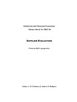
Fig. 2 The shaded region marks the ambit set A from (18) defined by (19) where the parameters
are chosen to be Tlarge = 1, Tsmall = 0.1 and θ = 5

where Tlarge > 0. For Tlarge > Tsmall > 0 and θ > 0, the function f is defined as
f (t) =

1 − (t/Tlarge )θ
1 + (t/Tsmall )θ

1/θ

, 0 ≤ t ≤ Tlarge .

(19)

The shape of the ambit set is chosen so that the scaling behaviour (15) of the correlators is reproduced. The exact values of the scaling exponents are determined from
the distribution of the Lévy seed of the Lévy basis. The two parameters Tsmall and
Tlarge determine the size of the small and large scales of turbulence: in between we
have the inertial range. The final parameter θ is a tuning parameter which accounts
for the lack of perfect scaling and essentially just allows for a better fit. (Perfect
scaling is obtained in the limit θ → ∞). See Fig. 2 for an example. Furthermore,
self-scaling exponents are predicted from the shape, not location and scale, of the
one-point distribution of the energy dissipation alone.
To determine a proper distribution of the Lévy seed of L, it is in [31] shown
that the one-dimensional marginal of the logarithm of the energy dissipation is well
described by a normal inverse Gaussian distribution, i.e. log ε(t) ∼ NIG(α, β, μ, δ),

where the shape parameters α and β are the same for all datasets (independent of
the Reynolds number). Thus the shape of the distribution of the energy dissipation
is a newly discovered universal feature of turbulence. Thus we see that L should be
a normal inverse Gaussian Lévy basis whose parameters are given by the observed
distribution of log ε(t). This completely specifies the parameters of (17).


Some Recent Developments in Ambit Stochastics

13

4.2 Realised Relative Volatility/Intermittency/Energy
Dissipation
By its very nature, volatility/intermittency is a relative concept, delineating variation that is relative to a conceived, simpler model. But also in a model for volatility/intermittency in itself it is relevant to have the relative character in mind, as
will be further discussed below. We refer to this latter aspect as relative volatility/intermittency and will consider assessment of that by realised relative volatility/intermittency which is defined in terms of quadratic variation. The ultimate
purpose of the concept of relative volatility/intermittency is to assess the volatility/intermittency or energy dissipation in arbitrary subregions of a region C of spacetime relative to the total volatility/intermittency/energy dissipation in C. In the purely
temporal setting the realised relative volatility/intermittency is defined by
[Yδ ]t /[Yδ ]T

(20)

where [Yδ ]t denotes the realised quadratic variation of the process Y observed with
lag δ over a time interval [0, t]. We refer to this quantity as RRQV (for realised
relative quadratic volatility).
As mentioned in Example 1, in case g is the gamma kernel (8) with ν ∈ (1/2, 1)∪
(1, 3/2] then the BSS process (7) is not a semimartingale. In particular, if ν ∈
(1/2, 1)—the case of most interest for the study of turbulence—the realised quadratic
variation [Yδ ]t does not converge as it would if Y was a semimartingale; in fact it
diverges to infinity whereas in the semimartingale case it will generally converge to
the accumulated volatility/intermittency

σt2+ =

t
0

σs2 ds,

(21)

which is an object of key interest (in turbulence it represents the coarse-grained
energy dissipation). However the situation can be remedied by adjusting [Yδ ]t by a
factor depending on ν; in wide generality it holds that
p

cδ 2(1−ν) [Yδ ]t −→ σt2+

(22)

as δ −→ 0, with x = λ−1 22(ν−1/2) (Γ (ν) + Γ (ν + 1/2))/Γ (2ν − 1)Γ (3/2 − 1). To
apply this requires knowledge of the value of ν and in general ν must be estimated with
sufficient precision to ensure that substituting the estimate for the theoretical value of
ν in (22) will still yield convergence in probability. Under relatively mild conditions
that is possible, as discussed in [26] and the references therein. An important aspect
of formula (20) is that its use does not involve knowledge of ν as the adjustment
factor cancels out (Fig. 3).
Convergence in probability and a central limit theorem for the RRQV is established in [10]. Figure 2 illustrates its use, for two sections of the “Brookhaven” dataset,


14

O.E. Barndorff-Nielsen et al.

Fig. 3 Brookhaven turbulence data periods 18 and 25—RRQV and 95 % confidence intervals

one where the volatility effect was deemed by eye to be very small and one where
it appeared strong. (The “Brookhaven” dataset consist of 20 million one-point measurements of the longitudinal component of the wind velocity in the atmospheric
boundary layer, 35 m above ground. The measurements were performed using a
hot-wire anemometer and sampled at 5 kHz. The time series can be assumed to be
stationary. We refer to [27] for further details on the dataset; the dataset is called
no. 3 therein).

4.3 Role of Selfdecomposability
If τ is given by (12) it is automatically infinitely divisible, and selfdecomposable
provided L has that property; whereas if τ is defined by (13) it will only in exceptional
cases be infinitely divisible.
A non-trivial example of such an exceptional case is the following. The Gumbel
distribution with density
f (x) =

x −a
x −a
1
exp
− exp
b
b
b

,

(23)

where a ∈ R and b > 0 is infinitely divisible [39]. In [31] it was demonstrated that
the one-dimensional marginal distribution of the logarithm of the energy dissipation
is accurately described by a normal inverse Gaussian distribution. One may also
show (not done here) that the Gumbel distribution with b = 2 provides another fit
that is nearly as accurate as the normal inverse Gaussian. Furthermore, if X is a
Gumbel random variable with b = 2, then exp(X ) is distributed as the square of
an exponential random variable, hence also infinitely divisible by [39]. Therefore, if


Some Recent Developments in Ambit Stochastics

15

the Lévy basis L in (17) is chosen so that L(A) follows a Gumbel distribution with
b = 2, then exp(L(A(t))) will be infinitely divisible.
For a general discussion of selfdecomposable fields we refer to [13]. See also [32]
which provides a survey of when a selfdecomposable random variable can be represented as a stochastic integral, like in (12). Representations of that kind allow, in
particular, the construction of field-valued processes of OU or supOU type that may
be viewed as propagating, in time, an initial volatility/intermittency field defined on
the spatial component of space-time for a fixed time, say t = 0. Similarly, suppose
that a model has been formulated for the time-wise development of a stochastic field
at a single point in space. One may then seek to define a field on space-time such that
at every other point of space the time-wise development of the field is stochastically
the same as at the original space point and such that the field as a whole is stationary
and selfdecomposable.
Example 1 (One dimensional turbulence) Let Y denote an ambit field in the tempospatial case where the spatial dimension is 1, and assume that for a preliminary purely
temporal model X of the same turbulent phenomenon a model has been formulated
for the squared amplitude volatility component, say ω. It may then be desirable

to devise Y such that the volatility/intermittency field τ = σ 2 is stationary and
infinitely divisible, and such that for every spatial position x the law of τ (x, · ) is
identical to that formulated for the temporal setting, i.e. ω. If the temporal process
is selfdecomposable then, subject to a further weak condition (see [13]), such a field
can be constructed.
To sketch how this may proceed, recall first that the classical definition of selfdecomposability of a process X says that all the finite-dimensional marginal distributions of X should be selfdecomposable. Accordingly, due to a result by [38], for
any finite set of time points uˆ = (u 1 , . . . , u n ) the selfdecomposable vector variable
X (u)
ˆ = (X (u 1 ), . . . , X (u n )) has a representation
∞

X (u)
ˆ =

e−ξ L(dξ, u)
ˆ

0

for some n-dimensional Lévy process L( · , u),
ˆ provided only that the Lévy measure
of X (u)
ˆ has finite log-moment. We now assume this to be the case and that X is
stationary
˜
Next, for fixed u,
ˆ let { L(x,
u)
ˆ | x ∈ R}, be the n-dimensional Lévy process having
˜

the property that the law of L(1,
u)
ˆ is equal to the law of X (u).
ˆ Then the integral
X (x, u)
ˆ =

x
−∞

˜
e−ξ L(dξ,
u)
ˆ

exists and the process {X (x, u)
ˆ | x ∈ R} will be stationary—of Ornstein-Uhlenbeck
type—while for each x the law of X (x, u)
ˆ will be the same as that of X (u).
ˆ


16

O.E. Barndorff-Nielsen et al.

˜ · , u)
However, off hand the Lévy processes L(
ˆ corresponding to different sets uˆ
of time points may have no dynamic relationship to each other, while the aim is to

obtain a stationary selfdecomposable field X (x, t) such that X (x, · ) has the same
law as X for all x ∈ R. But, arguing along the lines of theorem 3.4 in [9], it is possible
˜ · , u)
to choose the representative processes L(
ˆ so that they are all defined on a single
probability space and are consistent among themselves (in analogy to Kolmogorov’s
consistency result); and that establishes the existence of the desired field X (x, t).
Moreover, X ( · , · ) is selfdecomposable, as is simple to verify.
The same result can be shown more directly using master Lévy measures and the
associated Lévy-Ito representations, cf. [13].
Example 2 Assume that X has the form
X (u) =

u
−∞

g(u − ξ ) L(dξ )

(24)

where L is a Lévy process.
It has been shown in [13] that, in this case, provided g is integrable with respect
to the Lebesgue measure, as well as to L, and if the Fourier transform of g is nonvanishing, then X , as a process, is selfdecomposable if and only if L is selfdecomposable. When that holds we may, as above, construct a selfdecomposable field X (x, t)
with X (x, · ) ∼ X ( · ) for every x ∈ R and X ( · , t) of OU type for every t ∈ R.
As an illustration, suppose that g is the gamma kernel (8) with ν ∈ (1/2, 1). Then
the Fourier transform of g is
g(ζ
ˆ ) = (1 − iζ /λ)−ν .
and hence, provided that L is such that the integral (24) exists, the field X (x, u) is
stationary and selfdecomposable, and has the OU type character described above.

5 Time Change and Universality in Turbulence
and Finance
5.1 Distributional Collapse
In [4], Barndorff-Nielsen et al. demonstrate two properties of the distributions of
increments Δ X (t) = X (t) − X (t − ) of turbulent velocities. Firstly, the increment
distributions are parsimonious, i.e., they are described well by a distribution with
few parameters, even across distinct experiments. Specifically it is shown that the


Some Recent Developments in Ambit Stochastics

17

four-parameter family of normal inverse Gaussian distributions (NIG(α, β, μ, δ))
provides excellent fits across a wide range of lags ,
Δ X ∼ NIG(α( ), β( ), μ( ), δ( )).

(25)

Secondly, the increment distributions are universal, i.e., the distributions are the same
for distinct experiments, if just the scale parameters agree,
Δ 1 X1 ∼ Δ 2 X2

if and only if

δ1 ( 1 ) = δ2 ( 2 ),

(26)

provided the original velocities (not increments) have been non-dimensionalized
by standardizing to zero mean and unit variance. Motivated by this, the notion of
stochastic equivalence class is introduced.
The line of study initiated in [4] is continued in [16], where the analysis is extended
to many more data sets, and it is observed that
Δ 1 X1 ∼ Δ 2 X2

if and only if

var(Δ 1 X 1 ) ∼ var(Δ 2 X 2 ),

(27)

which is a simpler statement than (26), since it does not involve any specific distribution. In [21], Barndorff-Nielsen et al. extend the analysis from fluid velocities in
turbulence to currency and metal returns in finance and demonstrate that (27) holds
when X i denotes the log-price, so increments are log-returns. Further corroboration of the existence of this phenomenon in finance is presented in the following
subsection.
A conclusion from the cited works is that within the context of turbulence or
finance there exists a family of distributions such that for many distinct experiments
and a wide range of lags, the corresponding increments are distributed according
to a member of this family. Moreover, this member is uniquely determined by the
variance of the increments.
Up till recently these stylised features had not been given any theoretical background. However, in [20], a class of stochastic processes is introduced that exactly
has the rescaling property in question.

5.2 A First Look at Financial Data from SP500
Motivated by the developments discussed in the previous subsection, in the following
we complement the analyses in [4, 16, 21] with 29 assets from Standard & Poor’s
500 stock market index. The following assets were selected for study: AA, AIG,
AXP, BA, BAC, C, CAT, CVX, DD, DIS, GE, GM, HD, IBM, INTC, JNJ, JPM, KO,

MCD, MMM, MRK, MSFT, PG, SPY, T, UTX, VZ, WMT, XOM. For each asset,
between 7 and 12 years of data is available. A sample time series of the log-price of
asset C is displayed in Fig. 4, where the thin vertical line marks the day 2008-01-01.