2014 applied statistical inference likelihood and bayes
Bạn đang xem bản rút gọn của tài liệu. Xem và tải ngay bản đầy đủ của tài liệu tại đây (10.56 MB, 382 trang )
Leonhard Held
Daniel Sabanés Bové
Applied
Statistical
Inference
Likelihood and Bayes
Applied Statistical Inference
Leonhard Held r Daniel Sabanés Bové
Applied
Statistical
Inference
Likelihood and Bayes
Leonhard Held
Institute of Social and Preventive Medicine
University of Zurich
Zurich, Switzerland
Daniel Sabanés Bové
Institute of Social and Preventive Medicine
University of Zurich
Zurich, Switzerland
ISBN 978-3-642-37886-7
ISBN 978-3-642-37887-4 (eBook)
DOI 10.1007/978-3-642-37887-4
Springer Heidelberg New York Dordrecht London
Library of Congress Control Number: 2013954443
Mathematics Subject Classification: 62-01, 62F10, 62F12, 62F15, 62F25, 62F40, 62P10, 65C05, 65C60
© Springer-Verlag Berlin Heidelberg 2014
This work is subject to copyright. All rights are reserved by the Publisher, whether the whole or part of
the material is concerned, specifically the rights of translation, reprinting, reuse of illustrations, recitation,
broadcasting, reproduction on microfilms or in any other physical way, and transmission or information
storage and retrieval, electronic adaptation, computer software, or by similar or dissimilar methodology
now known or hereafter developed. Exempted from this legal reservation are brief excerpts in connection
with reviews or scholarly analysis or material supplied specifically for the purpose of being entered
and executed on a computer system, for exclusive use by the purchaser of the work. Duplication of
this publication or parts thereof is permitted only under the provisions of the Copyright Law of the
Publisher’s location, in its current version, and permission for use must always be obtained from Springer.
Permissions for use may be obtained through RightsLink at the Copyright Clearance Center. Violations
are liable to prosecution under the respective Copyright Law.
The use of general descriptive names, registered names, trademarks, service marks, etc. in this publication
does not imply, even in the absence of a specific statement, that such names are exempt from the relevant
protective laws and regulations and therefore free for general use.
While the advice and information in this book are believed to be true and accurate at the date of publication, neither the authors nor the editors nor the publisher can accept any legal responsibility for any
errors or omissions that may be made. The publisher makes no warranty, express or implied, with respect
to the material contained herein.
Printed on acid-free paper
Springer is part of Springer Science+Business Media (www.springer.com)
To My Family: Ulrike, Valentina, Richard
and Lorenz
To My Wonderful Wife Katja
Preface
Statistical inference is the science of analysing and interpreting data. It provides
essential tools for processing information, summarizing the amount of knowledge
gained and quantifying the remaining uncertainty.
This book provides an introduction to the principles and concepts of the two
most commonly used methods in scientific investigations: Likelihood and Bayesian
inference. The two approaches are usually seen as competing paradigms, but we
also emphasise connections, as there are many. In particular, both approaches are
linked to the notion of a statistical model and the corresponding likelihood function,
as described in the first two chapters. We discuss frequentist inference based on
the likelihood in detail, followed by the essentials of Bayesian inference. Advanced
topics that are important in practice are model selection, prediction and numerical
computation, and these are also discussed from both perspectives.
The intended audience are graduate students of Statistics, Biostatistics, Applied
Mathematics, Biomathematics and Bioinformatics. The reader should be familiar
with elementary concepts of probability, calculus, matrix algebra and numerical
analysis, as summarised in detailed Appendices A–C. Several applications, taken
from the area of biomedical research, are described in the Introduction and serve
as examples throughout the book. We hope that the R code provided will make it
easy for the reader to apply the methods discussed to her own statistical problem.
Each chapter finishes with exercises, which can be used to deepen the knowledge
obtained.
This textbook is based on a series of lectures and exercises that we gave at the
University of Zurich for Master students in Statistics and Biostatistics. It is a substantial extension of the German book “Methoden der statistischen Inferenz: Likelihood und Bayes”, published by Spektrum Akademischer Verlag (Held 2008). Many
people have helped in various ways. We like to thank Eva and Reinhard Furrer,
Torsten Hothorn, Andrea Riebler, Malgorzata Roos, Kaspar Rufibach and all the
others that we forgot in this list. Last but not least, we are grateful to Niels Peter
Thomas, Alice Blanck and Ulrike Stricker-Komba from Springer-Verlag Heidelberg
for their continuing support and enthusiasm.
Zurich, Switzerland
June 2013
Leonhard Held, Daniel Sabanés Bové
vii
Contents
1
Introduction . . . . . . . . . . . . . . . . . . . . . . . . . . . . .
1.1 Examples . . . . . . . . . . . . . . . . . . . . . . . . . . . .
1.1.1 Inference for a Proportion . . . . . . . . . . . . . . .
1.1.2 Comparison of Proportions . . . . . . . . . . . . . .
1.1.3 The Capture–Recapture Method . . . . . . . . . . . .
1.1.4 Hardy–Weinberg Equilibrium . . . . . . . . . . . . .
1.1.5 Estimation of Diagnostic Tests Characteristics . . . .
1.1.6 Quantifying Disease Risk from Cancer Registry Data
1.1.7 Predicting Blood Alcohol Concentration . . . . . . .
1.1.8 Analysis of Survival Times . . . . . . . . . . . . . .
1.2 Statistical Models . . . . . . . . . . . . . . . . . . . . . . .
1.3 Contents and Notation of the Book . . . . . . . . . . . . . .
1.4 References . . . . . . . . . . . . . . . . . . . . . . . . . . .
.
.
.
.
.
.
.
.
.
.
.
.
.
.
.
.
.
.
.
.
.
.
.
.
.
.
1
2
2
2
4
4
5
6
8
8
9
11
11
2
Likelihood . . . . . . . . . . . . . . . . . . . . . . . . . . . . . . .
2.1 Likelihood and Log-Likelihood Function . . . . . . . . . . . .
2.1.1 Maximum Likelihood Estimate . . . . . . . . . . . . .
2.1.2 Relative Likelihood . . . . . . . . . . . . . . . . . . .
2.1.3 Invariance of the Likelihood . . . . . . . . . . . . . . .
2.1.4 Generalised Likelihood . . . . . . . . . . . . . . . . .
2.2 Score Function and Fisher Information . . . . . . . . . . . . .
2.3 Numerical Computation of the Maximum Likelihood Estimate
2.3.1 Numerical Optimisation . . . . . . . . . . . . . . . . .
2.3.2 The EM Algorithm . . . . . . . . . . . . . . . . . . .
2.4 Quadratic Approximation of the Log-Likelihood Function . . .
2.5 Sufficiency . . . . . . . . . . . . . . . . . . . . . . . . . . . .
2.5.1 Minimal Sufficiency . . . . . . . . . . . . . . . . . . .
2.5.2 The Likelihood Principle . . . . . . . . . . . . . . . .
2.6 Exercises . . . . . . . . . . . . . . . . . . . . . . . . . . . . .
2.7 Bibliographic Notes . . . . . . . . . . . . . . . . . . . . . . .
.
.
.
.
.
.
.
.
.
.
.
.
.
.
.
.
13
13
14
22
23
26
27
31
31
34
37
40
45
47
48
50
3
Elements of Frequentist Inference . . . . .
3.1 Unbiasedness and Consistency . . . .
3.2 Standard Error and Confidence Interval
3.2.1 Standard Error . . . . . . . . .
.
.
.
.
51
51
55
56
.
.
.
.
.
.
.
.
.
.
.
.
.
.
.
.
.
.
.
.
.
.
.
.
.
.
.
.
.
.
.
.
.
.
.
.
.
.
.
.
.
.
.
.
.
.
.
.
.
.
.
.
ix
x
Contents
3.2.2 Confidence Interval . . .
3.2.3 Pivots . . . . . . . . . .
3.2.4 The Delta Method . . . .
3.2.5 The Bootstrap . . . . . .
3.3 Significance Tests and P -Values .
3.4 Exercises . . . . . . . . . . . . .
3.5 References . . . . . . . . . . . .
.
.
.
.
.
.
.
.
.
.
.
.
.
.
.
.
.
.
.
.
.
.
.
.
.
.
.
.
56
59
63
65
70
75
78
4
Frequentist Properties of the Likelihood . . . . . . . . . . . .
4.1 The Expected Fisher Information and the Score Statistic . .
4.1.1 The Expected Fisher Information . . . . . . . . . .
4.1.2 Properties of the Expected Fisher Information . . .
4.1.3 The Score Statistic . . . . . . . . . . . . . . . . . .
4.1.4 The Score Test . . . . . . . . . . . . . . . . . . . .
4.1.5 Score Confidence Intervals . . . . . . . . . . . . .
4.2 The Distribution of the ML Estimator and the Wald Statistic
4.2.1 Cramér–Rao Lower Bound . . . . . . . . . . . . .
4.2.2 Consistency of the ML Estimator . . . . . . . . . .
4.2.3 The Distribution of the ML Estimator . . . . . . . .
4.2.4 The Wald Statistic . . . . . . . . . . . . . . . . . .
4.3 Variance Stabilising Transformations . . . . . . . . . . . .
4.4 The Likelihood Ratio Statistic . . . . . . . . . . . . . . . .
4.4.1 The Likelihood Ratio Test . . . . . . . . . . . . . .
4.4.2 Likelihood Ratio Confidence Intervals . . . . . . .
4.5 The p ∗ Formula . . . . . . . . . . . . . . . . . . . . . . .
4.6 A Comparison of Likelihood-Based Confidence Intervals .
4.7 Exercises . . . . . . . . . . . . . . . . . . . . . . . . . . .
4.8 References . . . . . . . . . . . . . . . . . . . . . . . . . .
.
.
.
.
.
.
.
.
.
.
.
.
.
.
.
.
.
.
.
.
.
.
.
.
.
.
.
.
.
.
.
.
.
.
.
.
.
.
.
.
.
.
.
.
.
.
.
.
.
.
.
.
.
.
.
.
.
.
.
.
79
80
81
84
87
89
91
94
95
96
97
99
101
105
106
106
112
113
119
122
5
Likelihood Inference in Multiparameter Models . . . . . .
5.1 Score Vector and Fisher Information Matrix . . . . . .
5.2 Standard Error and Wald Confidence Interval . . . . . .
5.3 Profile Likelihood . . . . . . . . . . . . . . . . . . . .
5.4 Frequentist Properties of the Multiparameter Likelihood
5.4.1 The Score Statistic . . . . . . . . . . . . . . . .
5.4.2 The Wald Statistic . . . . . . . . . . . . . . . .
5.4.3 The Multivariate Delta Method . . . . . . . . .
5.4.4 The Likelihood Ratio Statistic . . . . . . . . . .
5.5 The Generalised Likelihood Ratio Statistic . . . . . . .
5.6 Conditional Likelihood . . . . . . . . . . . . . . . . .
5.7 Exercises . . . . . . . . . . . . . . . . . . . . . . . . .
5.8 References . . . . . . . . . . . . . . . . . . . . . . . .
.
.
.
.
.
.
.
.
.
.
.
.
.
.
.
.
.
.
.
.
.
.
.
.
.
.
.
.
.
.
.
.
.
.
.
.
.
.
.
.
.
.
.
.
.
.
.
.
.
.
.
.
.
.
.
.
.
.
.
.
.
.
.
.
.
123
124
128
130
143
144
145
146
146
148
153
155
165
6
Bayesian Inference . . . . . . . . .
6.1 Bayes’ Theorem . . . . . . . .
6.2 Posterior Distribution . . . . .
6.3 Choice of the Prior Distribution
.
.
.
.
.
.
.
.
.
.
.
.
.
.
.
.
.
.
.
.
167
168
170
179
.
.
.
.
.
.
.
.
.
.
.
.
.
.
.
.
.
.
.
.
.
.
.
.
.
.
.
.
.
.
.
.
.
.
.
.
.
.
.
.
.
.
.
.
.
.
.
.
.
.
.
.
.
.
.
.
.
.
.
.
.
.
.
.
.
.
.
.
.
.
.
.
.
.
.
.
.
.
.
.
.
.
.
.
.
.
.
.
.
.
.
.
.
.
.
.
.
.
.
.
.
.
.
.
.
.
.
.
.
.
.
.
.
.
.
.
.
.
.
.
.
.
.
.
.
.
.
.
.
.
.
.
.
.
.
.
.
.
.
.
.
.
.
Contents
6.4
6.5
6.6
6.7
6.8
6.9
xi
6.3.1 Conjugate Prior Distributions . . . . . . . . . . . . . .
6.3.2 Improper Prior Distributions . . . . . . . . . . . . . . .
6.3.3 Jeffreys’ Prior Distributions . . . . . . . . . . . . . . .
Properties of Bayesian Point and Interval Estimates . . . . . .
6.4.1 Loss Function and Bayes Estimates . . . . . . . . . . .
6.4.2 Compatible and Invariant Bayes Estimates . . . . . . .
Bayesian Inference in Multiparameter Models . . . . . . . . .
6.5.1 Conjugate Prior Distributions . . . . . . . . . . . . . .
6.5.2 Jeffreys’ and Reference Prior Distributions . . . . . . .
6.5.3 Elimination of Nuisance Parameters . . . . . . . . . .
6.5.4 Compatibility of Uni- and Multivariate Point Estimates
Some Results from Bayesian Asymptotics . . . . . . . . . . .
6.6.1 Discrete Asymptotics . . . . . . . . . . . . . . . . . .
6.6.2 Continuous Asymptotics . . . . . . . . . . . . . . . . .
Empirical Bayes Methods . . . . . . . . . . . . . . . . . . . .
Exercises . . . . . . . . . . . . . . . . . . . . . . . . . . . . .
References . . . . . . . . . . . . . . . . . . . . . . . . . . . .
.
.
.
.
.
.
.
.
.
.
.
.
.
.
.
.
.
.
.
.
.
.
.
.
.
.
.
.
.
.
.
.
.
.
.
.
.
.
.
.
.
.
.
.
.
.
.
.
.
.
.
.
.
.
.
.
.
.
.
.
.
.
.
.
.
.
.
.
.
.
.
.
.
.
.
.
.
.
.
.
.
.
.
.
.
.
.
.
.
179
183
185
192
192
195
196
196
198
200
204
204
205
206
209
214
219
7
Model Selection . . . . . . . . . . . . . . . . . . .
7.1 Likelihood-Based Model Selection . . . . . .
7.1.1 Akaike’s Information Criterion . . . .
7.1.2 Cross Validation and AIC . . . . . . .
7.1.3 Bayesian Information Criterion . . . .
7.2 Bayesian Model Selection . . . . . . . . . . .
7.2.1 Marginal Likelihood and Bayes Factor
7.2.2 Marginal Likelihood and BIC . . . . .
7.2.3 Deviance Information Criterion . . . .
7.2.4 Model Averaging . . . . . . . . . . .
7.3 Exercises . . . . . . . . . . . . . . . . . . . .
7.4 References . . . . . . . . . . . . . . . . . . .
.
.
.
.
.
.
.
.
.
.
.
.
.
.
.
.
.
.
.
.
.
.
.
.
.
.
.
.
.
.
.
.
.
.
.
.
.
.
.
.
.
.
.
.
.
.
.
.
221
224
224
227
230
231
232
236
239
240
243
245
8
Numerical Methods for Bayesian Inference . . . . . . . . . .
8.1 Standard Numerical Techniques . . . . . . . . . . . . . . .
8.2 Laplace Approximation . . . . . . . . . . . . . . . . . . .
8.3 Monte Carlo Methods . . . . . . . . . . . . . . . . . . . .
8.3.1 Monte Carlo Integration . . . . . . . . . . . . . . .
8.3.2 Importance Sampling . . . . . . . . . . . . . . . .
8.3.3 Rejection Sampling . . . . . . . . . . . . . . . . .
8.4 Markov Chain Monte Carlo . . . . . . . . . . . . . . . . .
8.5 Numerical Calculation of the Marginal Likelihood . . . . .
8.5.1 Calculation Through Numerical Integration . . . . .
8.5.2 Monte Carlo Estimation of the Marginal Likelihood
8.6 Exercises . . . . . . . . . . . . . . . . . . . . . . . . . . .
8.7 References . . . . . . . . . . . . . . . . . . . . . . . . . .
.
.
.
.
.
.
.
.
.
.
.
.
.
.
.
.
.
.
.
.
.
.
.
.
.
.
.
.
.
.
.
.
.
.
.
.
.
.
.
247
248
253
258
258
265
267
269
280
280
282
286
289
xii
9
Contents
Prediction . . . . . . . . . . . . . . . . . . . . . . . . . . . . .
9.1 Plug-in Prediction . . . . . . . . . . . . . . . . . . . . . .
9.2 Likelihood Prediction . . . . . . . . . . . . . . . . . . . .
9.2.1 Predictive Likelihood . . . . . . . . . . . . . . . .
9.2.2 Bootstrap Prediction . . . . . . . . . . . . . . . . .
9.3 Bayesian Prediction . . . . . . . . . . . . . . . . . . . . .
9.3.1 Posterior Predictive Distribution . . . . . . . . . . .
9.3.2 Computation of the Posterior Predictive Distribution
9.3.3 Model Averaging . . . . . . . . . . . . . . . . . .
9.4 Assessment of Predictions . . . . . . . . . . . . . . . . . .
9.4.1 Discrimination and Calibration . . . . . . . . . . .
9.4.2 Scoring Rules . . . . . . . . . . . . . . . . . . . .
9.5 Exercises . . . . . . . . . . . . . . . . . . . . . . . . . . .
9.6 References . . . . . . . . . . . . . . . . . . . . . . . . . .
.
.
.
.
.
.
.
.
.
.
.
.
.
.
.
.
.
.
.
.
.
.
.
.
.
.
.
.
.
.
.
.
.
.
.
.
.
.
.
.
.
.
291
292
292
293
295
299
299
303
305
306
307
311
315
316
Appendix A Probabilities, Random Variables and Distributions . . . .
A.1 Events and Probabilities . . . . . . . . . . . . . . . . . . . . . .
A.1.1 Conditional Probabilities and Independence . . . . . . .
A.1.2 Bayes’ Theorem . . . . . . . . . . . . . . . . . . . . . .
A.2 Random Variables . . . . . . . . . . . . . . . . . . . . . . . . .
A.2.1 Discrete Random Variables . . . . . . . . . . . . . . . .
A.2.2 Continuous Random Variables . . . . . . . . . . . . . .
A.2.3 The Change-of-Variables Formula . . . . . . . . . . . .
A.2.4 Multivariate Normal Distributions . . . . . . . . . . . . .
A.3 Expectation, Variance and Covariance . . . . . . . . . . . . . . .
A.3.1 Expectation . . . . . . . . . . . . . . . . . . . . . . . .
A.3.2 Variance . . . . . . . . . . . . . . . . . . . . . . . . . .
A.3.3 Moments . . . . . . . . . . . . . . . . . . . . . . . . . .
A.3.4 Conditional Expectation and Variance . . . . . . . . . . .
A.3.5 Covariance . . . . . . . . . . . . . . . . . . . . . . . . .
A.3.6 Correlation . . . . . . . . . . . . . . . . . . . . . . . . .
A.3.7 Jensen’s Inequality . . . . . . . . . . . . . . . . . . . . .
A.3.8 Kullback–Leibler Discrepancy and Information Inequality
A.4 Convergence of Random Variables . . . . . . . . . . . . . . . .
A.4.1 Modes of Convergence . . . . . . . . . . . . . . . . . .
A.4.2 Continuous Mapping and Slutsky’s Theorem . . . . . . .
A.4.3 Law of Large Numbers . . . . . . . . . . . . . . . . . .
A.4.4 Central Limit Theorem . . . . . . . . . . . . . . . . . .
A.4.5 Delta Method . . . . . . . . . . . . . . . . . . . . . . .
A.5 Probability Distributions . . . . . . . . . . . . . . . . . . . . . .
A.5.1 Univariate Discrete Distributions . . . . . . . . . . . . .
A.5.2 Univariate Continuous Distributions . . . . . . . . . . .
A.5.3 Multivariate Distributions . . . . . . . . . . . . . . . . .
317
318
318
319
319
319
320
321
323
324
324
325
325
325
326
327
328
329
329
329
330
330
331
331
332
333
335
339
Contents
xiii
Appendix B Some Results from Matrix Algebra and Calculus
B.1 Some Matrix Algebra . . . . . . . . . . . . . . . . . .
B.1.1 Trace, Determinant and Inverse . . . . . . . . .
B.1.2 Cholesky Decomposition . . . . . . . . . . . .
B.1.3 Inversion of Block Matrices . . . . . . . . . . .
B.1.4 Sherman–Morrison Formula . . . . . . . . . . .
B.1.5 Combining Quadratic Forms . . . . . . . . . .
B.2 Some Results from Mathematical Calculus . . . . . . .
B.2.1 The Gamma and Beta Functions . . . . . . . . .
B.2.2 Multivariate Derivatives . . . . . . . . . . . . .
B.2.3 Taylor Approximation . . . . . . . . . . . . . .
B.2.4 Leibniz Integral Rule . . . . . . . . . . . . . .
B.2.5 Lagrange Multipliers . . . . . . . . . . . . . .
B.2.6 Landau Notation . . . . . . . . . . . . . . . . .
.
.
.
.
.
.
.
.
.
.
.
.
.
.
.
.
.
.
.
.
.
.
.
.
.
.
.
.
.
.
.
.
.
.
.
.
.
.
.
.
.
.
.
.
.
.
.
.
.
.
.
.
.
.
.
.
.
.
.
.
.
.
.
.
.
.
.
.
.
.
341
341
341
343
344
345
345
345
345
346
347
348
348
349
Appendix C Some Numerical Techniques . . . .
C.1 Optimisation and Root Finding Algorithms
C.1.1 Motivation . . . . . . . . . . . . .
C.1.2 Bisection Method . . . . . . . . .
C.1.3 Newton–Raphson Method . . . . .
C.1.4 Secant Method . . . . . . . . . . .
C.2 Integration . . . . . . . . . . . . . . . . .
C.2.1 Newton–Cotes Formulas . . . . . .
C.2.2 Laplace Approximation . . . . . .
.
.
.
.
.
.
.
.
.
.
.
.
.
.
.
.
.
.
.
.
.
.
.
.
.
.
.
.
.
.
.
.
.
.
.
.
.
.
.
.
.
.
.
.
.
351
351
351
352
354
357
358
358
361
Notation . . . . . . . . . . . . . . . . . . . . . . . . . . . . . . . . . . . .
363
References . . . . . . . . . . . . . . . . . . . . . . . . . . . . . . . . . .
367
Index . . . . . . . . . . . . . . . . . . . . . . . . . . . . . . . . . . . . .
371
.
.
.
.
.
.
.
.
.
.
.
.
.
.
.
.
.
.
.
.
.
.
.
.
.
.
.
.
.
.
.
.
.
.
.
.
.
.
.
.
.
.
.
.
.
.
.
.
.
.
.
.
.
.
.
.
.
.
.
.
.
.
.
1
Introduction
Contents
1.1
1.2
1.3
1.4
Examples . . . . . . . . . . . . . . . . . . . . . . . . . . .
1.1.1 Inference for a Proportion . . . . . . . . . . . . . .
1.1.2 Comparison of Proportions . . . . . . . . . . . . . .
1.1.3 The Capture–Recapture Method . . . . . . . . . . .
1.1.4 Hardy–Weinberg Equilibrium . . . . . . . . . . . .
1.1.5 Estimation of Diagnostic Tests Characteristics . . . .
1.1.6 Quantifying Disease Risk from Cancer Registry Data
1.1.7 Predicting Blood Alcohol Concentration . . . . . . .
1.1.8 Analysis of Survival Times . . . . . . . . . . . . . .
Statistical Models . . . . . . . . . . . . . . . . . . . . . . .
Contents and Notation of the Book . . . . . . . . . . . . . .
References . . . . . . . . . . . . . . . . . . . . . . . . . .
.
.
.
.
.
.
.
.
.
.
.
.
.
.
.
.
.
.
.
.
.
.
.
.
.
.
.
.
.
.
.
.
.
.
.
.
.
.
.
.
.
.
.
.
.
.
.
.
.
.
.
.
.
.
.
.
.
.
.
.
.
.
.
.
.
.
.
.
.
.
.
.
.
.
.
.
.
.
.
.
.
.
.
.
.
.
.
.
.
.
.
.
.
.
.
.
.
.
.
.
.
.
.
.
.
.
.
.
.
.
.
.
.
.
.
.
.
.
.
.
.
.
.
.
.
.
.
.
.
.
.
.
.
.
.
.
.
.
.
.
.
.
.
.
2
2
2
4
4
5
6
8
8
9
11
11
Statistics is a discipline with different branches. This book describes two central approaches to statistical inference, likelihood inference and Bayesian inference. Both
concepts have in common that they use statistical models depending on unknown
parameters to be estimated from the data. Moreover, both are constructive, i.e. provide precise procedures for obtaining the required results. A central role is played
by the likelihood function, which is determined by the choice of a statistical model.
While a likelihood approach bases inference only on the likelihood, the Bayesian
approach combines the likelihood with prior information. Also hybrid approaches
do exist.
What do we want to learn from data using statistical inference? We can distinguish three major goals. Of central importance is to estimate the unknown parameters of a statistical model. This is the so-called estimation problem. However, how
do we know that the chosen model is correct? We may have a number of statistical
models and want to identify the one that describes the data best. This is the so-called
model selection problem. And finally, we may want to predict future observations
based on the observed ones. This is the prediction problem.
L. Held, D. Sabanés Bové, Applied Statistical Inference,
DOI 10.1007/978-3-642-37887-4_1, © Springer-Verlag Berlin Heidelberg 2014
1
2
1.1
1 Introduction
Examples
Several examples will be considered throughout this book, many of them more than
once viewed from different perspectives or tackled with different techniques. We
will now give a brief overview.
1.1.1
Inference for a Proportion
One of the oldest statistical problems is the estimation of a probability based on an
observed proportion. The underlying statistical model assumes that a certain event
of interest occurs with probability π , say. For example, a possible event is the occurrence of a specific genetic defect, for example Klinefelter’s syndrome, among
male newborns in a population of interest. Suppose now that n male newborns are
screened for that genetic defect and x ∈ {0, 1, . . . , n} newborns do have it, i.e. n − x
newborns do not have this defect. The statistical task is now to estimate from this
sample the underlying probability π for Klinefelter’s syndrome for a randomly selected male newborn in that population.
The statistical model described above is called binomial. In that model, n is fixed,
and x is a the realisation of a binomial random variable. However, the binomial
model is not the only possible one: A proportion may in fact be the result of a
different sampling scheme with the role of x and n being reversed. The resulting
negative binomial model fixes x and checks all incoming newborns for the genetic
defect considered until x newborns with the genetic defects are observed. Thus,
in this model the total number n of newborns screened is random and follows a
negative binomial distribution. See Appendix A.5.1 for properties of the binomial
and negative binomial distributions. The observed proportion x/n of newborns with
Klinefelter’s syndrome is an estimate of the probability π in both cases, but the statistical model underlying the sampling process may still affect our inference for π .
We will return to this issue in Sect. 2.5.2.
Probabilities are often transformed to odds, where the odds ω = π/(1 − π) are
defined as the ratio of the probability π of the event considered and the probability
1 − π of the complementary event. For example, a probability π = 0.5 corresponds
to 1 to 1 odds (ω = 1), while odds of 9 to 1 (ω = 9) are equivalent to a probability of
π = 0.9. The corresponding estimate of ω is given by the empirical odds x/(n − x).
It is easy to show that any odds ω can be back-transformed to the corresponding
probability π via π = ω/(1 + ω).
1.1.2
Comparison of Proportions
Closely related to inference for a proportion is the comparison of two proportions.
For example, a clinical study may be conducted to compare the risk of a certain
disease in a treatment and a control group. We now have two unknown risk probabilities π1 and π2 , with observations x1 and x2 and samples sizes n1 and n2 in
1.1
Examples
Table 1.1 Incidence of
preeclampsia (observed
proportion) in nine
randomised
placebo-controlled clinical
trials of diuretics. Empirical
odds ratios (OR) are also
given. The studies are
labelled with the name of the
principal author
3
Trial
Treatment
Weseley
11 %
(14/131)
10 %
(14/136)
1.04
Flowers
5%
(21/385)
13 %
(17/134)
0.40
Menzies
25 %
(14/57)
50 %
(24/48)
0.33
Fallis
16 %
(6/38)
45 %
(18/40)
0.23
5%
(35/760)
0.25
Cuadros
1%
(12/1011)
Control
OR
Landesman 10 %
(138/1370) 13 %
(175/1336)
0.74
Krans
3%
(15/506)
4%
(20/524)
0.77
Tervila
6%
(6/108)
2%
(2/103)
2.97
42 %
(65/153)
39 %
(40/102)
1.14
Campbell
the two groups. Different measures are now employed to compare the two groups,
among which the risk difference π1 − π2 and the risk ratio π1 /π2 are the most
common ones. The odds ratio
ω1 π1 /(1 − π1 )
=
,
ω2 π2 /(1 − π2 )
the ratio of the odds ω1 and ω2 , is also often used. Note that if the risk in the two
groups is equal, i.e. π1 = π2 , then the risk difference is zero, while both the risk ratio
and the odds ratio is one. Statistical methods can now be employed to investigate if
the simpler model with one parameter π = π1 = π2 can be preferred over the more
complex one with different risk parameters π1 and π2 . Such questions may also be
of interest if more than two groups are considered.
A controlled clinical trial compares the effect of a certain treatment with a control group, where typically either a standard treatment or a placebo treatment is
provided. Several randomised controlled clinical trials have investigated the use of
diuretics in pregnancy to prevent preeclampsia. Preeclampsia is a medical condition
characterised by high blood pressure and significant amounts of protein in the urine
of a pregnant woman. It is a very dangerous complication of a pregnancy and may
affect both the mother and fetus. In each trial women were randomly assigned to one
of the two treatment groups. Randomisation is used to exclude possible subjective
influence from the examiner and to ensure equal distribution of relevant risk factors
in the two groups.
The results of nine such studies are reported in Table 1.1. For each trial the observed proportions xi /ni in the treatment and placebo control group (i = 1, 2) are
given, as well as the corresponding empirical odds ratio
x1 /(n1 − x1 )
.
x2 /(n2 − x2 )
One can see substantial variation of the empirical odds ratios reported in Table 1.1.
This raises the question if this variation is only statistical in nature or if there is
evidence for additional heterogeneity between the studies. In the latter case the true
4
1 Introduction
treatment effect differs from trial to trial due to different inclusion criteria, different
underlying populations, or other reasons. Such questions are addressed in a metaanalysis, a combined analysis of results from different studies.
1.1.3
The Capture–Recapture Method
The capture–recapture method aims to estimate the size of a population of individuals, say the number N of fish in a lake. To do so, a sample of M fishes is drawn
from the lake, with all the fish marked and then thrown back into the lake. After a
sufficient time, a second sample of size n is taken, and the number x of marked fish
in that sample is recorded.
The goal is now to infer N from M, n and x. An ad-hoc estimate can be obtained by equating the proportion of marked fish in the lake with the corresponding
proportion in the sample:
x
M
≈ .
N
n
This leads to the estimate Nˆ ≈ M · n/x for the number N of fish in the lake. As we
will see in Example 2.2, there is a rigorous theoretical basis for this estimate. However, the estimate Nˆ has an obvious deficiency for x = 0, where Nˆ is infinite. Other
estimates without this deficiency are available. Appropriate statistical techniques
will enable us to quantify the uncertainty associated with the different estimates
of N .
1.1.4
Hardy–Weinberg Equilibrium
The Hardy–Weinberg equilibrium (after Godfrey H. Hardy, 1879–1944, and Wilhelm Weinberg, 1862–1937) plays a central in population genetics. Consider a population of diploid, sexually reproducing individuals and a specific locus on a chromosome with alleles A and a. If the allele frequencies of A and a in the population
are υ and 1 − υ, then the expected genotype frequencies of AA, Aa and aa are
π1 = υ 2 ,
π2 = 2υ(1 − υ) and π3 = (1 − υ)2 .
(1.1)
The Hardy–Weinberg equilibrium implies that the allele frequency υ determines the
expected frequencies of the genotypes. If a population is not in Hardy–Weinberg
equilibrium at a specific locus, then two parameters π1 and π2 are necessary to describe the distribution. The de Finetti diagram shown in Fig. 1.1 is a useful graphical
visualization of Hardy–Weinberg equilibrium.
It is often of interest to investigate whether a certain population is in Hardy–
Weinberg equilibrium at a particular locus. For example, a random sample of
n = 747 individuals has been taken in a study of MN blood group frequencies in
Iceland. The MN blood group in humans is under the control of a pair of alleles,
1.1
Examples
5
Fig. 1.1 The de Finetti diagram, named after the Italian statistician Bruno de Finetti (1906–1985),
displays the expected relative genotype frequencies Pr(AA) = π1 , Pr(aa) = π3 and Pr(Aa) = π2
in a bi-allelic, diploid population as the length of the perpendiculars a, b and c from the inner
point F to the sides of a equilateral triangle. The ratio of the straight length aa, Q to the side
length aa, AA is the relative allele frequency υ of A. Hardy–Weinberg equilibrium is represented
by all points on the parabola 2υ(1 − υ). For example, the point G represents such a population
with υ = 0.5, whereas population F has substantially less heterozygous Aa than expected under
Hardy–Weinberg equilibrium
M and N. Most people in the Eskimo population are MM, while other populations
tend to possess the opposite genotype NN. In the sample from Iceland, the frequencies of the underlying genotypes MM, MN and NN turned out to be x1 = 233,
x2 = 385 and x3 = 129. If we assume that the population is in Hardy–Weinberg
equilibrium, then the statistical task is to estimate the unknown allele frequency υ
from these data. Statistical methods can also address the question if the equilibrium
assumption is supported by the data or not. This is a model selection problem, which
can be addressed with a significance test or other techniques.
1.1.5
Estimation of Diagnostic Tests Characteristics
Screening of individuals is a popular public health approach to detect diseases in
an early and hopefully curable stage. In order to screen a large population, it is
imperative to use a fairly cheap diagnostic test, which typically makes errors in the
disease classification of individuals. A useful diagnostic test will have high
sensitivity = Pr(positive test | subject is diseased) and
specificity = Pr(negative test | subject is healthy).
6
1 Introduction
Table 1.2 Distribution of the number of positive test results among six consecutive screening tests
of 196 colon cancer cases
Number k of positive tests
0
1
2
3
4
5
6
Frequency Zk
?
37
22
25
29
34
49
Here Pr(A | B) denotes the conditional probability of an event A, given the information B. The first line thus reads “the sensitivity is the conditional probability of
a positive test, given the fact that the subject is diseased”; see Appendix A.1.1 for
more details on conditional probabilities. Thus, high values for the sensitivity and
specificity mean that classification of diseased and non-diseased individuals is correct with high probability. The sensitivity is also known as the true positive fraction
whereas specificity is called the true negative fraction.
Screening examinations are particularly useful if the disease considered can be
treated better in an earlier stage than in a later stage. For example, a diagnostic
study in Australia involved 38 000 individuals, which have been screened for the
presence of colon cancer repeatedly on six consecutive days with a simple diagnostic
test. 3000 individuals had at least one positive test result, which was subsequently
verified with a coloscopy. 196 cancer cases were eventually identified, and Table 1.2
reports the frequency of positive test results among those. Note that the number Z0
of cancer patients that have never been positively tested is unavailable by design.
The closely related false negative fraction
Pr(negative test | subject is diseased),
which is 1 − sensitivity, is often of central public health interest. Statistical methods
can be used to estimate this quantity and the number of undetected cancer cases Z0 .
Similarly, the false positive fraction
Pr(positive test | subject is healthy)
is 1 − specificity.
1.1.6
Quantifying Disease Risk from Cancer Registry Data
Cancer registries collect incidence and mortality data on different cancer locations.
For example, data on the incidence of lip cancer in Scotland have been collected
between 1975 and 1980. The raw counts of cancer cases in 56 administrative districts of Scotland will vary a lot due to heterogeneity in the underlying population counts. Other possible reasons for variation include different age distributions or heterogeneity in underlying risk factors for lip cancer in the different districts.
A common approach to adjust for age heterogeneity is to calculate the expected
number of cases using age standardisation. The standardised incidence ratio (SIR)
of observed to expected number of cases is then often used to visually display ge-
1.1
Examples
7
Fig. 1.2 The geographical
distribution of standardised
incidence ratios (SIRs) of lip
cancer in Scotland,
1975–1980. Note that some
SIRs are below or above the
interval [0.25, 4] and are
marked white and black,
respectively
Fig. 1.3 Plot of the
standardised incidence ratios
(SIR) versus the expected
number of lip cancer cases.
Both variables are shown on a
square-root scale to improve
visibility. The horizontal line
SIR = 1 represents equal
observed and expected cases
ographical variation in disease risk. If the SIR is equal to 1, then the observed incidence is as expected. Figure 1.2 maps the corresponding SIRs for lip cancer in
Scotland.
However, SIRs are unreliable indicators of disease incidence, in particular if the
disease is rare. For example, a small district may have zero observed cases just by
chance such that the SIR will be exactly zero. In Fig. 1.3, which plots the SIRs
versus the number of expected cases, we can identify two such districts. More generally, the statistical variation of the SIRs will depend on the population counts, so
more extreme SIRs will tend to occur in less populated areas, even if the underlying
disease risk does not vary from district to district. Indeed, we can see from Fig. 1.3
8
1 Introduction
Table 1.3 Mean and
Gender
standard deviation of the
transformation factor
TF = BAC/BrAC for females Female
and males
Male
Total
Number of
volunteers
Transformation factor
Mean
Standard deviation
33
2318.5
220.1
152
2477.5
232.5
185
2449.2
237.8
that the variation of the SIRs increases with decreasing number of expected cases.
Statistical methods can be employed to obtain more reliable estimates of disease
risk. In addition, we can also investigate the question if there is evidence for heterogeneity of the underlying disease risk at all. If this is the case, then another question
is whether the variation in disease risk is spatially structured or not.
1.1.7
Predicting Blood Alcohol Concentration
In many countries it is not allowed to drive a car with a blood alcohol concentration (BAC) above a certain threshold. For example, in Switzerland this threshold
is 0.5 mg/g = 0.5 ❤. However, usually only a measurement of the breath alcohol concentration (BrAC) is taken from a suspicious driver in the first instance. It
is therefore important to accurately predict the BAC measurement from the BrAC
measurement. Usually this is done by multiplication of the BrAC measurement with
a transformation factor TF. Ideally this transformation should be accompanied with
a prediction interval to acknowledge the uncertainty of the BAC prediction.
In Switzerland, currently TF0 = 2000 is used in practise. As some experts consider this too low, a study was conducted at the Forensic Institute of the University
of Zurich in the period 2003–2004. For n = 185 volunteers, both BrAC and BAC
were measured after consuming various amounts of alcoholic beverages of personal
choice. Mean and standard deviation of the ratio TF = BAC/BrAC are shown in
Table 1.3. One of the central questions of the study was if the currently used factor
of TF0 = 2000 needs to be adjusted. Moreover, it is of interest if the empirical difference between male and female volunteers provides evidence of a true difference
between genders.
1.1.8
Analysis of Survival Times
A randomised placebo-controlled trial of Azathioprine for primary biliary cirrhosis
(PBC) was designed with patient survival as primary outcome. PBC is a chronic and
eventually fatal liver disease, which affects mostly women. Table 1.4 gives the survival times (in days) of the 94 patients, which have been treated with Azathioprine.
The reported survival time is censored for 47 (50 %) of the patients. A censored
survival time does not represent the time of death but the last time point when the
patient was still known to be alive. It is not known whether, and if so when, a woman
1.2
Statistical Models
9
Table 1.4 Survival times of 94 patients under Azathioprine treatment in days. Censored observations are marked with a plus sign
8+
9
38
96
144
167
177
191+
193
201
425
464
498+
500
207
251
287+
335+
379+
421
574+
582+
586
616
630
636
647
651+
688
743
754
769+
797
799+
804
828+
904+
932+
947
962+
974
1113+
1219
1247
1260
1268
1292+
1408
1436+
1499
1500
1522
1552
1554
1555+
1626+
1649+
1942
1975
1982+
1998+
2024+
2058+
2063+
2101+
2114+
2148
2209
2254+
2338+
2384+
2387+
2415+
2426
2436+
2470
2495+
2500
2522
2529+
2744+
2857
2929
3024
3056+
3247+
3299+
3414+
3456+
3703+
3906+
3912+
4108+
4253+
Fig. 1.4 Illustration of
partially censored survival
times using the first 10
observations of the first
column in Table 1.4.
A survival time marked with
a plus sign is censored,
whereas the other survival
times are actual deaths
with censored survival time actually died of PBC. Possible reasons for censoring include drop-out of the study, e.g. due to moving away, or death by some other cause,
e.g. due to a car accident. Figure 1.4 illustrates this type of data.
1.2
Statistical Models
The formulation of a suitable probabilistic model plays a central role in the statistical analysis of data. The terminology statistical model is also common. A statistical
model will describe the probability distribution of the data as a function of an unknown parameter. If there is more than one unknown parameter, i.e. the unknown
parameters form a parameter vector, then the model is a multiparameter model. In
10
1 Introduction
this book we will concentrate on parametric models, where the number of parameters is fixed, i.e. does not depend on the sample size. In contrast, in a non-parametric
model the number of parameters grows with the sample size and may even be infinite.
Appropriate formulation of a statistical model is based on careful considerations
on the origin and properties of the data at hand. Certain approximations may often
be useful in order to simplify the model formulation. Often the observations are
assumed to be a random sample, i.e. independent realisations from a known distribution. See Appendix A.5 for a comprehensive list of commonly used probability
distributions.
For example, estimation of a proportion is often based on a random sample of
size n drawn without replacement from some population with N individuals. The
appropriate statistical model for the number of observations in the sample with the
property of interest is the hypergeometric distribution. However, the hypergeometric distribution can be approximated by a binomial one, a statistical model for the
number of observations with some property of interest in a random sample with
replacement. The difference between these two models is negligible if n is much
smaller than N , and then the binomial model is typically preferred.
Capture–recapture methods are also based on a random sample of size n without
replacement, but now N is the unknown parameter of interest, so it is unclear if n
is much smaller than N . Hence, the hypergeometric distribution is the appropriate
statistical model, which has the additional advantage that the quantity of interest is
an explicit parameter contained in that model.
The validity of a statistical model can be checked with statistical methods. For
example, we will discuss methods to investigate if the underlying population of a
random sample of genotypes is in Hardy–Weinberg equilibrium. Another example
is the statistical analysis of continuous data, where the normal distribution is a popular statistical model. The distribution of survival times, for example, is typically
skewed, and hence other distributions such as the gamma or the Weibull distribution
are used.
For the analysis of count data, as for example the number of lip cancer cases in
the administrative districts of Scotland from Example 1.1.6, a suitable distribution
has to be chosen. A popular choice is the Poisson distribution, which is suitable if
the mean and variance of the counts are approximately equal. However, in many
cases there is overdispersion, i.e. the variance is larger than the mean. Then the
Poisson-gamma distribution, a generalisation of the Poisson distribution, is a suitable choice.
Statistical models can become considerably more complex if necessary. For example, the statistical analysis of survival times needs to take into account that some
of the observations are censored, so an additional model (or some simplifying assumption) for the censoring mechanism is typically needed. The formulation of a
suitable statistical model for the data obtained in the diagnostic study described in
Example 1.1.5 also requires careful thought since the study design does not deliver
direct information on the number of patients with solely negative test results.
1.3
1.3
Contents and Notation of the Book
11
Contents and Notation of the Book
Chapter 2 introduces the central concept of a likelihood function and the maximum likelihood estimate. Basic elements of frequentist inference are summarised
in Chap. 3. Frequentist inference based on the likelihood, as described in Chaps. 4
and 5, enables us to construct confidence intervals and significance tests for parameters of interest. Bayesian inference combines the likelihood with a prior distribution
and is conceptually different from the frequentist approach. Chapter 6 describes the
central aspects of this approach. Chapter 7 gives an introduction to model selection
from both a likelihood and a Bayesian perspective, while Chap. 8 discusses the use
of modern numerical methods for Bayesian inference and Bayesian model selection. In Chap. 9 we give an introduction to the construction and the assessment of
probabilistic predictions. Every chapter ends with exercises and some references to
additional literature.
Modern statistical inference is unthinkable without the use of a computer. Numerous numerical techniques for optimization and integration are employed to solve
statistical problems. This book emphasises the role of the computer and gives many
examples with explicit R code. Appendix C is devoted to the background of these
numerical techniques. Modern statistical inference is also unthinkable without a
solid background in mathematics, in particular probability, which is covered in Appendix A. A collection of the most common probability distributions and their properties is also given. Appendix B describes some central results from matrix algebra
and calculus which are used in this book.
We finally describe some notational issues. Mathematical results are given in
italic font and are often followed by a proof of the result, which ends with an open
square ( ). A filled square ( ) denotes the end of an example. Definitions end with
a diamond ( ). Vectorial parameters θ are reproduced in boldface to distinguish
them from scalar parameters θ . Similarly, independent univariate random variables
Xi from a certain distribution contribute to a random sample X1:n = (X1 , . . . , Xn ),
whereas n independent multivariate random variables Xi = (Xi1 , . . . , Xik ) are denoted as X 1:n = (X 1 , . . . , Xn ). On page 363 we give a concise overview of the
notation used in this book.
1.4
References
Estimation and comparison of proportions are discussed in detail in Connor and
Imrey (2005). The data on preeclampsia trials is cited from Collins et al. (1985).
Applications of capture–recapture techniques are described in Seber (1982). Details
on the Hardy–Weinberg equilibrium can be found in Lange (2002), the data from
Iceland are taken from Falconer and Mackay (1996). The colon cancer screening
data is taken from Lloyd and Frommer (2004), while the data on lip cancer in Scotland is taken from Clayton and Bernardinelli (1992). The study on breath and blood
alcohol concentration is described in Iten (2009) and Iten and Wüst (2009). Kirkwood and Sterne (2003) report data on the clinical study on the treatment of primary
12
1 Introduction
biliary cirrhosis with Azathioprine. Jones et al. (2009) is a recent book on statistical
computing, which provides much of the background necessary to follow our numerical examples using R. For a solid but at the same time accessible treatment of
probability theory, we recommend Grimmett and Stirzaker (2001, Chaps. 1–7).
2
Likelihood
Contents
2.1
2.2
2.3
2.4
2.5
2.6
2.7
Likelihood and Log-Likelihood Function . . . . . . . . . . .
2.1.1 Maximum Likelihood Estimate . . . . . . . . . . . .
2.1.2 Relative Likelihood . . . . . . . . . . . . . . . . . . .
2.1.3 Invariance of the Likelihood . . . . . . . . . . . . . .
2.1.4 Generalised Likelihood . . . . . . . . . . . . . . . . .
Score Function and Fisher Information . . . . . . . . . . . .
Numerical Computation of the Maximum Likelihood Estimate
2.3.1 Numerical Optimisation . . . . . . . . . . . . . . . .
2.3.2 The EM Algorithm . . . . . . . . . . . . . . . . . . .
Quadratic Approximation of the Log-Likelihood Function . .
Sufficiency . . . . . . . . . . . . . . . . . . . . . . . . . . .
2.5.1 Minimal Sufficiency . . . . . . . . . . . . . . . . . .
2.5.2 The Likelihood Principle . . . . . . . . . . . . . . . .
Exercises . . . . . . . . . . . . . . . . . . . . . . . . . . . .
Bibliographic Notes . . . . . . . . . . . . . . . . . . . . . .
.
.
.
.
.
.
.
.
.
.
.
.
.
.
.
.
.
.
.
.
.
.
.
.
.
.
.
.
.
.
.
.
.
.
.
.
.
.
.
.
.
.
.
.
.
.
.
.
.
.
.
.
.
.
.
.
.
.
.
.
.
.
.
.
.
.
.
.
.
.
.
.
.
.
.
.
.
.
.
.
.
.
.
.
.
.
.
.
.
.
.
.
.
.
.
.
.
.
.
.
.
.
.
.
.
.
.
.
.
.
.
.
.
.
.
.
.
.
.
.
.
.
.
.
.
.
.
.
.
.
.
.
.
.
.
.
.
.
.
.
.
.
.
.
.
.
.
.
.
.
.
.
.
.
.
.
.
.
.
.
.
.
.
.
.
13
14
22
23
26
27
31
31
34
37
40
45
47
48
50
The term likelihood has been introduced by Sir Ronald A. Fisher (1890–1962). The
likelihood function forms the basis of likelihood-based statistical inference.
2.1
Likelihood and Log-Likelihood Function
Let X = x denote a realisation of a random variable or vector X with probability
mass or density function f (x; θ ), cf. Appendix A.2. The function f (x; θ ) depends
on the realisation x and on typically unknown parameters θ , but is otherwise assumed to be known. It typically follows from the formulation of a suitable statistical
model. Note that θ can be a scalar or a vector; in the latter case we will write the parameter vector θ in boldface. The space T of all possible realisations of X is called
sample space, whereas the parameter θ can take values in the parameter space Θ.
L. Held, D. Sabanés Bové, Applied Statistical Inference,
DOI 10.1007/978-3-642-37887-4_2, © Springer-Verlag Berlin Heidelberg 2014
13
14
2 Likelihood
The function f (x; θ) describes the distribution of the random variable X for
fixed parameter θ . The goal of statistical inference is to infer θ from the observed
datum X = x. Playing a central role in this task is the likelihood function (or simply
likelihood)
L(θ ; x) = f (x; θ ),
θ ∈ Θ,
viewed as a function of θ for fixed x. We will often write L(θ) for the likelihood if
it is clear to which observed datum x the likelihood refers to.
Definition 2.1 (Likelihood function) The likelihood function L(θ) is the probability
mass or density function of the observed data x, viewed as a function of the unknown
parameter θ .
For discrete data, the likelihood function is the probability of the observed data
viewed as a function of the unknown parameter θ . This definition is not directly
transferable to continuous observations, where the probability of every exactly measured observed datum is strictly speaking zero. However, in reality continuous measurements are always rounded to a certain degree, and the probability of the observed datum x can therefore be written as Pr(x − 2ε ≤ X ≤ x + 2ε ) for some small
rounding interval width ε > 0. Here X denotes the underlying true continuous measurement.
The above probability can be re-written as
Pr x −
ε
ε
≤X≤x+
2
2
=
x+ 2ε
x− 2ε
f (y; θ ) dy ≈ ε · f (x; θ ),
so the probability of the observed datum x is approximately proportional to the
density function f (x; θ ) of X at x. As we will see later, the multiplicative constant
ε can be ignored, and we therefore use the density function f (x; θ ) as the likelihood
function of a continuous datum x.
2.1.1
Maximum Likelihood Estimate
Plausible values of θ should have a relatively high likelihood. The most plausible
value with maximum value of L(θ) is the maximum likelihood estimate.
Definition 2.2 (Maximum likelihood estimate) The maximum likelihood estimate
(MLE) θˆML of a parameter θ is obtained through maximising the likelihood function:
θˆML = arg max L(θ).
θ∈Θ
In order to compute the MLE, we can safely ignore multiplicative constants in
L(θ), as they have no influence on θˆML . To simplify notation, we therefore often only
report a likelihood function L(θ) without multiplicative constants, i.e. the likelihood
kernel.