Basic business statistics 13th edition berenson test bank

Organizing and Visualizing Variables

2-1

CHAPTER 2: ORGANIZING AND VISUALIZING
VARIABLES
SCENARIO 2-1
An insurance company evaluates many numerical variables about a person before deciding on an
appropriate rate for automobile insurance. A representative from a local insurance agency selected a
random sample of insured drivers and recorded, X, the number of claims each made in the last 3
years, with the following results.
X
f
1
14
2
18
3
12
4
5
5
1
1. Referring to Scenario 2-1, how many drivers are represented in the sample?
a) 5
b) 15
c) 18
d) 50
ANSWER:
d
TYPE: MC DIFFICULTY: Easy

KEYWORDS: frequency distribution
2. Referring to Scenario 2-1, how many total claims are represented in the sample?
a) 15
b) 50
c) 111
d) 250
ANSWER:
c
TYPE: MC DIFFICULTY: Moderate
KEYWORDS: interpretation, frequency distribution
3. A type of vertical bar chart in which the categories are plotted in the descending rank order of the
magnitude of their frequencies is called a
a) contingency table.
b) Pareto chart.
c) stem-and-leaf display.
d) pie chart.
ANSWER:
b
TYPE: MC DIFFICULTY: Easy
KEYWORDS: Pareto chart
Copyright ©2015 Pearson Education, Inc.


2-2

Organizing and Visualizing Variables

SCENARIO 2-2
At a meeting of information systems officers for regional offices of a national company, a survey was
taken to determine the number of employees the officers supervise in the operation of their

departments, where X is the number of employees overseen by each information systems officer.
X f_
1
7
2
5
3
11
4
8
5
9
4. Referring to Scenario 2-2, how many regional offices are represented in the survey results?
a) 5
b) 11
c) 15
d) 40
ANSWER:
d
TYPE: MC DIFFICULTY: Easy
KEYWORDS: interpretation, frequency distribution
5. Referring to Scenario 2-2, across all of the regional offices, how many total employees were
supervised by those surveyed?
a) 15
b) 40
c) 127
d) 200
ANSWER:
c
TYPE: MC DIFFICULTY: Moderate

KEYWORDS: interpretation, frequency distribution
6. The width of each bar in a histogram corresponds to the
a) differences between the boundaries of the class.
b) number of observations in each class.
c) midpoint of each class.
d) percentage of observations in each class.
ANSWER:
a
TYPE: MC DIFFICULTY: Easy
KEYWORDS: histogram

Copyright ©2015 Pearson Education, Inc.


Organizing and Visualizing Variables

2-3

SCENARIO 2-3
Every spring semester, the School of Business coordinates a luncheon with local business leaders for
graduating seniors, their families, and friends. Corporate sponsorship pays for the lunches of each of
the seniors, but students have to purchase tickets to cover the cost of lunches served to guests they
bring with them. The following histogram represents the attendance at the senior luncheon, where X
is the number of guests each graduating senior invited to the luncheon and f is the number of
graduating seniors in each category.
160

152

140

120
100
85
80
60
40
20

18

17

3

0

4

5

0
0

1

2
Guests per Student

3

7. Referring to the histogram from Scenario 2-3, how many graduating seniors attended the
luncheon?
a) 4
b) 152
c) 275
d) 388
ANSWER:
c
TYPE: MC DIFFICULTY: Difficult
EXPLANATION: The number of graduating seniors is the sum of all the frequencies, f.
KEYWORDS: interpretation, histogram
8. Referring to the histogram from Scenario 2-3, if all the tickets purchased were used, how many
guests attended the luncheon?
a) 4
b) 152
c) 275
d) 388
ANSWER:
d
TYPE: MC DIFFICULTY: Difficult
EXPLANATION: The total number of guests is



6
i 1

X i fi

KEYWORDS: interpretation, histogram

Copyright ©2015 Pearson Education, Inc.


2-4

Organizing and Visualizing Variables

9. A professor of economics at a small Texas university wanted to determine what year in school
students were taking his tough economics course. Shown below is a pie chart of the results. What
percentage of the class took the course prior to reaching their senior year?
Freshmen
10%

Seniors
14%

Juniors
30%
Sophomores
46%

a)
b)
c)
d)

14%
44%
54%
86%

ANSWER:
d
TYPE: MC DIFFICULTY: Easy
KEYWORDS: interpretation, pie chart
10. When polygons or histograms are constructed, which axis must show the true zero or "origin"?
a) The horizontal axis.
b) The vertical axis.
c) Both the horizontal and vertical axes.
d) Neither the horizontal nor the vertical axis.
ANSWER:
b
TYPE: MC DIFFICULTY: Easy
KEYWORDS: polygon, histogram
11. When constructing charts, the following is plotted at the class midpoints:
a) frequency histograms.
b) percentage polygons.
c) cumulative percentage polygon (ogives).
d) All of the above.
ANSWER:
b
TYPE: MC DIFFICULTY: Easy
KEYWORDS: percentage polygon

Copyright ©2015 Pearson Education, Inc.


Organizing and Visualizing Variables

SCENARIO 2-4

A survey was conducted to determine how people rated the quality of programming available on
television. Respondents were asked to rate the overall quality from 0 (no quality at all) to 100
(extremely good quality). The stem-and-leaf display of the data is shown below.
Stem Leaves
3
24
4
03478999
5
0112345
6
12566
7
01
8
9
2
12. Referring to Scenario 2-4, what percentage of the respondents rated overall television quality
with a rating of 80 or above?
a) 0
b) 4
c) 96
d) 100
ANSWER:
b
TYPE: MC DIFFICULTY: Easy
KEYWORDS: stem-and-leaf display, interpretation
13. Referring to Scenario 2-4, what percentage of the respondents rated overall television quality
with a rating of 50 or below?
a) 11

b) 40
c) 44
d) 56
ANSWER:
c
TYPE: MC DIFFICULTY: Moderate
KEYWORDS: stem-and-leaf display, interpretation
14. Referring to Scenario 2-4, what percentage of the respondents rated overall television quality
with a rating from 50 through 75?
a) 11
b) 40
c) 44
d) 56
ANSWER:
d
TYPE: MC DIFFICULTY: Moderate
KEYWORDS: stem-and-leaf display, interpretation

Copyright ©2015 Pearson Education, Inc.

2-5


2-6

Organizing and Visualizing Variables

SCENARIO 2-5
The following are the duration in minutes of a sample of long-distance phone calls made within the
continental United States reported by one long-distance carrier.

Time (in Minutes)
0 but less than 5
5 but less than 10
10 but less than 15
15 but less than 20
20 but less than 25
25 but less than 30
30 or more

Relative
Frequency
0.37
0.22
0.15
0.10
0.07
0.07
0.02

15. Referring to Scenario 2-5, what is the width of each class?
a) 1 minute
b) 5 minutes
c) 2%
d) 100%
ANSWER:
b
TYPE: MC DIFFICULTY: Easy
KEYWORDS: class interval, relative frequency distribution
16. Referring to Scenario 2-5, if 1,000 calls were randomly sampled, how many calls lasted under 10

minutes?
a. 220
b. 370
c. 410
d. 590
ANSWER:
d
TYPE: MC DIFFICULTY: Moderate
KEYWORDS: relative frequency distribution, interpretation
17. Referring to Scenario 2-5, if 100 calls were randomly sampled, how many calls lasted 15 minutes
or longer?
a. 10
b. 14
c. 26
d. 74
ANSWER:
c
TYPE: MC DIFFICULTY: Moderate
KEYWORDS: relative frequency distribution, interpretation

Copyright ©2015 Pearson Education, Inc.


Organizing and Visualizing Variables

2-7

18. Referring to Scenario 2-5, if 10 calls lasted 30 minutes or more, how many calls lasted less than
5 minutes?
a) 10

b) 185
c) 295
d) 500
ANSWER:
b
TYPE: MC DIFFICULTY: Moderate
KEYWORDS: relative frequency distribution, interpretation
19. Referring to Scenario 2-5, what is the cumulative relative frequency for the percentage of calls
that lasted under 20 minutes?
a) 0.10
b) 0.59
c) 0.76
d) 0.84
ANSWER:
d
TYPE: MC DIFFICULTY: Easy
KEYWORDS: cumulative relative frequency
20. Referring to Scenario 2-5, what is the cumulative relative frequency for the percentage of calls
that lasted 10 minutes or more?
a) 0.16
b) 0.24
c) 0.41
d) 0.90
ANSWER:
c
TYPE: MC DIFFICULTY: Moderate
KEYWORDS: cumulative relative frequency
21. Referring to Scenario 2-5, if 100 calls were randomly sampled, _______ of them would have
lasted at least 15 minutes but less than 20 minutes
a) 6

b) 8
c) 10
d) 16
ANSWER:
c
TYPE: MC DIFFICULTY: Easy
KEYWORDS: relative frequency distribution, interpretation

Copyright ©2015 Pearson Education, Inc.


2-8

Organizing and Visualizing Variables

22. Referring to Scenario 2-5, if 100 calls were sampled, _______ of them would have lasted less
than 15 minutes.
a) 26
b) 74
c) 10
d) None of the above.
ANSWER:
b
TYPE: MC DIFFICULTY: Moderate
KEYWORDS: relative frequency distribution, interpretation
23. Referring to Scenario 2-5, if 100 calls were sampled, _______of them would have lasted 20
minutes or more.
a) 26
b) 16
c) 74

d) None of the above.
ANSWER:
b
TYPE: MC DIFFICULTY: Moderate
KEYWORDS: relative frequency distribution, interpretation
24. Referring to Scenario 2-5, if 100 calls were sampled, _______ of them would have lasted less
than 5 minutes or at least 30 minutes or more.
a) 35
b) 37
c) 39
d) None of the above.
ANSWER:
c
TYPE: MC DIFFICULTY: Difficult
KEYWORDS: relative frequency distribution, interpretation
25. Which of the following is appropriate for displaying data collected on the different brands of cars
students at a major university drive?
a)
b)
c)
d)

A Pareto chart
A two-way classification table
A histogram
A scatter plot

ANSWER:
a
TYPE: MC DIFFICULTY: Easy

KEYWORDS: Pareto diagram

Copyright ©2015 Pearson Education, Inc.


Organizing and Visualizing Variables

2-9

26. One of the developing countries is experiencing a baby boom, with the number of births rising
for the fifth year in a row, according to a BBC News report. Which of the following is best for
displaying this data?
a) A Pareto chart
b) A two-way classification table
c) A histogram
d) A time-series plot
ANSWER:
d
TYPE: MC DIFFICULTY: Easy
KEYWORDS: time-series plot
27. When studying the simultaneous responses to two categorical questions, you should set up a
a) contingency table.
b) frequency distribution table.
c) cumulative percentage distribution table.
d) histogram.
ANSWER:
a
TYPE: MC DIFFICULTY: Easy
KEYWORDS: contingency table
28. Data on 1,500 students’ height were collected at a larger university in the East Coast. Which of

the following is the best chart for presenting the information?
a) A pie chart.
b) A Pareto chart.
c) A side-by-side bar chart.
d) A histogram.
ANSWER:
d
TYPE: MC DIFFICULTY: Easy
KEYWORDS: choice of chart, histogram
29. Data on the number of part-time hours students at a public university worked in a week were
collected. Which of the following is the best chart for presenting the information?
a) A pie chart.
b) A Pareto chart.
c) A percentage table.
d) A percentage polygon.
ANSWER:
d
TYPE: MC DIFFICULTY: Easy
KEYWORDS: choice of chart, percentage polygon

Copyright ©2015 Pearson Education, Inc.


2-10

Organizing and Visualizing Variables

30. Data on the number of credit hours of 20,000 students at a public university enrolled in a Spring
semester were collected. Which of the following is the best for presenting the information?
a) A pie chart.

b) A Pareto chart.
c) A stem-and-leaf display.
d) A contingency table.
ANSWER:
c
TYPE: MC DIFFICULTY: Easy
KEYWORDS: choice of chart, stem-and-leaf
31.

A survey of 150 executives were asked what they think is the most common mistake
candidates make during job interviews. Six different mistakes were given. Which of the
following is the best for presenting the information?
a) A bar chart.
b) A histogram
c) A stem-and-leaf display.
d) A contingency table.

ANSWER:
a
TYPE: MC DIFFICULTY: Easy
KEYWORDS: choice of chart, bar chart
32. You have collected information on the market share of 5 different search engines used by U.S.
Internet users in a particular quarter. Which of the following is the best for presenting the
information?
a) A pie chart.
b) A histogram
c) A stem-and-leaf display.
d) A contingency table.
ANSWER:
a

TYPE: MC DIFFICULTY: Easy
KEYWORDS: choice of chart, pie chart

Copyright ©2015 Pearson Education, Inc.


Organizing and Visualizing Variables

2-11

33. You have collected information on the consumption by the 15 largest coffee-consuming nations.
Which of the following is the best for presenting the shares of the consumption?
a) A pie chart.
b) A Pareto chart
c) A side-by-side bar chart.
d) A contingency table.
ANSWER:
b
TYPE: MC DIFFICULTY: Moderate
KEYWORDS: choice of chart, Pareto chart
NOTE: Even though a pie chart can also be used, the Pareto chart is preferable for separating the
“vital few” from the “trivial many”.
34. You have collected data on the approximate retail price (in $) and the energy cost per year (in $)
of 15 refrigerators. Which of the following is the best for presenting the data?
a) A pie chart.
b) A scatter plot
c) A side-by-side bar chart.
d) A contingency table.
ANSWER:
b

TYPE: MC DIFFICULTY: Easy
KEYWORDS: choice of chart, scatter plot
35. You have collected data on the number of U.S. households actively using online banking and/or
online bill payment over a 10-year period. Which of the following is the best for presenting the
data?
a) A pie chart.
b) A stem-and-leaf display
c) A side-by-side bar chart.
d) A time-series plot.
ANSWER:
d
TYPE: MC DIFFICULTY: Easy
KEYWORDS: choice of chart, time-series plot
36. You have collected data on the monthly seasonally adjusted civilian unemployment rate for the
United States over a 10-year period. Which of the following is the best for presenting the data?
a) A contingency table.
b) A stem-and-leaf display
c) A time-series plot.
d) A side-by-side bar chart.
ANSWER:
c
TYPE: MC DIFFICULTY: Easy
KEYWORDS: choice of chart, time-series plot
Copyright ©2015 Pearson Education, Inc.


2-12

Organizing and Visualizing Variables

37. You have collected data on the number of complaints for 6 different brands of automobiles sold
in the US over a 10-year period. Which of the following is the best for presenting the data?
a) A contingency table.
b) A stem-and-leaf display
c) A time-series plot.
d) A side-by-side bar chart.
ANSWER:
d
TYPE: MC DIFFICULTY: Moderate
KEYWORDS: choice of chart, side-by-side bar chart
38. You have collected data on the responses to two questions asked in a survey of 40 college
students majoring in business—What is your gender (Male = M; Female = F) and What is your
major (Accountancy = A; Computer Information Systems = C; Marketing = M). Which of the
following is the best for presenting the data?
a) A contingency table.
b) A stem-and-leaf display
c) A time-series plot.
d) A Pareto chart.
ANSWER:
a
TYPE: MC DIFFICULTY: Moderate
KEYWORDS: choice of chart, contingency table

SCENARIO 2-6
A sample of 200 students at a Big-Ten university was taken after the midterm to ask them whether
they went bar hopping the weekend before the midterm or spent the weekend studying, and whether
they did well or poorly on the midterm. The following table contains the result.

Studying for Exam
Went Bar Hopping

Did Well in Midterm
80
30

Did Poorly in Midterm
20
70

39. Referring to Scenario 2-6, of those who went bar hopping the weekend before the midterm in the
sample, _______ percent of them did well on the midterm.
a) 15
b) 27.27
c) 30
d) 55
ANSWER:
c
TYPE: MC DIFFICULTY: Easy
KEYWORDS: contingency table, interpretation

Copyright ©2015 Pearson Education, Inc.


Organizing and Visualizing Variables

2-13

40. Referring to Scenario 2-6, of those who did well on the midterm in the sample, _______ percent
of them went bar hopping the weekend before the midterm.
a) 15

b) 27.27
c) 30
d) 50
ANSWER:
b
TYPE: MC DIFFICULTY: Easy
KEYWORDS: contingency table, interpretation
41. Referring to Scenario 2-6, _______ percent of the students in the sample went bar hopping the
weekend before the midterm and did well on the midterm.
a) 15
b) 27.27
c) 30
d) 50
ANSWER:
a
TYPE: MC DIFFICULTY: Easy
KEYWORDS: contingency table, interpretation
42. Referring to Scenario 2-6, _______ percent of the students in the sample spent the weekend
studying and did well on the midterm.
a) 40
b) 50
c) 72.72
d) 80
ANSWER:
a
TYPE: MC DIFFICULTY: Easy
KEYWORDS: contingency table, interpretation
43. Referring to Scenario 2-6, if the sample is a good representation of the population, we can expect
_______ percent of the students in the population to spend the weekend studying and do poorly
on the midterm.

a) 10
b) 20
c) 45
d) 50
ANSWER:
a
TYPE: MC DIFFICULTY: Easy
KEYWORDS: contingency table, interpretation

Copyright ©2015 Pearson Education, Inc.


2-14

Organizing and Visualizing Variables

44. Referring to Scenario 2-6, if the sample is a good representation of the population, we can expect
_______ percent of those who spent the weekend studying to do poorly on the midterm.
a) 10
b) 20
c) 45
d) 50
ANSWER:
b
TYPE: MC DIFFICULTY: Moderate
KEYWORDS: contingency table, interpretation
45. Referring to Scenario 2-6, if the sample is a good representation of the population, we can expect
_______ percent of those who did poorly on the midterm to have spent the weekend studying.
a) 10
b) 22.22

c) 45
d) 50
ANSWER:
b
TYPE: MC DIFFICULTY: Moderate
KEYWORDS: contingency table, interpretation
46. In a contingency table, the number of rows and columns
a) must always be the same.
b) must always be 2.
c) must add to 100%.
d) None of the above.
ANSWER:
d
TYPE: MC DIFFICULTY: Moderate
KEYWORDS: contingency table

Copyright ©2015 Pearson Education, Inc.


Organizing and Visualizing Variables

2-15

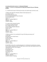
47. Retailers are always interested in determining why a customer selected their store to make a
purchase. A sporting goods retailer conducted a customer survey to determine why its customers
shopped at the store. The results are shown in the bar chart below. What proportion of the
customers responded that they shopped at the store because of the merchandise or the
convenience?

20%

Prices

50%

Merchandise

15%

Convenience

15%

Other

0%

a)
b)
c)
d)

10%

20%

30%
Responses

40%

50%

60%

35%
50%
65%
85%

ANSWER:
c
TYPE: MC DIFFICULTY: Easy
KEYWORDS: bar chart, interpretation

SCENARIO 2-7
The Stem-and-Leaf display below contains data on the number of months between the date a civil
suit is filed and when the case is actually adjudicated for 50 cases heard in superior court.
Stem
Leaves
1
234447899
2
22223455678889
3
0011135778
4
02345579
5
112466

6
158
48. Referring to Scenario 2-7, locate the first leaf, i.e., the lowest valued leaf with the lowest valued
stem. This represents a wait of ________ months.
ANSWER:
12
TYPE: FI DIFFICULTY: Easy
KEYWORDS: stem-and-leaf display, interpretation

Copyright ©2015 Pearson Education, Inc.


2-16

Organizing and Visualizing Variables

49. Referring to Scenario 2-7, the civil suit with the longest wait between when the suit was filed and
when it was adjudicated had a wait of ________ months.
ANSWER:
68
TYPE: FI DIFFICULTY: Easy
KEYWORDS: stem-and-leaf display, interpretation
50. Referring to Scenario 2-7, the civil suit with the fourth shortest waiting time between when the
suit was filed and when it was adjudicated had a wait of ________ months.
ANSWER:
14
TYPE: FI DIFFICULTY: Moderate
KEYWORDS: stem-and-leaf display, interpretation
51. Referring to Scenario 2-7, ________ percent of the cases were adjudicated within the first 2
years.

ANSWER:
30
TYPE: FI DIFFICULTY: Moderate
KEYWORDS: stem-and-leaf display, interpretation
52. Referring to Scenario 2-7, ________ percent of the cases were not adjudicated within the first 4
years.
ANSWER:
20
TYPE: FI DIFFICULTY: Moderate
KEYWORDS: stem-and-leaf display, interpretation
53. Referring to Scenario 2-7, if a frequency distribution with equal sized classes was made from this
data, and the first class was "10 but less than 20," the frequency of that class would be ________.
ANSWER:
9
TYPE: FI DIFFICULTY: Easy
KEYWORDS: stem-and-leaf display, interpretation
54.

Referring to Scenario 2-7, if a frequency distribution with equal sized classes was made from
this data, and the first class was "10 but less than 20," the relative frequency of the third class
would be ________.

ANSWER:
0.20 or 20% or 10/50
TYPE: FI DIFFICULTY: Moderate
KEYWORDS: relative frequency distribution

Copyright ©2015 Pearson Education, Inc.

Organizing and Visualizing Variables

2-17

55. Referring to Scenario 2-7, if a frequency distribution with equal sized classes was made from this
data, and the first class was "10 but less than 20," the cumulative percentage of the second class
would be ________.
ANSWER:
46% or 0.46 or 23/50
TYPE: FI DIFFICULTY: Moderate
KEYWORDS: cumulative percentage distribution

SCENARIO 2-8
The Stem-and-Leaf display represents the number of times in a year that a random sample of 100
"lifetime" members of a health club actually visited the facility.
Stem
Leaves
0
012222233333344566666667789999
1
1111222234444455669999
2
00011223455556889
3
0000446799
4
011345567
5
0077
6

8
7
67
8
3
9
0247
56. Referring to Scenario 2-8, the person who has the largest leaf associated with the smallest stem
visited the facility ________ times.
ANSWER:
9
TYPE: FI DIFFICULTY: Moderate
KEYWORDS: stem-and-leaf display, interpretation
57. Referring to Scenario 2-8, the person who visited the health club less than anyone else in the
sample visited the facility ________ times.
ANSWER:
0 or no
TYPE: FI DIFFICULTY: Easy
KEYWORDS: stem-and-leaf display, interpretation
58. Referring to Scenario 2-8, the person who visited the health club more than anyone else in the
sample visited the facility ________ times.
ANSWER:
97
TYPE: FI DIFFICULTY: Easy
KEYWORDS: stem-and-leaf display, interpretation

Copyright ©2015 Pearson Education, Inc.


2-18

Organizing and Visualizing Variables

59. Referring to Scenario 2-8, ________ of the 100 members visited the health club at least 52 times
in a year.
ANSWER:
10
TYPE: FI DIFFICULTY: Moderate
KEYWORDS: stem-and-leaf display, interpretation
60. Referring to Scenario 2-8, ________ of the 100 members visited the health club no more than 12
times in a year.
ANSWER:
38
TYPE: FI DIFFICULTY: Moderate
KEYWORDS: stem-and-leaf display, interpretation
61. Referring to Scenario 2-8, if a frequency distribution with equal sized classes was made from this
data, and the first class was "0 but less than 10," the frequency of the fifth class would be
________.
ANSWER:
9
TYPE: FI DIFFICULTY: Moderate
KEYWORDS: stem-and-leaf display, frequency distribution
62. Referring to Scenario 2-8, if a frequency distribution with equal sized classes was made from this
data, and the first class was "0 but less than 10," the relative frequency of the last class would be
________.
ANSWER:
4% or 0.04 or 4/100
TYPE: FI DIFFICULTY: Moderate
KEYWORDS: stem-and-leaf display, relative frequency distribution
63. Referring to Scenario 2-8, if a frequency distribution with equal sized classes was made from this

data, and the first class was "0 but less than 10," the cumulative percentage of the next-to-last
class would be ________.
ANSWER:
96% or 0.96 or 96/100
TYPE: FI DIFFICULTY: Moderate
KEYWORDS: stem-and-leaf display, cumulative percentage distribution

Copyright ©2015 Pearson Education, Inc.


Organizing and Visualizing Variables

2-19

64. Referring to Scenario 2-8, if a frequency distribution with equal sized classes was made from this
data, and the first class was "0 but less than 10," the class midpoint of the third class would be
________.
ANSWER:
25 or (20+30)/2
TYPE: FI DIFFICULTY: Moderate
KEYWORDS: stem-and-leaf display, class midpoint

SCENARIO 2-9
The frequency distribution below represents the rents of 250 randomly selected federally subsidized
apartments in a small town.
Rent in $
Frequency
1,100 but less than 1,200 113
1,200 but less than 1,300 85
1,300 but less than 1,400 32

1,400 but less than 1,500 16
1,500 but less than 1,600 4
65. Referring to Scenario 2-9, ________ apartments rented for at least $1,200 but less than $1,400.
ANSWER:
117
TYPE: FI DIFFICULTY: Easy
KEYWORDS: frequency distribution
66. Referring to Scenario 2-9, ________ percent of the apartments rented for $1,400 or more.
ANSWER:
8% or 20/250
TYPE: FI DIFFICULTY: Easy
KEYWORDS: frequency distribution, cumulative percentage distribution
67. Referring to Scenario 2-9, ________ percent of the apartments rented for at least $1,300.
ANSWER:
20.8% or 52/250
TYPE: FI DIFFICULTY: Moderate
KEYWORDS: frequency distribution, cumulative percentage distribution
68. Referring to Scenario 2-9, the class midpoint of the second class is ________.
ANSWER:
1,250
TYPE: FI DIFFICULTY: Easy
KEYWORDS: frequency distribution, class midpoint

Copyright ©2015 Pearson Education, Inc.


2-20

Organizing and Visualizing Variables

69. Referring to Scenario 2-9, the relative frequency of the second class is ________.
ANSWER:
85/250 or 17/50 or 34% or 0.34
TYPE: FI DIFFICULTY: Easy
KEYWORDS: frequency distribution, relative frequency distribution
70. Referring to Scenario 2-9, the percentage of apartments renting for less than $1,400 is ________.
ANSWER:
230/250 or 23/25 or 92% or 0.92
TYPE: FI DIFFICULTY: Moderate
KEYWORDS: frequency distribution, cumulative percentage distribution

SCENARIO 2-10
The histogram below represents scores achieved by 200 job applicants on a personality profile.
0.30

Rel.Freq.

0.20

0.20

0.20

0.20

0.10

0.10

0.10

0.10

0.10

0.00
0

10

20

30

40

50

60

70

71. Referring to the histogram from Scenario 2-10, ________ percent of the job applicants scored
between 10 and 20.
ANSWER:
20%
TYPE: FI DIFFICULTY: Easy
KEYWORDS: histogram, percentage distribution
72. Referring to the histogram from Scenario 2-10, ________ percent of the job applicants scored
below 50.

ANSWER:
80%
TYPE: FI DIFFICULTY: Moderate
KEYWORDS: histogram, percentage distribution
Copyright ©2015 Pearson Education, Inc.


Organizing and Visualizing Variables

2-21

73. Referring to the histogram from Scenario 2-10, the number of job applicants who scored between
30 and below 60 is _______.
ANSWER:
80
TYPE: FI DIFFICULTY: Moderate
KEYWORDS: histogram
74. Referring to the histogram from Scenario 2-10, the number of job applicants who scored 50 or
above is _______.
ANSWER:
40
TYPE: FI DIFFICULTY: Moderate
KEYWORDS: histogram
75. Referring to the histogram from Scenario 2-10, 90% of the job applicants scored above or equal
to ________.
ANSWER:
10
TYPE: FI DIFFICULTY: Moderate
KEYWORDS: histogram, cumulative percentage distribution
76. Referring to the histogram from Scenario 2-10, half of the job applicants scored below

________.
ANSWER:
30
TYPE: FI DIFFICULTY: Moderate
KEYWORDS: histogram, cumulative percentage distribution
77. Referring to the histogram from Scenario 2-10, _______ percent of the applicants scored below
20 or at least 50.
ANSWER:
50%
TYPE: FI DIFFICULTY: Moderate
KEYWORDS: histogram, cumulative percentage distribution
78. Referring to the histogram from Scenario 2-10, _______ percent of the applicants scored
between 20 and below 50.
ANSWER:
50%
TYPE: FI DIFFICULTY: Moderate
KEYWORDS: histogram, cumulative percentage distribution

Copyright ©2015 Pearson Education, Inc.


2-22

Organizing and Visualizing Variables

SCENARIO 2-11
The ordered array below resulted from selecting a sample of 25 batches of 500 computer chips and
determining how many in each batch were defective.
Defects
1 2

4
17 20 21

4
23

5
23

5
25

6
26

7
27

9
27

9
28

12
29

12
29

15

79. Referring to Scenario 2-11, if a frequency distribution for the defects data is constructed, using
"0 but less than 5" as the first class, the frequency of the “20 but less than 25” class would be
________.
ANSWER:
4
TYPE: FI DIFFICULTY: Easy
KEYWORDS: frequency distribution
80. Referring to Scenario 2-11, if a frequency distribution for the defects data is constructed, using
"0 but less than 5" as the first class, the relative frequency of the “15 but less than 20” class
would be ________.
ANSWER:
0.08 or 8% or 2/25
TYPE: FI DIFFICULTY: Moderate
KEYWORDS: relative frequency distribution
81. Referring to Scenario 2-11, construct a frequency distribution for the defects data, using "0 but
less than 5" as the first class.
ANSWER:
Defects
Frequency
0 but less than 5
4
5 but less than 10
6
10 but less than 15
2
15 but less than 20
2
20 but less than 25

4
25 but less than 30
7
TYPE: PR DIFFICULTY: Easy
KEYWORDS: frequency distribution

Copyright ©2015 Pearson Education, Inc.


Organizing and Visualizing Variables

2-23

82. Referring to Scenario 2-11, construct a relative frequency or percentage distribution for the
defects data, using "0 but less than 5" as the first class.
ANSWER:
Defects
Percentage
0 but less than 5
16
5 but less than 10
24
10 but less than 15
8
15 but less than 20
8
20 but less than 25
16
25 but less than 30
28

TYPE: PR DIFFICULTY: Moderate
KEYWORDS: relative frequency distribution, percentage distribution
83. Referring to Scenario 2-11, construct a cumulative percentage distribution for the defects data if
the corresponding frequency distribution uses "0 but less than 5" as the first class.
ANSWER:
Defects
CumPct
0
0
5
16
10
40
15
48
20
56
25
72
30
100
TYPE: PR DIFFICULTY: Moderate
KEYWORDS: cumulative percentage distribution

Copyright ©2015 Pearson Education, Inc.


2-24

Organizing and Visualizing Variables

84. Referring to Scenario 2-11, construct a histogram for the defects data, using "0 but less than 5" as
the first class.
ANSWER:
7

7

Frequency
6

6

5
4

4

4

3
2

2

2

1

0

0

10

5

15
Number of Defects

20

25

30

TYPE: PR DIFFICULTY: Easy
KEYWORDS: histogram, frequency distribution
85. Referring to Scenario 2-11, construct a cumulative percentage polygon for the defects data if the
corresponding frequency distribution uses "0 but less than 5" as the first class.

ANSWER:
Cumulative Percentage Polygon
100%
90%
80%
70%
60%
50%
40%
30%

20%
10%
0%
0

5

10

15

20

25

Number of Defects

TYPE: PR DIFFICULTY: Moderate
KEYWORDS: cumulative percentage polygon
Copyright ©2015 Pearson Education, Inc.

30


Organizing and Visualizing Variables

2-25

86. The point halfway between the boundaries of each class interval in a grouped frequency
distribution is called the _______.

ANSWER:
class midpoint
TYPE: FI DIFFICULTY: Easy
KEYWORDS: cumulative percentage polygon, frequency distribution
87. A _______ is a vertical bar chart in which the rectangular bars are constructed at the boundaries
of each class interval.
ANSWER:
histogram
TYPE: FI DIFFICULTY: Easy
KEYWORDS: histogram
88. It is essential that each class grouping or interval in a frequency distribution be ________ and
________.
ANSWER:
non-overlapping and of equal width
TYPE: FI DIFFICULTY: Moderate
KEYWORDS: frequency distribution, class interval
89. In order to compare one large set of numerical data to another, a ________ distribution must be
developed from the frequency distribution.
ANSWER:
relative frequency or percentage
TYPE: FI DIFFICULTY: Easy
KEYWORDS: relative frequency distribution, percentage distribution
90. When comparing two or more large sets of numerical data, the distributions being developed
should use the same ________.
ANSWER:
class boundaries.
TYPE: FI DIFFICULTY: Easy
KEYWORDS: class boundaries
91. The width of each class grouping or interval in a frequency distribution should be ________.
ANSWER:

the same or equal
TYPE: FI DIFFICULTY: Easy
KEYWORDS: class interval, frequency distribution

Copyright ©2015 Pearson Education, Inc.