Chapter 4 long term financial planning and growth

On February 11, 2000, JetBlue Airways took to the sky.

financed its rapid growth. The increased debt strained

The company, which started as a low-cost commuter

the company’s cash flow. During the fourth quarter

airline, offered such amenities as leather seats and free

of 2005 and the first quarter of 2006, JetBlue posted

satellite TV to all passengers. To the surprise of many

a loss when other airlines were beginning to increase

people, the company took off. During a period of tur-

net income.

moil and huge losses for most companies in the indus-

As JetBlue’s experience shows, proper manage-

try, JetBlue posted profits for 19 consecutive quarters

ment of growth is vital. This chapter emphasizes the

and became the airline darling of Wall Street investors.

importance of

Unfortunately, it is said that what goes up must come

planning for

down, and so it went for JetBlue. The company altered

the future and

DIGITAL STUDY TOOLS

its strategy when it changed its fleet to have more than

discusses some

one type of aircraft. It continued to expand aggres-

tools firms use to

sively while fuel prices were soaring. Due in part to the

think about, and

• Self-Study Software
• Multiple-Choice Quizzes
• Flashcards for Testing and Key
Terms

company’s rapid expansion, its on-time flights were

manage, growth.

Visit us at www.mhhe.com/rwj

the second worst in the industry.
Another problem caused by the rapid expansion
was JetBlue’s debt, which ballooned as the company

A lack of effective long-range planning is a commonly cited reason for financial distress
and failure. As we discuss in this chapter, long-range planning is a means of systematically
thinking about the future and anticipating possible problems before they arrive. There are no
magic mirrors, of course, so the best we can hope for is a logical and organized procedure
for exploring the unknown. As one member of GM’s board was heard to say, “Planning is a
process that at best helps the firm avoid stumbling into the future backward.”
Financial planning establishes guidelines for change and growth in a firm. It normally
focuses on the big picture. This means it is concerned with the major elements of a firm’s
financial and investment policies without examining the individual components of those
policies in detail.
Our primary goals in this chapter are to discuss financial planning and to illustrate the
interrelatedness of the various investment and financing decisions a firm makes. In the
chapters ahead, we will examine in much more detail how these decisions are made.
We first describe what is usually meant by financial planning. For the most part, we talk about
long-term planning. Short-term financial planning is discussed in a later chapter. We examine
what the firm can accomplish by developing a long-term financial plan. To do this, we develop a

Financial Statements and Long-Term Financial Planning P A R T 2

4

LONG-TERM FINANCIAL

PLANNING AND GROWTH

89

ros3062x_Ch04.indd 89

2/23/07 9:59:29 PM


90

PA RT 2

Financial Statements and Long-Term Financial Planning

simple but useful long-range planning technique: the percentage of sales approach. We describe
how to apply this approach in some simple cases, and we discuss some extensions.
To develop an explicit financial plan, managers must establish certain basic elements of
the firm’s financial policy:
1. The firm’s needed investment in new assets: This will arise from the investment
opportunities the firm chooses to undertake, and it is the result of the firm’s capital
budgeting decisions.
2. The degree of financial leverage the firm chooses to employ: This will determine the
amount of borrowing the firm will use to finance its investments in real assets. This is
the firm’s capital structure policy.
3. The amount of cash the firm thinks is necessary and appropriate to pay shareholders:
This is the firm’s dividend policy.
4. The amount of liquidity and working capital the firm needs on an ongoing basis: This
is the firm’s net working capital decision.
As we will see, the decisions a firm makes in these four areas will directly affect its future

profitability, need for external financing, and opportunities for growth.
A key lesson to be learned from this chapter is that a firm’s investment and financing policies interact and thus cannot truly be considered in isolation from one another. The types and
amounts of assets a firm plans on purchasing must be considered along with the firm’s ability
to raise the capital necessary to fund those investments. Many business students are aware of
the classic three Ps (or even four Ps) of marketing. Not to be outdone, financial planners have
no fewer than six Ps: Proper Prior Planning Prevents Poor Performance.
Financial planning forces the corporation to think about goals. A goal frequently
espoused by corporations is growth, and almost all firms use an explicit, companywide
growth rate as a major component of their long-term financial planning. For example, in
May 2006, Toyota Motor announced that it planned to sell about 10.3 million vehicles in
2010, an increase of a million cars from its 2005 sales. The company expected a 35 percent
sales increase in North America, while sales were expected to grow at 7 percent in Japan.
There are direct connections between the growth a company can achieve and its financial policy. In the following sections, we show how financial planning models can be used
to better understand how growth is achieved. We also show how such models can be used
to establish the limits on possible growth.

4.1 What Is Financial Planning?
Financial planning formulates the way in which financial goals are to be achieved. A
financial plan is thus a statement of what is to be done in the future. Most decisions have
long lead times, which means they take a long time to implement. In an uncertain world,
this requires that decisions be made far in advance of their implementation. If a firm wants
to build a factory in 2010, for example, it might have to begin lining up contractors and
financing in 2008 or even earlier.

GROWTH AS A FINANCIAL MANAGEMENT GOAL
Because the subject of growth will be discussed in various places in this chapter, we need
to start out with an important warning: Growth, by itself, is not an appropriate goal for the
financial manager. Clothing retailer J. Peterman Co., whose quirky catalogs were made
famous on the TV show Seinfeld, learned this lesson the hard way. Despite its strong brand

ros3062x_Ch04.indd 90

2/9/07 10:53:48 AM


91

C H A P T E R 4 Long-Term Financial Planning and Growth

name and years of explosive revenue growth, the company was ultimately forced to file for
bankruptcy—the victim of an overly ambitious, growth-oriented expansion plan.
Amazon.com, the big online retailer, is another example. At one time, Amazon’s motto
seemed to be “growth at any cost.” Unfortunately, what really grew rapidly for the company were losses. Amazon refocused its business, explicitly sacrificing growth in the hope
of achieving profitability. The plan seems to be working as Amazon.com turned a profit for
the first time in the third quarter of 2003.
As we discussed in Chapter 1, the appropriate goal is increasing the market value of the
owners’ equity. Of course, if a firm is successful in doing this, then growth will usually
result. Growth may thus be a desirable consequence of good decision making, but it is not
an end unto itself. We discuss growth simply because growth rates are so commonly used
in the planning process. As we will see, growth is a convenient means of summarizing
various aspects of a firm’s financial and investment policies. Also, if we think of growth as
growth in the market value of the equity in the firm, then goals of growth and increasing
the market value of the equity in the firm are not all that different.

You can find
growth rates under the
research links at
www.investor.reuters.com
and finance.yahoo.com.

DIMENSIONS OF FINANCIAL PLANNING
It is often useful for planning purposes to think of the future as having a short run and a
long run. The short run, in practice, is usually the coming 12 months. We focus our attention on financial planning over the long run, which is usually taken to be the coming two to
five years. This time period is called the planning horizon, and it is the first dimension of
the planning process that must be established.
In drawing up a financial plan, all of the individual projects and investments the firm
will undertake are combined to determine the total needed investment. In effect, the smaller
investment proposals of each operational unit are added up, and the sum is treated as one
big project. This process is called aggregation. The level of aggregation is the second
dimension of the planning process that needs to be determined.
Once the planning horizon and level of aggregation are established, a financial plan
requires inputs in the form of alternative sets of assumptions about important variables. For
example, suppose a company has two separate divisions: one for consumer products and
one for gas turbine engines. The financial planning process might require each division to
prepare three alternative business plans for the next three years:

planning horizon
The long-range time
period on which the
financial planning process focuses (usually the
next two to five years).

aggregation
The process by which
smaller investment proposals of each of a firm’s
operational units are
added up and treated as
one big project.

1. A worst case: This plan would require making relatively pessimistic assumptions

about the company’s products and the state of the economy. This kind of disaster planning would emphasize a division’s ability to withstand significant economic adversity,
and it would require details concerning cost cutting and even divestiture and liquidation. For example, sales of SUVs were sluggish in 2006 because of high gas prices.
That left auto manufacturers like Ford and GM with large inventories and resulted in
large price cuts and discounts.
2. A normal case: This plan would require making the most likely assumptions about the
company and the economy.
3. A best case: Each division would be required to work out a case based on optimistic
assumptions. It could involve new products and expansion and would then detail the
financing needed to fund the expansion.
In this example, business activities are aggregated along divisional lines, and the planning horizon is three years. This type of planning, which considers all possible events,
is particularly important for cyclical businesses (businesses with sales that are strongly
affected by the overall state of the economy or business cycles).

ros3062x_Ch04.indd 91

2/9/07 10:53:48 AM


92

PA RT 2

Financial Statements and Long-Term Financial Planning

WHAT CAN PLANNING ACCOMPLISH?
Because a company is likely to spend a lot of time examining the different scenarios that
will become the basis for its financial plan, it seems reasonable to ask what the planning
process will accomplish.

Examining Interactions As we discuss in greater detail in the following pages, the

financial plan must make explicit the linkages between investment proposals for the different operating activities of the firm and its available financing choices. In other words, if the
firm is planning on expanding and undertaking new investments and projects, where will
the financing be obtained to pay for this activity?
Exploring Options The financial plan allows the firm to develop, analyze, and compare
many different scenarios in a consistent way. Various investment and financing options
can be explored, and their impact on the firm’s shareholders can be evaluated. Questions
concerning the firm’s future lines of business and optimal financing arrangements are
addressed. Options such as marketing new products or closing plants might be evaluated.
Avoiding Surprises Financial planning should identify what may happen to the firm if
different events take place. In particular, it should address what actions the firm will take if
things go seriously wrong or, more generally, if assumptions made today about the future
are seriously in error. As physicist Niels Bohr once observed, “Prediction is very difficult,
particularly when it concerns the future.” Thus, one purpose of financial planning is to
avoid surprises and develop contingency plans.
For example, in December 2005, Microsoft lowered the sales numbers on its new Xbox
360 from 3 million units to 2.5–2.75 million units during the first 90 days it was on the
market. The fall in sales did not occur because of a lack of demand. Instead, Microsoft
experienced a shortage of parts. Thus, a lack of planning for sales growth can be a problem
for even the biggest companies.
Ensuring Feasibility and Internal Consistency Beyond a general goal of creating
value, a firm will normally have many specific goals. Such goals might be couched in
terms of market share, return on equity, financial leverage, and so on. At times, the linkages between different goals and different aspects of a firm’s business are difficult to see.
Not only does a financial plan make explicit these linkages, but it also imposes a unified
structure for reconciling goals and objectives. In other words, financial planning is a way
of verifying that the goals and plans made for specific areas of a firm’s operations are feasible and internally consistent. Conflicting goals will often exist. To generate a coherent
plan, goals and objectives will therefore have to be modified, and priorities will have to be
established.
For example, one goal a firm might have is 12 percent growth in unit sales per year.
Another goal might be to reduce the firm’s total debt ratio from 40 to 20 percent. Are these
two goals compatible? Can they be accomplished simultaneously? Maybe yes, maybe no.

As we will discuss, financial planning is a way of finding out just what is possible—and,
by implication, what is not possible.
Conclusion Probably the most important result of the planning process is that it forces
managers to think about goals and establish priorities. In fact, conventional business wisdom holds that financial plans don’t work, but financial planning does. The future is inherently unknown. What we can do is establish the direction in which we want to travel and

ros3062x_Ch04.indd 92

2/9/07 10:53:49 AM


93

C H A P T E R 4 Long-Term Financial Planning and Growth

make some educated guesses about what we will find along the way. If we do a good job,
we won’t be caught off guard when the future rolls around.

Concept Questions
4.1a What are the two dimensions of the financial planning process?
4.1b Why should firms draw up financial plans?

Financial Planning Models:
A First Look

4.2

Just as companies differ in size and products, the financial planning process will differ
from firm to firm. In this section, we discuss some common elements in financial plans and
develop a basic model to illustrate these elements. What follows is just a quick overview;
later sections will take up the various topics in more detail.

A FINANCIAL PLANNING MODEL: THE INGREDIENTS
Most financial planning models require the user to specify some assumptions about the
future. Based on those assumptions, the model generates predicted values for many other
variables. Models can vary quite a bit in complexity, but almost all have the elements we
discuss next.

Sales Forecast Almost all financial plans require an externally supplied sales forecast.
In our models that follow, for example, the sales forecast will be the “driver,” meaning that
the user of the planning model will supply this value, and most other values will be calculated based on it. This arrangement is common for many types of business; planning will
focus on projected future sales and the assets and financing needed to support those sales.
Frequently, the sales forecast will be given as the growth rate in sales rather than as an
explicit sales figure. These two approaches are essentially the same because we can calculate
projected sales once we know the growth rate. Perfect sales forecasts are not possible, of course,
because sales depend on the uncertain future state of the economy. To help a firm come up with
its projections, some businesses specialize in macroeconomic and industry projections.
As we discussed previously, we frequently will be interested in evaluating alternative
scenarios, so it isn’t necessarily crucial that the sales forecast be accurate. In such cases,
our goal is to examine the interplay between investment and financing needs at different
possible sales levels, not to pinpoint what we expect to happen.
Pro Forma Statements A financial plan will have a forecast balance sheet, income
statement, and statement of cash flows. These are called pro forma statements, or pro
formas for short. The phrase pro forma literally means “as a matter of form.” In our case,
this means the financial statements are the form we use to summarize the different events
projected for the future. At a minimum, a financial planning model will generate these
statements based on projections of key items such as sales.
In the planning models we will describe, the pro formas are the output from the financial planning model. The user will supply a sales figure, and the model will generate the
resulting income statement and balance sheet.

ros3062x_Ch04.indd 93

Spreadsheets to
use for pro forma statements
can be obtained at
www.jaxworks.com.

2/9/07 10:53:49 AM


94

PA RT 2

Financial Statements and Long-Term Financial Planning

Asset Requirements The plan will describe projected capital spending. At a minimum, the
projected balance sheet will contain changes in total fixed assets and net working capital. These
changes are effectively the firm’s total capital budget. Proposed capital spending in different
areas must thus be reconciled with the overall increases contained in the long-range plan.
Financial Requirements The plan will include a section about the necessary financing
arrangements. This part of the plan should discuss dividend policy and debt policy. Sometimes firms will expect to raise cash by selling new shares of stock or by borrowing. In
this case, the plan will have to consider what kinds of securities have to be sold and what
methods of issuance are most appropriate. These are subjects we consider in Part 6 of our
book, where we discuss long-term financing, capital structure, and dividend policy.
The Plug After the firm has a sales forecast and an estimate of the required spending on
assets, some amount of new financing will often be necessary because projected total assets
will exceed projected total liabilities and equity. In other words, the balance sheet will no
longer balance.
Because new financing may be necessary to cover all of the projected capital spending,
a financial “plug” variable must be selected. The plug is the designated source or sources

of external financing needed to deal with any shortfall (or surplus) in financing and thereby
bring the balance sheet into balance.
For example, a firm with a great number of investment opportunities and limited cash
flow may have to raise new equity. Other firms with few growth opportunities and ample
cash flow will have a surplus and thus might pay an extra dividend. In the first case, external equity is the plug variable. In the second, the dividend is used.
Economic Assumptions The plan will have to state explicitly the economic environment in which the firm expects to reside over the life of the plan. Among the more important economic assumptions that will have to be made are the level of interest rates and the
firm’s tax rate.

A SIMPLE FINANCIAL PLANNING MODEL
We can begin our discussion of long-term planning models with a relatively simple example. The Computerfield Corporation’s financial statements from the most recent year are
as follows:
COMPUTERFIELD CORPORATION
Financial Statements

Income Statement
Sales
Costs
Net income

$1,000
800
$ 200

Balance Sheet
Assets

$500

Total

$500

Debt
Equity
Total

$250
250
$500

Unless otherwise stated, the financial planners at Computerfield assume that all variables are tied directly to sales and current relationships are optimal. This means that all
items will grow at exactly the same rate as sales. This is obviously oversimplified; we use
this assumption only to make a point.
Suppose sales increase by 20 percent, rising from $1,000 to $1,200. Planners would
then also forecast a 20 percent increase in costs, from $800 to $800 ϫ 1.2 ϭ $960. The pro
forma income statement would thus be:

ros3062x_Ch04.indd 94

2/9/07 10:53:50 AM


C H A P T E R 4 Long-Term Financial Planning and Growth

95

Pro Forma
Income Statement

Sales

Costs
Net income

$1,200
960
$ 240

The assumption that all variables will grow by 20 percent lets us easily construct the pro
forma balance sheet as well:
Pro Forma Balance Sheet

Assets

$600 (ϩ100)

Total

$600 (ϩ100)

Debt
Equity
Total

$300 (ϩ 50)
300 (ϩ 50)
$600 (ϩ100)

Notice that we have simply increased every item by 20 percent. The numbers in parentheses are the dollar changes for the different items.
Now we have to reconcile these two pro formas. How, for example, can net income be
equal to $240 and equity increase by only $50? The answer is that Computerfield must

have paid out the difference of $240 Ϫ 50 ϭ $190, possibly as a cash dividend. In this case,
dividends are the plug variable.
Suppose Computerfield does not pay out the $190. In this case, the addition to retained
earnings is the full $240. Computerfield’s equity will thus grow to $250 (the starting
amount) plus $240 (net income), or $490, and debt must be retired to keep total assets
equal to $600.
With $600 in total assets and $490 in equity, debt will have to be $600 Ϫ 490 ϭ $110.
Because we started with $250 in debt, Computerfield will have to retire $250 Ϫ 110 ϭ
$140 in debt. The resulting pro forma balance sheet would look like this:

Planware
provides insight into cash
flow forecasting in its “White
Papers” section
(www.planware.org).

Pro Forma Balance Sheet

Assets

$600 (ϩ100)

Total

$600 (ϩ100)

Debt
Equity
Total

$110 (Ϫ140)
490 (ϩ240)
$600 (ϩ100)

In this case, debt is the plug variable used to balance projected total assets and liabilities.
This example shows the interaction between sales growth and financial policy. As sales
increase, so do total assets. This occurs because the firm must invest in net working capital
and fixed assets to support higher sales levels. Because assets are growing, total liabilities
and equity (the right side of the balance sheet) will grow as well.
The thing to notice from our simple example is that the way the liabilities and owners’
equity change depends on the firm’s financing policy and its dividend policy. The growth
in assets requires that the firm decide on how to finance that growth. This is strictly a
managerial decision. Note that in our example, the firm needed no outside funds. This
won’t usually be the case, so we explore a more detailed situation in the next section.

Concept Questions
4.2a What are the basic components of a financial plan?
4.2b Why is it necessary to designate a plug in a financial planning model?

ros3062x_Ch04.indd 95

2/9/07 10:53:51 AM


96

PA RT 2

Financial Statements and Long-Term Financial Planning

4.3 The Percentage of Sales Approach

percentage of sales
approach
A financial planning method
in which accounts are varied depending on a firm’s
predicted sales level.

dividend payout ratio
The amount of cash
paid out to shareholders
divided by net income.

In the previous section, we described a simple planning model in which every item increased
at the same rate as sales. This may be a reasonable assumption for some elements. For others,
such as long-term borrowing, it probably is not: The amount of long-term borrowing is something set by management, and it does not necessarily relate directly to the level of sales.
In this section, we describe an extended version of our simple model. The basic idea is
to separate the income statement and balance sheet accounts into two groups—those that
vary directly with sales and those that do not. Given a sales forecast, we will then be able
to calculate how much financing the firm will need to support the predicted sales level.
The financial planning model we describe next is based on the percentage of sales
approach. Our goal here is to develop a quick and practical way of generating pro forma
statements. We defer discussion of some “bells and whistles” to a later section.

THE INCOME STATEMENT
We start out with the most recent income statement for the Rosengarten Corporation, as
that shown in Table 4.1. Notice we have still simplified things by including costs, depreciation, and interest in a single cost figure.
Rosengarten has projected a 25 percent increase in sales for the coming year, so we are
anticipating sales of $1,000 ϫ 1.25 ϭ $1,250. To generate a pro forma income statement,
we assume that total costs will continue to run at $800ր1,000 ϭ 80% of sales. With this

assumption, Rosengarten’s pro forma income statement is shown in Table 4.2. The effect
here of assuming that costs are a constant percentage of sales is to assume that the profit
margin is constant. To check this, notice that the profit margin was $132ր1,000 ϭ 13.2%.
In our pro forma, the profit margin is $165ր1,250 ϭ 13.2%; so it is unchanged.
Next, we need to project the dividend payment. This amount is up to Rosengarten’s
management. We will assume Rosengarten has a policy of paying out a constant fraction of
net income in the form of a cash dividend. For the most recent year, the dividend payout

TABLE 4.1

ROSENGARTEN CORPORATION
Income Statement

Sales

$1,000

Costs

800

Taxable income

$ 200

Taxes (34%)
Net income
Dividends

68

$ 132
$44

Addition to retained earnings

TABLE 4.2

ros3062x_Ch04.indd 96

88

ROSENGARTEN CORPORATION
Pro Forma Income Statement

Sales (projected)
Costs (80% of sales)
Taxable income
Taxes (34%)

$1,250
1,000
$ 250
85

Net income

$ 165

2/9/07 10:53:52 AM

97

C H A P T E R 4 Long-Term Financial Planning and Growth

ratio was this:
Dividend payout ratio ϭ Cash dividends/Net income
ϭ $44ր132 ϭ 33 1/3%

[4.1]

We can also calculate the ratio of the addition to retained earnings to net income:
Addition to retained earnings/Net income ϭ $88ր132 ϭ 66 2ր3%
This ratio is called the retention ratio or plowback ratio, and it is equal to 1 minus the
dividend payout ratio because everything not paid out is retained. Assuming that the
payout ratio is constant, here are the projected dividends and addition to retained earnings:
Projected dividends paid to shareholders ϭ $165 ϫ 1ր3 ϭ $ 55
Projected addition to retained earnings ϭ $165 ϫ 2ր3 ϭ 110
$165

retention ratio
The addition to retained
earnings divided by net
income. Also called the
plowback ratio.

THE BALANCE SHEET
To generate a pro forma balance sheet, we start with the most recent statement, as shown
in Table 4.3.
On our balance sheet, we assume that some items vary directly with sales and others do

not. For items that vary with sales, we express each as a percentage of sales for the year
just completed. When an item does not vary directly with sales, we write “n/a” for “not
applicable.”
For example, on the asset side, inventory is equal to 60 percent of sales ($600/1,000)
for the year just ended. We assume this percentage applies to the coming year, so for each
$1 increase in sales, inventory will rise by $.60. More generally, the ratio of total assets to
sales for the year just ended is $3,000/1,000 ϭ 3, or 300%.
This ratio of total assets to sales is sometimes called the capital intensity ratio. It tells
us the amount of assets needed to generate $1 in sales; so the higher the ratio is, the more
capital-intensive is the firm. Notice also that this ratio is just the reciprocal of the total asset
turnover ratio we defined in the last chapter.

capital intensity ratio
A firm’s total assets
divided by its sales, or the
amount of assets needed
to generate $1 in sales.

TABLE 4.3
ROSENGARTEN CORPORATION
Balance Sheet

Assets

Current assets
Cash
Accounts receivable
Inventory
Total
Fixed assets

Net plant and equipment

Total assets

ros3062x_Ch04.indd 97

Liabilities and Owners’ Equity
$

Percentage
of Sales

$ 160
440
600
$1,200

16%
44
60
120

$1,800

180

$3,000

300%

Current liabilities
Accounts payable
Notes payable
Total
Long-term debt
Owners’ equity
Common stock and paid-in
surplus
Retained earnings
Total
Total liabilities and owners’ equity

$

Percentage
of Sales

$ 300
100
$ 400
$ 800

30%
n/a
n/a
n/a

$ 800
1,000
$1,800

$3,000

n/a
n/a
n/a
n/a

2/9/07 10:53:53 AM


98

PA RT 2

Financial Statements and Long-Term Financial Planning

For Rosengarten, assuming that this ratio is constant, it takes $3 in total assets to generate $1 in sales (apparently Rosengarten is in a relatively capital-intensive business). Therefore, if sales are to increase by $100, Rosengarten will have to increase total assets by three
times this amount, or $300.
On the liability side of the balance sheet, we show accounts payable varying with sales.
The reason is that we expect to place more orders with our suppliers as sales volume
increases, so payables will change “spontaneously” with sales. Notes payable, on the other
hand, represent short-term debt such as bank borrowing. This item will not vary unless we
take specific actions to change the amount, so we mark it as “n/a.”
Similarly, we use “n/a” for long-term debt because it won’t automatically change with
sales. The same is true for common stock and paid-in surplus. The last item on the right
side, retained earnings, will vary with sales, but it won’t be a simple percentage of sales.
Instead, we will explicitly calculate the change in retained earnings based on our projected
net income and dividends.
We can now construct a partial pro forma balance sheet for Rosengarten. We do this
by using the percentages we have just calculated wherever possible to calculate the projected amounts. For example, net fixed assets are 180 percent of sales; so, with a new

sales level of $1,250, the net fixed asset amount will be 1.80 ϫ $1,250 ϭ $2,250, representing an increase of $2,250 Ϫ 1,800 ϭ $450 in plant and equipment. It is important to
note that for items that don’t vary directly with sales, we initially assume no change and
simply write in the original amounts. The result is shown in Table 4.4. Notice that the
change in retained earnings is equal to the $110 addition to retained earnings we calculated earlier.
Inspecting our pro forma balance sheet, we notice that assets are projected to increase
by $750. However, without additional financing, liabilities and equity will increase by only
$185, leaving a shortfall of $750 Ϫ 185 ϭ $565. We label this amount external financing
needed (EFN).
TABLE 4.4
ROSENGARTEN CORPORATION
Partial Pro Forma Balance Sheet

Assets

Liabilities and Owners’ Equity

Present
Year

Change from
Previous Year

Current assets
Cash
Accounts receivable
Inventory
Total

Present
Year

Change from
Previous Year

$ 375
100

$ 75
0

$ 475

$ 75

$ 800

$

0

$ 800

$

0

Current liabilities
$ 200
550

$ 40
110

Accounts payable
Notes payable

750

150

$1,500

$300

Long-term debt

Total

$2,250

$450

Owners’ equity

Fixed assets
Net plant and equipment

Common stock and
paid-in surplus
Retained earnings

1,110

110

$1,910

$110

Total liabilities
and owners’ equity

$3,185

$185

External financing needed

$ 565

$565

Total
Total assets

ros3062x_Ch04.indd 98

$3,750

$750

2/9/07 10:53:54 AM


99

C H A P T E R 4 Long-Term Financial Planning and Growth

A PARTICULAR SCENARIO
Our financial planning model now reminds us of one of those good news–bad news jokes.
The good news is we’re projecting a 25 percent increase in sales. The bad news is that this
isn’t going to happen unless Rosengarten can somehow raise $565 in new financing.
This is a good example of how the planning process can point out problems and potential
conflicts. If, for example, Rosengarten has a goal of not borrowing any additional funds and
not selling any new equity, then a 25 percent increase in sales is probably not feasible.
If we take the need for $565 in new financing as given, we know that Rosengarten has
three possible sources: short-term borrowing, long-term borrowing, and new equity. The
choice of some combination among these three is up to management; we will illustrate only
one of the many possibilities.
Suppose Rosengarten decides to borrow the needed funds. In this case, the firm
might choose to borrow some over the short term and some over the long term. For
example, current assets increased by $300 whereas current liabilities rose by only $75.
Rosengarten could borrow $300 Ϫ 75 ϭ $225 in short-term notes payable and leave total
net working capital unchanged. With $565 needed, the remaining $565 Ϫ 225 ϭ $340
would have to come from long-term debt. Table 4.5 shows the completed pro forma balance sheet for Rosengarten.
We have used a combination of short- and long-term debt as the plug here, but we
emphasize that this is just one possible strategy; it is not necessarily the best one by any
means. There are many other scenarios we could (and should) investigate. The various
ratios we discussed in Chapter 3 come in handy here. For example, with the scenario we
have just examined, we would surely want to examine the current ratio and the total debt

ratio to see if we were comfortable with the new projected debt levels.
Now that we have finished our balance sheet, we have all of the projected sources and
uses of cash. We could finish off our pro formas by drawing up the projected statement
of cash flows along the lines discussed in Chapter 3. We will leave this as an exercise and
instead investigate an important alternative scenario.
TABLE 4.5
ROSENGARTEN CORPORATION
Pro Forma Balance Sheet

Assets

Liabilities and Owners’ Equity

Present
Year

Change from
Previous Year

Current assets
Cash
Accounts receivable
Inventory
Total

Present
Year

Change from
Previous Year

Current liabilities
$ 200
550

$ 40
110

Accounts payable
Notes payable

750

150

$1,500

$300

Long-term debt

Total

$2,250

$450

Owners’ equity

$ 375

325

$ 75
225

$ 700

$300

$1,140

$340

$ 800

$

Fixed assets
Net plant and equipment

Common stock and
paid-in surplus
Retained earnings
Total
Total assets

ros3062x_Ch04.indd 99

$3,750

$750

Total liabilities
and owners’ equity

0

1,110

110

$1,910

$110

$3,750

$750

2/9/07 10:53:56 AM


100

PA RT 2

Financial Statements and Long-Term Financial Planning

AN ALTERNATIVE SCENARIO
The assumption that assets are a fixed percentage of sales is convenient, but it may not be

suitable in many cases. In particular, note that we effectively assumed that Rosengarten
was using its fixed assets at 100 percent of capacity because any increase in sales led to an
increase in fixed assets. For most businesses, there would be some slack or excess capacity, and production could be increased by perhaps running an extra shift. According to the
Federal Reserve, the overall capacity utilization for U.S. industrial companies in April
2006 was 81.4 percent, up from a low of 73.9 percent in 2001.
For example, in early 2006, Kia Motors announced that it would build its first manufacturing plant in North America in Georgia. This followed recent announcements by Ford
and General Motors that those companies would be closing plants in Georgia. Evidently,
both Ford and General Motors had excess capacity, whereas Kia did not.
In another example, in early 2004, Simmons announced it was closing its mattress factory in Ohio. The company stated it would increase mattress production at other plants to
compensate for the closing. Apparently, Simmons had significant excess capacity in its
production facilities.
If we assume that Rosengarten is operating at only 70 percent of capacity, then the need
for external funds will be quite different. When we say “70 percent of capacity,” we mean
that the current sales level is 70 percent of the full-capacity sales level:
Current sales ϭ $1,000 ϭ .70 ϫ Full-capacity sales
Full-capacity sales ϭ $1,000ր.70 ϭ $1,429
This tells us that sales could increase by almost 43 percent—from $1,000 to $1,429—
before any new fixed assets would be needed.
In our previous scenario, we assumed it would be necessary to add $450 in net fixed assets.
In the current scenario, no spending on net fixed assets is needed because sales are projected
to rise only to $1,250, which is substantially less than the $1,429 full-capacity level.
As a result, our original estimate of $565 in external funds needed is too high. We
estimated that $450 in net new fixed assets would be needed. Instead, no spending on new
net fixed assets is necessary. Thus, if we are currently operating at 70 percent capacity, we
need only $565 Ϫ 450 ϭ $115 in external funds. The excess capacity thus makes a considerable difference in our projections.

EXAMPLE 4.1

EFN and Capacity Usage
Suppose Rosengarten is operating at 90 percent capacity. What would sales be at full

capacity? What is the capital intensity ratio at full capacity? What is EFN in this case?
Full-capacity sales would be $1,000ր.90 ϭ $1,111. From Table 4.3, we know that fixed
assets are $1,800. At full capacity, the ratio of fixed assets to sales is this:
Fixed assets/Full-capacity sales ϭ $1,800/1,111 ϭ 1.62
So, Rosengarten needs $1.62 in fixed assets for every $1 in sales once it reaches full
capacity. At the projected sales level of $1,250, then, it needs $1,250 ϫ 1.62 ϭ $2,025 in
fixed assets. Compared to the $2,250 we originally projected, this is $225 less, so EFN is
$565 Ϫ 225 ϭ $340.
Current assets would still be $1,500, so total assets would be $1,500 ϩ 2,025 ϭ $3,525.
The capital intensity ratio would thus be $3,525/1,250 ϭ 2.82, which is less than our original value of 3 because of the excess capacity.

ros3062x_Ch04.indd 100

2/9/07 10:53:57 AM


101

C H A P T E R 4 Long-Term Financial Planning and Growth

These alternative scenarios illustrate that it is inappropriate to blindly manipulate financial statement information in the planning process. The results depend critically on the
assumptions made about the relationships between sales and asset needs. We return to this
point a little later.
One thing should be clear by now. Projected growth rates play an important role in
the planning process. They are also important to outside analysts and potential investors.
Our nearby Work the Web box shows you how to obtain growth rate estimates for real
companies.

Concept Questions
4.3a What is the basic idea behind the percentage of sales approach?

4.3b Unless it is modified, what does the percentage of sales approach assume about
fixed asset capacity usage?

External Financing and Growth

4.4

External financing needed and growth are obviously related. All other things staying the
same, the higher the rate of growth in sales or assets, the greater will be the need for external financing. In the previous section, we took a growth rate as given, and then we determined the amount of external financing needed to support that growth. In this section, we
turn things around a bit. We will take the firm’s financial policy as given and then examine
the relationship between that financial policy and the firm’s ability to finance new investments and thereby grow.
Once again, we emphasize that we are focusing on growth not because growth is
an appropriate goal; instead, for our purposes, growth is simply a convenient means of
examining the interactions between investment and financing decisions. In effect, we
assume that the use of growth as a basis for planning is just a reflection of the very high
level of aggregation used in the planning process.

EFN AND GROWTH
The first thing we need to do is establish the relationship between EFN and growth.
To do this, we introduce the simplified income statement and balance sheet for the
Hoffman Company in Table 4.6. Notice that we have simplified the balance sheet by
combining short-term and long-term debt into a single total debt figure. Effectively, we
are assuming that none of the current liabilities varies spontaneously with sales. This
assumption isn’t as restrictive as it sounds. If any current liabilities (such as accounts
payable) vary with sales, we can assume that any such accounts have been netted out
in current assets. Also, we continue to combine depreciation, interest, and costs on the
income statement.
Suppose the Hoffman Company is forecasting next year’s sales level at $600, a
$100 increase. Notice that the percentage increase in sales is $100ր500 ϭ 20%. Using
the percentage of sales approach and the figures in Table 4.6, we can prepare a pro

forma income statement and balance sheet as in Table 4.7. As Table 4.7 illustrates, at a
20 percent growth rate, Hoffman needs $100 in new assets (assuming full capacity). The
projected addition to retained earnings is $52.8, so the external financing needed (EFN)
is $100 Ϫ 52.8 ϭ $47.2.

ros3062x_Ch04.indd 101

2/9/07 10:53:58 AM


102

PA RT 2

Financial Statements and Long-Term Financial Planning

TABLE 4.6
HOFFMAN COMPANY
Income Statement and Balance Sheet

Income Statement
Sales
Costs

$500
400

Taxable income

$100

Taxes (34%)

34

Net income

$ 66

Dividends

$22

Addition to retained earnings

44
Balance Sheet

Assets

Current assets

Liabilities and Owners’ Equity

$

Percentage
of Sales

$200

40%

Total debt

Net fixed assets

300

60

Owners’ equity

Total assets

$500

100%

Total liabilities and owners’ equity

$

Percentage
of Sales

$250

n/a

250

n/a

$500

n/a

TABLE 4.7
HOFFMAN COMPANY
Pro Forma Income Statement and Balance Sheet

Income Statement
Sales (projected)

$600.0
480.0

Costs (80% of sales)
Taxable income

$120.0

Taxes (34%)

40.8

Net income

$ 79.2

Dividends

$26.4

Addition to retained earnings

52.8
Balance Sheet

Assets
$
Current assets
Net fixed assets
Total assets

Liabilities and Owners’ Equity
Percentage
of Sales

$240.0

$

40%

Total debt

360.0

60

Owners’ equity

$600.0

100%

Total liabilities and owners’ equity
External financing needed

Percentage
of Sales

$250.0

n/a

302.8

n/a

$552.8

n/a

$ 47.2

n/a

Notice that the debt–equity ratio for Hoffman was originally (from Table 4.6) equal to
$250ր250 ϭ 1.0. We will assume that the Hoffman Company does not wish to sell new
equity. In this case, the $47.2 in EFN will have to be borrowed. What will the new debt–
equity ratio be? From Table 4.7, we know that total owners’ equity is projected at $302.8.
The new total debt will be the original $250 plus $47.2 in new borrowing, or $297.2 total.
The debt–equity ratio thus falls slightly from 1.0 to $297.2ր302.8 ϭ .98.

ros3062x_Ch04.indd 102

2/9/07 10:53:59 AM


103

C H A P T E R 4 Long-Term Financial Planning and Growth

WORK THE WEB

WORK THE WEB

Calculating company growth rates can involve detailed research, and a major part of a stock analyst’s job is to
estimate them. One place to find earnings and sales growth rates on the Web is Yahoo! Finance at finance.yahoo.
com. We pulled up a quote for Minnesota Mining & Manufacturing (MMM, or 3M as it is known) and followed the
“Analyst Estimates” link. Here is an abbreviated look at the results:

As shown, analysts expect, on average, revenue (sales) of $22.77 billion in 2006, growing to $24.27 billion
in 2007, an increase of 6.6 percent. We also have the following table comparing MMM to some benchmarks:

As you can see, the estimated earnings growth rate for MMM is lower than the industry and S&P 500 over the
next five years. What does this mean for MMM stock? We’ll get to that in a later chapter.

Table 4.8 shows EFN for several different growth rates. The projected addition to
retained earnings and the projected debt–equity ratio for each scenario are also given (you
should probably calculate a few of these for practice). In determining the debt–equity
ratios, we assumed that any needed funds were borrowed, and we also assumed any surplus
funds were used to pay off debt. Thus, for the zero growth case, the debt falls by $44, from
$250 to $206. In Table 4.8, notice that the increase in assets required is simply equal to

ros3062x_Ch04.indd 103

2/9/07 10:54:13 AM


104

TABLE 4.8
Growth and Projected
EFN for the Hoffman
Company

PA RT 2

Financial Statements and Long-Term Financial Planning

Projected
Sales
Growth

Increase
in Assets

Required

Addition to
Retained
Earnings

External
Financing
Needed, EFN

Projected
Debt–Equity
Ratio

0

$44.0

Ϫ$44.0

.70

5

25

46.2

Ϫ 21.2

.77

10

50

48.4

1.6

.84

15

75

50.6

24.4

.91

20

100

52.8

47.2

.98

25

125

55.0

70.0

1.05

0%

$

Growth and Related
Financing Needed for the
Hoffman Company

Asset needs and retained earnings ($)

FIGURE 4.1
Increase
in assets
required

125

100

EFN Ͼ 0
(deficit)

75

50
44 EFN Ͻ 0
(surplus)
25

5

Projected
addition
to retained
earnings

10
15
20
Projected growth in sales (%)

25

the original assets of $500 multiplied by the growth rate. Similarly, the addition to retained
earnings is equal to the original $44 plus $44 times the growth rate.
Table 4.8 shows that for relatively low growth rates, Hoffman will run a surplus, and
its debt–equity ratio will decline. Once the growth rate increases to about 10 percent, however, the surplus becomes a deficit. Furthermore, as the growth rate exceeds approximately
20 percent, the debt–equity ratio passes its original value of 1.0.
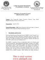
Figure 4.1 illustrates the connection between growth in sales and external financing

needed in more detail by plotting asset needs and additions to retained earnings from
Table 4.8 against the growth rates. As shown, the need for new assets grows at a much
faster rate than the addition to retained earnings, so the internal financing provided by the
addition to retained earnings rapidly disappears.
As this discussion shows, whether a firm runs a cash surplus or deficit depends on growth.
Microsoft is a good example. Its revenue growth in the 1990s was amazing, averaging well
over 30 percent per year for the decade. Growth slowed down noticeably over the 2000–
2006 period; but nonetheless, Microsoft’s combination of growth and substantial profit margins led to enormous cash surpluses. In part because Microsoft paid few or no dividends, the
cash really piled up; in 2006, Microsoft’s cash horde exceeded $38 billion.

ros3062x_Ch04.indd 104

2/9/07 10:54:17 AM


105

C H A P T E R 4 Long-Term Financial Planning and Growth

FINANCIAL POLICY AND GROWTH
Based on our preceding discussion, we see that there is a direct link between growth and
external financing. In this section, we discuss two growth rates that are particularly useful
in long-range planning.

The Internal Growth Rate The first growth rate of interest is the maximum growth rate
that can be achieved with no external financing of any kind. We will call this the internal
growth rate because this is the rate the firm can maintain with internal financing only. In
Figure 4.1, this internal growth rate is represented by the point where the two lines cross.
At this point, the required increase in assets is exactly equal to the addition to retained
earnings, and EFN is therefore zero. We have seen that this happens when the growth rate

is slightly less than 10 percent. With a little algebra (see Problem 32 at the end of the chapter), we can define this growth rate more precisely:
ROA ϫ b
Internal growth rate ϭ ____________
1 Ϫ ROA ϫ b

internal growth rate
The maximum growth rate
a firm can achieve without
external financing of any
kind.

[4.2]

Here, ROA is the return on assets we discussed in Chapter 3, and b is the plowback, or
retention, ratio defined earlier in this chapter.
For the Hoffman Company, net income was $66 and total assets were $500. ROA is thus
$66ր500 ϭ 13.2%. Of the $66 net income, $44 was retained, so the plowback ratio, b, is
$44ր66 ϭ 2ր3. With these numbers, we can calculate the internal growth rate:
ROA ϫ b
Internal growth rate ϭ ____________
1 Ϫ ROA ϫ b
.132 ϫ (2/3)
ϭ ______________
1 Ϫ .132 ϫ (2/3)
ϭ 9.65%
Thus, the Hoffman Company can expand at a maximum rate of 9.65 percent per year without external financing.

The Sustainable Growth Rate We have seen that if the Hoffman Company wishes
to grow more rapidly than at a rate of 9.65 percent per year, external financing must be
arranged. The second growth rate of interest is the maximum growth rate a firm can achieve

with no external equity financing while it maintains a constant debt–equity ratio. This rate
is commonly called the sustainable growth rate because it is the maximum rate of growth
a firm can maintain without increasing its financial leverage.
There are various reasons why a firm might wish to avoid equity sales. For example,
as we discuss in Chapter 16, new equity sales can be expensive. Alternatively, the current
owners may not wish to bring in new owners or contribute additional equity. Why a firm
might view a particular debt–equity ratio as optimal is discussed in Chapters 15 and 17; for
now, we will take it as given.
Based on Table 4.8, the sustainable growth rate for Hoffman is approximately 20 percent because the debt–equity ratio is near 1.0 at that growth rate. The precise value can be
calculated (see Problem 32 at the end of the chapter):
ROE ϫ b
Sustainable growth rate ϭ ____________
1 Ϫ ROE ϫ b

sustainable growth rate
The maximum growth rate
a firm can achieve without
external equity financing
while maintaining a constant debt–equity ratio.

[4.3]

This is identical to the internal growth rate except that ROE, return on equity, is used
instead of ROA.

ros3062x_Ch04.indd 105

2/9/07 10:54:18 AM

106

PA RT 2

Financial Statements and Long-Term Financial Planning

For the Hoffman Company, net income was $66 and total equity was $250; ROE is thus
$66/250 ϭ 26.4 percent. The plowback ratio, b, is still 2/3, so we can calculate the sustainable growth rate as follows:
ROE ϫ b
Sustainable growth rate ϭ ____________
1 Ϫ ROE ϫ b
.264 ϫ (2/3)
ϭ ______________
1 Ϫ .264 ϫ (2/3)
ϭ 21.36%
Thus, the Hoffman Company can expand at a maximum rate of 21.36 percent per year
without external equity financing.

EXAMPLE 4.2

Sustainable Growth
Suppose Hoffman grows at exactly the sustainable growth rate of 21.36 percent. What will
the pro forma statements look like?
At a 21.36 percent growth rate, sales will rise from $500 to $606.8. The pro forma
income statement will look like this:

HOFFMAN COMPANY
Pro Forma Income Statement

Sales (projected)

Costs (80% of sales)
Taxable income
Taxes (34%)
Net income
Dividends
Addition to retained earnings

$606.8
485.4
$121.4
41.3
$ 80.1
$26.7
53.4

We construct the balance sheet just as we did before. Notice, in this case, that owners’
equity will rise from $250 to $303.4 because the addition to retained earnings is $53.4.

HOFFMAN COMPANY
Pro Forma Balance Sheet

Assets
Percentage
of Sales

$
Current assets

Liabilities and Owners’ Equity

40%

Total debt

Net fixed assets

$242.7
364.1

60

Owners’ equity

Total assets

$606.8

100%

Total liabilities and owners’ equity
External financing needed

$

Percentage
of Sales

$250.0

n/a

303.4

n/a

$553.4

n/a

$ 53.4

n/a

As illustrated, EFN is $53.4. If Hoffman borrows this amount, then total debt will rise to
$303.4, and the debt–equity ratio will be exactly 1.0, which verifies our earlier calculation.
At any other growth rate, something would have to change.

ros3062x_Ch04.indd 106

2/9/07 10:54:19 AM


C H A P T E R 4 Long-Term Financial Planning and Growth

107

Determinants of Growth In the last chapter, we saw that the return on equity, ROE,
could be decomposed into its various components using the Du Pont identity. Because
ROE appears so prominently in the determination of the sustainable growth rate, it is
obvious that the factors important in determining ROE are also important determinants

of growth.
From Chapter 3, we know that ROE can be written as the product of three factors:
ROE ϭ Profit margin ϫ Total asset turnover ϫ Equity multiplier
If we examine our expression for the sustainable growth rate, we see that anything that
increases ROE will increase the sustainable growth rate by making the top bigger and the
bottom smaller. Increasing the plowback ratio will have the same effect.
Putting it all together, what we have is that a firm’s ability to sustain growth depends
explicitly on the following four factors:
1. Profit margin: An increase in profit margin will increase the firm’s ability to generate
funds internally and thereby increase its sustainable growth.
2. Dividend policy: A decrease in the percentage of net income paid out as dividends
will increase the retention ratio. This increases internally generated equity and thus
increases sustainable growth.
3. Financial policy: An increase in the debt–equity ratio increases the firm’s financial
leverage. Because this makes additional debt financing available, it increases the
sustainable growth rate.
4. Total asset turnover: An increase in the firm’s total asset turnover increases the sales
generated for each dollar in assets. This decreases the firm’s need for new assets as
sales grow and thereby increases the sustainable growth rate. Notice that increasing
total asset turnover is the same thing as decreasing capital intensity.
The sustainable growth rate is a very useful planning number. What it illustrates is the
explicit relationship between the firm’s four major areas of concern: its operating efficiency as measured by profit margin, its asset use efficiency as measured by total asset
turnover, its dividend policy as measured by the retention ratio, and its financial policy as
measured by the debt–equity ratio.
Given values for all four of these, there is only one growth rate that can be achieved.
This is an important point, so it bears restating:

If a firm does not wish to sell new equity and its profit margin, dividend policy,
financial policy, and total asset turnover (or capital intensity) are all fixed, then
there is only one possible growth rate.

As we described early in this chapter, one of the primary benefits of financial planning
is that it ensures internal consistency among the firm’s various goals. The concept of the
sustainable growth rate captures this element nicely. Also, we now see how a financial
planning model can be used to test the feasibility of a planned growth rate. If sales are to
grow at a rate higher than the sustainable growth rate, the firm must increase profit margins,
increase total asset turnover, increase financial leverage, increase earnings retention, or sell
new shares.
The two growth rates, internal and sustainable, are summarized in Table 4.9.

ros3062x_Ch04.indd 107

2/9/07 10:54:21 AM


108

TABLE 4.9

PA RT 2

Financial Statements and Long-Term Financial Planning

I. Internal Growth Rate

Summary of Internal and
Sustainable Growth Rates

ROA ϫ b
Internal growth rate ϭ _____________

1 Ϫ ROA ϫ b
where
ROA ϭ Return on assets ϭ Net income/Total assets
b ϭ Plowback (retention) ratio
ϭ Addition to retained earnings/Net income
The internal growth rate is the maximum growth rate that can be achieved with no
external financing of any kind.

II.

Sustainable Growth Rate
ROE ϫ b
Sustainable growth rate ϭ _____________
1 Ϫ ROE ϫ b
where
ROE ϭ Return on equity ϭ Net income/Total equity
b ϭ Plowback (retention) ratio
ϭ Addition to retained earnings/Net income
The sustainable growth rate is the maximum growth rate that can be achieved with no
external equity financing while maintaining a constant debt–equity ratio.

A NOTE ABOUT SUSTAINABLE GROWTH RATE CALCULATIONS
Very commonly, the sustainable growth rate is calculated using just the numerator in our
expression, ROE ϫ b. This causes some confusion, which we can clear up here. The issue
has to do with how ROE is computed. Recall that ROE is calculated as net income divided
by total equity. If total equity is taken from an ending balance sheet (as we have done
consistently, and is commonly done in practice), then our formula is the right one. However, if total equity is from the beginning of the period, then the simpler formula is the
correct one.
In principle, you’ll get exactly the same sustainable growth rate regardless of which way
you calculate it (as long as you match up the ROE calculation with the right formula). In

reality, you may see some differences because of accounting-related complications. By
the way, if you use the average of beginning and ending equity (as some advocate), yet
another formula is needed. Also, all of our comments here apply to the internal growth rate
as well.
A simple example is useful to illustrate these points. Suppose a firm has a net income of
$20 and a retention ratio of .60. Beginning assets are $100. The debt–equity ratio is .25, so
beginning equity is $80.
If we use beginning numbers, we get the following:
ROE ϭ $20/80 ϭ .25 ϭ 25%
Sustainable growth ϭ .60 ϫ .25 ϭ .15 ϭ 15%
For the same firm, ending equity is $80 ϩ .60 ϫ $20 ϭ $92. So, we can calculate this:
ROE ϭ $20/92 ϭ .2174 ϭ 21.74%
Sustainable growth ϭ .60 ϫ .2174/(1 Ϫ .60 ϫ .2174) ϭ .15 ϭ 15%
These growth rates are exactly the same (after accounting for a small rounding error in the
second calculation). See if you don’t agree that the internal growth rate is 12%.

ros3062x_Ch04.indd 108

2/9/07 10:54:21 AM


IN THEIR OWN WORDS . . .
Robert C. Higgins on Sustainable Growth
Most financial officers know intuitively that it takes money to make money. Rapid sales growth
requires increased assets in the form of accounts receivable, inventory, and fixed plant, which, in
turn, require money to pay for assets. They also know that if their company does not have the money
when needed, it can literally “grow broke.” The sustainable growth equation states these intuitive truths
explicitly.
Sustainable growth is often used by bankers and other external analysts to assess a company’s credit
worthiness. They are aided in this exercise by several sophisticated computer software packages that

provide detailed analyses of the company’s past financial performance, including its annual sustainable
growth rate.
Bankers use this information in several ways. Quick comparison of a company’s actual growth rate to its
sustainable rate tells the banker what issues will be at the top of management’s financial agenda. If actual
growth consistently exceeds sustainable growth, management’s problem will be where to get the cash to
finance growth. The banker thus can anticipate interest in loan products. Conversely, if sustainable growth
consistently exceeds actual, the banker had best be prepared to talk about investment products, because
management’s problem will be what to do with all the cash that keeps piling up in the till.
Bankers also find the sustainable growth equation useful for explaining to financially inexperienced
small business owners and overly optimistic entrepreneurs that, for the long-run viability of their business, it
is necessary to keep growth and profitability in proper balance.
Finally, comparison of actual to sustainable growth rates helps a banker understand why a loan
applicant needs money and for how long the need might continue. In one instance, a loan applicant
requested $100,000 to pay off several insistent suppliers and promised to repay in a few months
when he collected some accounts receivable that were coming due. A sustainable growth analysis
revealed that the firm had been growing at four to six times its sustainable growth rate and that this
pattern was likely to continue in the foreseeable future. This alerted the banker to the fact that impatient suppliers were only a symptom of the much more fundamental disease of overly rapid growth,
and that a $100,000 loan would likely prove to be only the down payment on a much larger, multiyear
commitment.
Robert C. Higgins is Professor of Finance at the University of Washington. He pioneered the use of sustainable growth as a tool for financial analysis.

Profit Margins and Sustainable Growth

EXAMPLE 4.3

The Sandar Co. has a debt–equity ratio of .5, a profit margin of 3 percent, a dividend payout ratio of 40 percent, and a capital intensity ratio of 1. What is its sustainable growth rate?
If Sandar desired a 10 percent sustainable growth rate and planned to achieve this goal by
improving profit margins, what would you think?
ROE is .03 ϫ 1 ϫ 1.5 ϭ 4.5 percent. The retention ratio is 1 Ϫ .40 ϭ .60. Sustainable
growth is thus .045(.60)͞[1 Ϫ .045(.60)] ϭ 2.77 percent.

For the company to achieve a 10 percent growth rate, the profit margin will have to rise. To see
this, assume that sustainable growth is equal to 10 percent and then solve for profit margin, PM:
.10 ϭ PM(1.5)(.6)͞[1 Ϫ PM(1.5)(.6)]
PM ϭ .1͞.99 ϭ 10.1%
For the plan to succeed, the necessary increase in profit margin is substantial, from
3 percent to about 10 percent. This may not be feasible.

109

ros3062x_Ch04.indd 109

2/9/07 10:54:24 AM


110

PA RT 2

Financial Statements and Long-Term Financial Planning

Concept Questions
4.4a How is a firm’s sustainable growth related to its accounting return on equity
(ROE)?
4.4b What are the determinants of growth?

4.5 Some Caveats Regarding Financial

Planning Models
Financial planning models do not always ask the right questions. A primary reason is that
they tend to rely on accounting relationships and not financial relationships. In particular,

the three basic elements of firm value tend to get left out—namely cash flow size, risk, and
timing.
Because of this, financial planning models sometimes do not produce meaningful
clues about what strategies will lead to increases in value. Instead, they divert the
user’s attention to questions concerning the association of, say, the debt–equity ratio
and firm growth.
The financial model we used for the Hoffman Company was simple—in fact, too
simple. Our model, like many in use today, is really an accounting statement generator at heart. Such models are useful for pointing out inconsistencies and reminding
us of financial needs, but they offer little guidance concerning what to do about these
problems.
In closing our discussion, we should add that financial planning is an iterative process. Plans are created, examined, and modified over and over. The final plan will be a
result negotiated between all the different parties to the process. In fact, long-term financial
planning in most corporations relies on what might be called the Procrustes approach.1
Upper-level managers have a goal in mind, and it is up to the planning staff to rework and
ultimately deliver a feasible plan that meets that goal.
The final plan will therefore implicitly contain different goals in different areas and
also satisfy many constraints. For this reason, such a plan need not be a dispassionate
assessment of what we think the future will bring; it may instead be a means of reconciling the planned activities of different groups and a way of setting common goals for the
future.

Concept Questions
4.5a What are some important elements that are often missing in financial planning
models?
4.5b Why do we say planning is an iterative process?

1
In Greek mythology, Procrustes is a giant who seizes travelers and ties them to an iron bed. He stretches them
or cuts off their legs as needed to make them fit the bed.

ros3062x_Ch04.indd 110

2/9/07 8:31:21 PM


111

C H A P T E R 4 Long-Term Financial Planning and Growth

Summary and Conclusions

4.6

CHAPTER REVIEW AND SELF-TEST PROBLEMS
4.1

Calculating EFN Based on the following information for the Skandia Mining
Company, what is EFN if sales are predicted to grow by 10 percent? Use the
percentage of sales approach and assume the company is operating at full capacity.
The payout ratio is constant.

SKANDIA MINING COMPANY
Financial Statements

Income Statement

Balance Sheet
Assets

Sales
Costs

Taxable income
Taxes (34%)
Net income
Dividends
Addition to retained earnings

4.2

4.3

$4,250.0
3,875.0
$ 375.0
127.5
$ 247.5
$ 82.6
164.9

Liabilities and Owners’ Equity

Current assets
Net fixed assets

$ 900.0
2,200.0

Total assets

$3,100.0

Current liabilities
Long-term debt
Owners’ equity
Total liabilities and
owners’ equity

$ 500.0
1,800.0
800.0

Visit us at www.mhhe.com/rwj

Financial planning forces the firm to think about the future. We have examined a number
of features of the planning process. We described what financial planning can accomplish
and the components of a financial model. We went on to develop the relationship between
growth and financing needs, and we discussed how a financial planning model is useful in
exploring that relationship.
Corporate financial planning should not become a purely mechanical activity. If it does,
it will probably focus on the wrong things. In particular, plans all too often are formulated
in terms of a growth target with no explicit linkage to value creation, and they frequently
are overly concerned with accounting statements. Nevertheless, the alternative to financial planning is stumbling into the future. Perhaps the immortal Yogi Berra (the baseball
catcher, not the cartoon character) put it best when he said, “Ya gotta watch out if you don’t
know where you’re goin’. You just might not get there.” 2

$3,100.0

EFN and Capacity Use Based on the information in Problem 4.1, what is EFN,
assuming 60 percent capacity usage for net fixed assets? Assuming 95 percent
capacity?
Sustainable Growth Based on the information in Problem 4.1, what growth rate

can Skandia maintain if no external financing is used? What is the sustainable
growth rate?

2

We’re not exactly sure what this means either, but we like the sound of it.

ros3062x_Ch04.indd 111

2/9/07 10:54:26 AM


112

PA RT 2

Financial Statements and Long-Term Financial Planning

ANSWERS TO CHAPTER REVIEW AND SELF-TEST PROBLEMS
4.1

We can calculate EFN by preparing the pro forma statements using the percentage
of sales approach. Note that sales are forecast to be $4,250 ϫ 1.10 ϭ $4,675.
SKANDIA MINING COMPANY
Pro Forma Financial Statements

Income Statement
Sales
Costs
Taxable income

Taxes (34%)
Net income
Dividends
Addition to retained earnings

$4,675.0
4,262.7
$ 412.3
140.2
$ 272.1

Forecast
91.18% of sales

$

33.37% of net income

90.8
181.3

Balance Sheet

Visit us at www.mhhe.com/rwj

Assets

Liabilities and Owner’s Equity

Current assets

Net fixed assets

$ 990.0
2,420.0

21.18%
51.76%

Total assets

$3,410.0

72.94%

4.2

Current liabilities
Long-term debt
Owners’ equity
Total liabilities and
owners’ equity

$ 550
1,800.0
981.3

11.76%
n/a
n/a

$3,331.3

n/a

EFN

$

n/a

78.7

Full-capacity sales are equal to current sales divided by the capacity utilization. At
60 percent of capacity:
$4,250 ϭ .60 ϫ Full-capacity sales
$7,083 ϭ Full-capacity sales

4.3

With a sales level of $4,675, no net new fixed assets will be needed, so our earlier
estimate is too high. We estimated an increase in fixed assets of $2,420 Ϫ 2,200 ϭ
$220. The new EFN will thus be $78.7 Ϫ 220 ϭ Ϫ$141.3, a surplus. No external
financing is needed in this case.
At 95 percent capacity, full-capacity sales are $4,474. The ratio of fixed assets
to full-capacity sales is thus $2,200ր4,474 ϭ 49.17%. At a sales level of $4,675, we
will thus need $4,675 ϫ .4917 ϭ $2,298.7 in net fixed assets, an increase of $98.7.
This is $220 Ϫ 98.7 ϭ $121.3 less than we originally predicted, so the EFN is now
$78.7 Ϫ 121.3 ϭ Ϫ$42.6, a surplus. No additional financing is needed.
Skandia retains b ϭ 1 Ϫ .3337 ϭ 66.63% of net income. Return on assets is $247.5͞
3,100 ϭ 7.98%. The internal growth rate is this:

.0798 ϫ .6663
ROA ϫ b ϭ ________________
____________
1 Ϫ ROA ϫ b

1 Ϫ .0798 ϫ .6663
ϭ 5.62%
Return on equity for Skandia is $247.5/800 ϭ 30.94%, so we can calculate the
sustainable growth rate as follows:
.3094 ϫ .6663
ROE ϫ b ϭ ________________
____________
1 Ϫ ROE ϫ b

ros3062x_Ch04.indd 112

1 Ϫ .3094 ϫ .6663
ϭ 25.97%

2/9/07 10:54:27 AM


CHAPTER 4

Long-Term Financial Planning and Growth

113

1. Sales Forecast Why do you think most long-term financial planning begins with
sales forecasts? Put differently, why are future sales the key input?

2. Sustainable Growth In the chapter, we used Rosengarten Corporation to demonstrate how to calculate EFN. The ROE for Rosengarten is about 7.3 percent, and the
plowback ratio is about 67 percent. If you calculate the sustainable growth rate for
Rosengarten, you will find it is only 5.14 percent. In our calculation for EFN, we
used a growth rate of 25 percent. Is this possible? (Hint: Yes. How?)
3. External Financing Needed Testaburger, Inc., uses no external financing and
maintains a positive retention ratio. When sales grow by 15 percent, the firm has a
negative projected EFN. What does this tell you about the firm’s internal growth
rate? How about the sustainable growth rate? At this same level of sales growth,
what will happen to the projected EFN if the retention ratio is increased? What if
the retention ratio is decreased? What happens to the projected EFN if the firm pays
out all of its earnings in the form of dividends?
4. EFN and Growth Rates Broslofski Co. maintains a positive retention ratio and keeps
its debt–equity ratio constant every year. When sales grow by 20 percent, the firm has
a negative projected EFN. What does this tell you about the firm’s sustainable growth
rate? Do you know, with certainty, if the internal growth rate is greater than or less
than 20 percent? Why? What happens to the projected EFN if the retention ratio is
increased? What if the retention ratio is decreased? What if the retention ratio is zero?
Use the following information to answer the next six questions: A small business called The Grandmother Calendar Company began selling personalized photo
calendar kits. The kits were a hit, and sales soon sharply exceeded forecasts. The
rush of orders created a huge backlog, so the company leased more space and
expanded capacity; but it still could not keep up with demand. Equipment failed
from overuse and quality suffered. Working capital was drained to expand production, and, at the same time, payments from customers were often delayed until the
product was shipped. Unable to deliver on orders, the company became so strapped
for cash that employee paychecks began to bounce. Finally, out of cash, the company ceased operations entirely three years later.
5. Product Sales Do you think the company would have suffered the same fate if its
product had been less popular? Why or why not?
6. Cash Flow The Grandmother Calendar Company clearly had a cash flow problem.
In the context of the cash flow analysis we developed in Chapter 2, what was the
impact of customers not paying until orders were shipped?
7. Product Pricing The firm actually priced its product to be about 20 percent less

than that of competitors, even though the Grandmother calendar was more detailed.
In retrospect, was this a wise choice?
8. Corporate Borrowing If the firm was so successful at selling, why wouldn’t a bank
or some other lender step in and provide it with the cash it needed to continue?
9. Cash Flow Which was the biggest culprit here: too many orders, too little cash, or
too little production capacity?
10. Cash Flow What are some of the actions that a small company like The Grandmother
Calendar Company can take if it finds itself in a situation in which growth in sales outstrips production capacity and available financial resources? What other options (besides
expansion of capacity) are available to a company when orders exceed capacity?

ros3062x_Ch04.indd 113

Visit us at www.mhhe.com/rwj

CONCEPTS REVIEW AND CRITICAL THINKING QUESTIONS

2/9/07 10:54:28 AM