Ch.05 Reduction of Multiple Subsystems
Bạn đang xem bản rút gọn của tài liệu. Xem và tải ngay bản đầy đủ của tài liệu tại đây (1.88 MB, 16 trang )
2/3/2016
System Dynamics and Control
5.01
Reduction of Multiple Subsystems
05. Reduction of Multiple
Subsystems
HCM City Univ. of Technology, Faculty of Mechanical Engineering
System Dynamics and Control
5.03
Nguyen Tan Tien
Reduction of Multiple Subsystems
System Dynamics and Control
5.02
Reduction of Multiple Subsystems
Learning Outcome
After completing this chapter, the student will be able to
• Reduce a block diagram of multiple subsystems to a single
block representing the transfer function from input to output
• Analyze and design transient response for a system consisting
of multiple subsystems
• Convert block diagrams to signal-flow diagrams
• Find the transfer function of multiple subsystems using Mason’s
rule
• Represent state equations as signal-flow graphs
• Represent multiple subsystems in state space in cascade,
parallel, controller canonical, and observer canonical forms
• Perform transformations between similar systems using
transformation matrices and diagonalize a system matrix
HCM City Univ. of Technology, Faculty of Mechanical Engineering
System Dynamics and Control
5.04
Nguyen Tan Tien
Reduction of Multiple Subsystems
Đ1.Introduction
- Represent multiple subsystems in two ways
ã block diagrams:
for frequency-domain analysis and design
• signal-flow graphs: for state-space analysis
- Develop techniques to reduce each representation to a single
transfer function
• Block diagram algebra will be used to reduce block diagrams
ã Masons rule to reduce signal-flow graphs
Đ2.Block Diagrams
- The space shuttle consists of multiple subsystems. Can you
identify those that are control systems, or parts of control
systems?
HCM City Univ. of Technology, Faculty of Mechanical Engineering
HCM City Univ. of Technology, Faculty of Mechanical Engineering
System Dynamics and Control
5.05
Nguyen Tan Tien
Reduction of Multiple Subsystems
§2.Block Diagrams
- A subsystem is represented as a block with an input, an output,
and a transfer function
- Many systems are composed of multiple subsystems. When
multiple subsystems are interconnected, a few more schematic
elements must be added to the block diagram
HCM City Univ. of Technology, Faculty of Mechanical Engineering
Nguyen Tan Tien
System Dynamics and Control
5.06
Nguyen Tan Tien
Reduction of Multiple Subsystems
§2.Block Diagrams
Cascade Form
Parallel Form
HCM City Univ. of Technology, Faculty of Mechanical Engineering
Nguyen Tan Tien
1
2/3/2016
System Dynamics and Control
5.07
Reduction of Multiple Subsystems
§2.Block Diagrams
Feedback Form
System Dynamics and Control
5.08
Reduction of Multiple Subsystems
§2.Block Diagrams
Moving Blocks to Create Familiar Forms
Block diagram algebra for summing junctions equivalent forms for moving a block to the left
past a summing junction
Block diagram algebra for summing junctions equivalent forms for moving a block to the right
past a summing junction
HCM City Univ. of Technology, Faculty of Mechanical Engineering
System Dynamics and Control
5.09
Nguyen Tan Tien
Reduction of Multiple Subsystems
§2.Block Diagrams
HCM City Univ. of Technology, Faculty of Mechanical Engineering
System Dynamics and Control
5.10
Nguyen Tan Tien
Reduction of Multiple Subsystems
§2.Block Diagrams
- Ex.5.1
Block Diagram Reduction via Familiar Forms
Reduce the block diagram to a single transfer function
Block diagram algebra for pickoff points equivalent forms for moving a block to the left
past a pickoff point
Block diagram algebra for pickoff points equivalent forms for moving a block to the right
past a pickoff point
HCM City Univ. of Technology, Faculty of Mechanical Engineering
System Dynamics and Control
5.11
Nguyen Tan Tien
Reduction of Multiple Subsystems
§2.Block Diagrams
Solution
HCM City Univ. of Technology, Faculty of Mechanical Engineering
System Dynamics and Control
5.12
Nguyen Tan Tien
Reduction of Multiple Subsystems
§2.Block Diagrams
- Ex.5.2
Block Diagram Reduction via Familiar Forms
Reduce the block diagram to a single transfer function
1. Collapse summing junctions
2. Form equivalent cascaded system
in the forward path and equivalent
parallel system in the feedback path
Solution
3. Form equivalent feedback system
and multiply by cascaded 𝐺1 (𝑠)
HCM City Univ. of Technology, Faculty of Mechanical Engineering
Nguyen Tan Tien
HCM City Univ. of Technology, Faculty of Mechanical Engineering
Nguyen Tan Tien
2
2/3/2016
System Dynamics and Control
5.13
Reduction of Multiple Subsystems
§2.Block Diagrams
5.14
Reduction of Multiple Subsystems
§2.Block Diagrams
HCM City Univ. of Technology, Faculty of Mechanical Engineering
System Dynamics and Control
System Dynamics and Control
5.15
Nguyen Tan Tien
Reduction of Multiple Subsystems
§2.Block Diagrams
Run ch5p1 in Appendix B
Learn how to use MATLAB to
• perform block diagram reduction
HCM City Univ. of Technology, Faculty of Mechanical Engineering
System Dynamics and Control
5.16
Nguyen Tan Tien
Reduction of Multiple Subsystems
§2.Block Diagrams
Skill-Assessment Ex.5.1
Problem Find the equivalent TF, 𝑇 𝑠 = 𝐶(𝑠)/𝑅(𝑠), for the system
Solution
Combine the parallel blocks in the forward path. Then,
push 1/𝑠 to the left past the pickoff point
HCM City Univ. of Technology, Faculty of Mechanical Engineering
System Dynamics and Control
5.17
Nguyen Tan Tien
Reduction of Multiple Subsystems
§2.Block Diagrams
System Dynamics and Control
5.18
Nguyen Tan Tien
Reduction of Multiple Subsystems
§2.Block Diagrams
TryIt 5.1
Combine the parallel blocks in the forward path. Then,
push 1/𝑠 to the left past the pickoff point
Combine the parallel feedback paths and get 2𝑠. Then,
apply the feedback formula, simplify, and get
𝑠3 + 1
𝑇 𝑠 = 4
2𝑠 + 𝑠 2 + 2𝑠
HCM City Univ. of Technology, Faculty of Mechanical Engineering
HCM City Univ. of Technology, Faculty of Mechanical Engineering
Nguyen Tan Tien
Use the following MATLAB
and Control System Toolbox
statements to find the
closed loop transfer function
of the system in Ex.5.2 if all
𝐺𝑖 𝑠 = 1/(𝑠 + 1) and all
𝐻𝑖 𝑠 = 1/𝑠
G2=G1; G3=G1;
H1=tf(1,[1 0]); H2=H1; H3=H1;
System=append(G1,G2,G3,H1,H2,H3);
input=1; output=3;
Q= [1 -4 0 0 0; 2 1 -5 0 0; 3 2 1 -5 -6
4 2 0 0 0; 5 2 0 0 0; 6 3 0 0 0];
T=connect(System,Q,input,output);
T=tf(T); T=minreal(T)
HCM City Univ. of Technology, Faculty of Mechanical Engineering
Nguyen Tan Tien
3
2/3/2016
System Dynamics and Control
5.19
Reduction of Multiple Subsystems
§3.Analysis and Design of Feedback Systems
- Consider the system
which can model a control system such as the antenna azimuth
position control system. For example, the transfer function,
𝐾/𝑠(𝑠 + 𝑎), can model the amplifiers, motor, load, and gears.
The closed-loop transfer function, 𝑇(𝑠), for this system
𝐾
𝑇 𝑠 = 2
𝑠 + 𝑎𝑠 + 𝐾
𝐾 : models the amplifier gain, that is, the ratio of the output
voltage to the input voltage
HCM City Univ. of Technology, Faculty of Mechanical Engineering
System Dynamics and Control
5.21
Nguyen Tan Tien
Reduction of Multiple Subsystems
§3.Analysis and Design of Feedback Systems
- Ex.5.3
Finding Transient Response
Given the system, find the peak
time, percent overshoot, settling time
Solution
The closed-loop transfer function
25
52
𝑇 𝑠 = 2
= 2
𝑠 + 5𝑠 + 25 𝑠 + 2 × 0.5 × 5𝑠 + 52
and 𝜔𝑛 = 25 = 5, 𝜁 = 0.5. From these values of 𝜁 and 𝜔𝑛
𝜋
𝜋
𝑇𝑝 =
=
= 0.726𝑠
𝜔𝑛 1 − 𝜁 2 5 1 − 0.52
2
%𝑂𝑆 = 𝑒−𝜁𝜋/ 1−𝜁 × 100 = 𝑒 −0.5𝜋/
4
4
𝑇𝑠 =
=
= 1.6𝑠
𝜁𝜔𝑛 0.5 × 5
HCM City Univ. of Technology, Faculty of Mechanical Engineering
System Dynamics and Control
5.23
1−0.52
System Dynamics and Control
5.20
Reduction of Multiple Subsystems
§3.Analysis and Design of Feedback Systems
𝐾
𝑇 𝑠 = 2
𝑠 + 𝑎𝑠 + 𝐾
- As 𝐾 varies, the poles move through the three ranges of
operation of a second-order system
𝑎
𝑎2 − 4𝐾
• overdamped:
0 < 𝐾 < 𝑎2 /4 𝑠1,2 = − ±
2
2
As 𝐾 increases, the poles move along the real axis
𝑎
𝑠1,2 = −
• critically damped: 𝐾 = 𝑎2 /4
2
𝑎
4𝐾 − 𝑎2
2
• underdamped:
𝐾 > 𝑎 /4
𝑠1,2 = − ± 𝑗
2
2
As 𝐾 increases, the real part remains constant and the
imaginary part increases. Thus, the peak time decreases and
the percent overshoot increases, while the settling time
remains constant
HCM City Univ. of Technology, Faculty of Mechanical Engineering
System Dynamics and Control
Nguyen Tan Tien
5.22
Reduction of Multiple Subsystems
§3.Analysis and Design of Feedback Systems
Run ch5p2 in Appendix B
Learn how to use MATLAB to
• perform block diagram reduction followed by an
evaluation of the closed-loop system’s transient
response by finding, 𝑇𝑝 , %𝑂𝑆, and 𝑇𝑠
• generate a closed-loop step response
ã solve Ex.5.3
ì 100 = 16.303
Nguyen Tan Tien
Reduction of Multiple Subsystems
§3.Analysis and Design of Feedback Systems
Learn how to use MATLAB’s Simulink to
• explore the added capability of MATLAB’s Simulink
using Appendix C
• simulate feedback systems with nonlinearities
through Ex.C.3 (p.842 Textbook)
HCM City Univ. of Technology, Faculty of Mechanical Engineering
System Dynamics and Control
Nguyen Tan Tien
5.24
Reduction of Multiple Subsystems
§3.Analysis and Design of Feedback Systems
- Ex.5.4
Gain Design for Transient Response
Design the value of gain 𝐾 for the feedback control system so
that the system will respond with a
10% overshoot
Solution
The closed-loop transfer function
𝐾
𝐾
𝑠(𝑠 + 5)
𝑇 𝑠 =
= 2
𝐾
𝑠 + 5𝑠 + 𝐾
1+
𝑠(𝑠 + 5)
2
𝐾
5
𝑠2 + 2 ×
× 𝐾𝑠 +
2 𝐾
and 𝜔𝑛 = 𝐾, 𝜁 = 5/2 𝐾
=
HCM City Univ. of Technology, Faculty of Mechanical Engineering
Nguyen Tan Tien
HCM City Univ. of Technology, Faculty of Mechanical Engineering
𝐾
2
Nguyen Tan Tien
4
2/3/2016
System Dynamics and Control
5.25
Reduction of Multiple Subsystems
§3.Analysis and Design of Feedback Systems
Percent overshoot is a function only of 𝜁
2
%𝑂𝑆 = 𝑒 −𝜁𝜋/ 1−𝜁 × 100 = 10%
⟹ 𝜁 = 0.591
From this damping ratio
5
𝜁=
2 𝐾
2
2
5
5
⟹𝐾=
=
= 17.9
2𝜁
2 × 0.591
Although we are able to design for percent overshoot in this
problem, we could not have selected settling time as a design
criterion because, regardless of the value of 𝐾, the real parts,
− 2.5, of the poles of 𝐾/(𝑠 2 + 5𝑠 + 𝐾) remain the same
HCM City Univ. of Technology, Faculty of Mechanical Engineering
System Dynamics and Control
5.27
Nguyen Tan Tien
Reduction of Multiple Subsystems
System Dynamics and Control
5.26
2
%𝑂𝑆 = 𝑒 −𝜁𝜋/ 1−𝜁 × 100
− ln %𝑂𝑆
− ln 0.05
⟹𝜁=
=
= 0.69
𝜋 2 + ln2 %𝑂𝑆
𝜋 2 + ln2 0.05
⟹ 𝑎 = 8𝜁 = 8 × 0.69 = 5.52
HCM City Univ. of Technology, Faculty of Mechanical Engineering
System Dynamics and Control
5.28
§3.Analysis and Design of Feedback Systems
16
TryIt 5.2
𝐺𝑠 =
Use the following MATLAB
𝑠(𝑠 + 𝑎)
and Control System Toolbox
statements to find 𝜁 , 𝜔𝑛 , a=2; numg=16; deng=poly([0 -a]);
%𝑂𝑆, 𝑇𝑠 , 𝑇𝑝 , and 𝑇𝑟 for the G=tf(numg,deng);
closed-loop unity feedback
system described in Skill- T=feedback(G,1);
Assessment Ex.5.2. Start
[numt,dent]=tfdata(T,'v');
with 𝑎 = 2 and try some
other
values.
A step wn=sqrt(dent(3))
response for the closed loop
system
will
also
be z=dent(2)/(2*wn)
produced
Ts=4/(z*wn)
Tp=pi/(wn*sqrt(1-z^2))
pos=exp(-z*pi/sqrt(1-z^2))*100
Tr=(1.76*z^3-0.417*z^2+1.039*z+1)/wn
step(T)
§4.Signal-Flow Graphs
- A signal-flow graph consists only of
• branches: represent systems
• Nodes: represent signals
HCM City Univ. of Technology, Faculty of Mechanical Engineering
HCM City Univ. of Technology, Faculty of Mechanical Engineering
System Dynamics and Control
5.29
Nguyen Tan Tien
Reduction of Multiple Subsystems
Nguyen Tan Tien
Reduction of Multiple Subsystems
- A system is represented by a line with an arrow showing the
direction of signal flow through the system. Adjacent to the line
we write the transfer function. A signal is a node with the
signal’s name written adjacent to the node
System Dynamics and Control
5.30
§4.Signal-Flow Graphs
- Ex.5.5 Converting Common Block Diagrams to Signal-Flow Graphs
Convert the cascaded, parallel, and feedback forms of the
following block diagrams into signal-flow graphs
Solution
• Start by drawing the signal nodes for that system
• Next interconnect the signal nodes with system branches
a. Cascaded form
§4.Signal-Flow Graphs
b. Parallel form
HCM City Univ. of Technology, Faculty of Mechanical Engineering
HCM City Univ. of Technology, Faculty of Mechanical Engineering
Nguyen Tan Tien
Reduction of Multiple Subsystems
§3.Analysis and Design of Feedback Systems
Skill-Assessment Ex.5.2
Problem For a unity feedback control system with a forward-path
TF 𝐺 𝑠 = 16/𝑠(𝑠 + 𝑎), design the value of 𝑎 to yield a
closed-loop step response that has 5% overshoot
Solution The closed-loop transfer function
𝐺(𝑠)
16
42
𝑇𝑠 =
=
=
1 + 𝐺(𝑠)𝐻(𝑠) 𝑠2 + 𝑎𝑠 + 16 𝑠2 + 2 × 𝑎 × 4𝑠 + 42
8
and 𝜔𝑛 = 4, 𝜁 = 𝑎/8
Percent overshoot
Nguyen Tan Tien
Reduction of Multiple Subsystems
Nguyen Tan Tien
5
2/3/2016
System Dynamics and Control
5.31
Reduction of Multiple Subsystems
§4.Signal-Flow Graphs
c. Feedback form
System Dynamics and Control
5.32
Reduction of Multiple Subsystems
§4.Signal-Flow Graphs
- Ex.5.6
Converting a Block Diagram to a Signal-Flow Graph
Convert the block diagram to a signal-flow graph
Solution
Signal nodes
HCM City Univ. of Technology, Faculty of Mechanical Engineering
System Dynamics and Control
5.33
Nguyen Tan Tien
Reduction of Multiple Subsystems
§4.Signal-Flow Graphs
System Dynamics and Control
5.34
Nguyen Tan Tien
Reduction of Multiple Subsystems
§4.Signal-Flow Graphs
Signal-flow graph
Simplified signal-flow graph
HCM City Univ. of Technology, Faculty of Mechanical Engineering
System Dynamics and Control
HCM City Univ. of Technology, Faculty of Mechanical Engineering
5.35
Nguyen Tan Tien
Reduction of Multiple Subsystems
§4.Signal-Flow Graphs
Skill-Assessment Ex.5.3
Problem Convert the block diagram to a signal-flow graph
Solution Label nodes
HCM City Univ. of Technology, Faculty of Mechanical Engineering
HCM City Univ. of Technology, Faculty of Mechanical Engineering
System Dynamics and Control
5.36
Nguyen Tan Tien
Reduction of Multiple Subsystems
§4.Signal-Flow Graphs
Draw nodes
Nguyen Tan Tien
HCM City Univ. of Technology, Faculty of Mechanical Engineering
Nguyen Tan Tien
6
2/3/2016
System Dynamics and Control
5.37
Reduction of Multiple Subsystems
§4.Signal-Flow Graphs
System Dynamics and Control
5.38
Reduction of Multiple Subsystems
§4.Signal-Flow Graphs
Connect nodes and
label subsystems
Eliminate unnecessary nodes
HCM City Univ. of Technology, Faculty of Mechanical Engineering
System Dynamics and Control
5.39
Nguyen Tan Tien
Reduction of Multiple Subsystems
§5.Mason’s Rule
System Dynamics and Control
5.40
Nguyen Tan Tien
Reduction of Multiple Subsystems
§5.Mason’s Rule
- Loop gain: the product of branch gains found by traversing a
path that starts at a node and ends at the same node, following
the direction of the signal flow, without passing through any
other node more than once
Ex.
𝐺2 (𝑠)𝐻1 (𝑠)
𝐺4 (𝑠)𝐻2 (𝑠)
𝐺4 (𝑠)𝐺5 (𝑠)𝐻3 (𝑠)
𝐺4 (𝑠)𝐺6 (𝑠)𝐻3 (𝑠)
HCM City Univ. of Technology, Faculty of Mechanical Engineering
System Dynamics and Control
HCM City Univ. of Technology, Faculty of Mechanical Engineering
5.41
Nguyen Tan Tien
Reduction of Multiple Subsystems
§5.Mason’s Rule
HCM City Univ. of Technology, Faculty of Mechanical Engineering
System Dynamics and Control
5.42
Nguyen Tan Tien
Reduction of Multiple Subsystems
§5.Mason’s Rule
- Nontouching loops: loops that do not have any nodes in
common
Ex.
Loop 𝐺2 (𝑠)𝐻1 (𝑠)
does not touch loops 𝐺4 (𝑠)𝐻2 (𝑠) ,
𝐺4 (𝑠)𝐺5 (𝑠)𝐻3 (𝑠), and 𝐺4 (𝑠)𝐺6 (𝑠)𝐻3 (𝑠)
HCM City Univ. of Technology, Faculty of Mechanical Engineering
- Forward-path gain: the product of gains found by traversing a
path from the input node to the output node of the signal-flow
graph in the direction of signal flow
Ex.
𝐺1 (𝑠)𝐺2 (𝑠)𝐺3 (𝑠)𝐺4 (𝑠)𝐺5 (𝑠)𝐺7 (𝑠)
𝐺1 (𝑠)𝐺2 (𝑠)𝐺3 (𝑠)𝐺4 (𝑠)𝐺6 (𝑠)𝐺7 (𝑠)
Nguyen Tan Tien
- Nontouching-loop gain: the product of loop gains from
nontouching loops taken two, three, four, or more at a time
Ex.
The product of loop gain 𝐺2 (𝑠)𝐻1 (𝑠) and loop gain 𝐺4 (𝑠)𝐻2 (𝑠)
is a nontouching-loop gain taken two at a time
In summary, all three of the nontouching-loop gains taken two
at a time [𝐺2 𝑠 𝐻1 𝑠 ][𝐺4 𝑠 𝐻2 𝑠 ]
[𝐺2 𝑠 𝐻1 𝑠 ][𝐺4 𝑠 𝐺5 𝑠 𝐻3 𝑠 ]
[𝐺2 𝑠 𝐻1 𝑠 ][𝐺4 𝑠 𝐺6 𝑠 𝐻3 𝑠 ]
HCM City Univ. of Technology, Faculty of Mechanical Engineering
Nguyen Tan Tien
7
2/3/2016
System Dynamics and Control
5.43
Reduction of Multiple Subsystems
System Dynamics and Control
5.44
Reduction of Multiple Subsystems
§5.Mason’s Rule
- Mason’s Rule
The transfer function, 𝐶(𝑠)/𝑅(𝑠), of a system represented by a
signal-flow graph is
𝐶(𝑠)
𝑘 𝑇𝑘 ∆𝑘
𝐺 𝑠 =
=
𝑅(𝑠)
∆
𝑘 : number of forward paths
𝑇𝑘 : the 𝑘th forward-path gain
∆ : 1 − loop gains + nontouching-loop gains taken two
at a time − nontouching-loop gains taken three at a
time + nontouching-loop gains taken four at a time
−⋯
∆𝑘 : ∆ − loop gain terms in ∆ that touch the 𝑘th forward
path. In other words, ∆𝑘 is formed by eliminating from ∆
those loop gains that touch the 𝑘th forward path
§5.Mason’s Rule
- Ex.5.7
Transfer Function via Mason’s Rule
Find the transfer function, 𝐶(𝑠)/𝑅(𝑠), for the signal-flow graph
HCM City Univ. of Technology, Faculty of Mechanical Engineering
HCM City Univ. of Technology, Faculty of Mechanical Engineering
System Dynamics and Control
5.45
Nguyen Tan Tien
Reduction of Multiple Subsystems
§5.Mason’s Rule
System Dynamics and Control
5.46
Nguyen Tan Tien
Reduction of Multiple Subsystems
§5.Mason’s Rule
Second, identify the loop gains
𝐺2 𝑠 𝐻1 𝑠
𝐺4 𝑠 𝐻2 𝑠
𝐺7 (𝑠)𝐻4 (𝑠)
𝐺2 (𝑠)𝐺3 (𝑠)𝐺4 (𝑠)𝐺5 (𝑠)𝐺6 (𝑠)𝐺7 (𝑠)𝐺8 (𝑠)
HCM City Univ. of Technology, Faculty of Mechanical Engineering
System Dynamics and Control
Solution
First, identify the forward-path gains
𝐺1 (𝑠)𝐺2 (𝑠)𝐺3 (𝑠)𝐺4 (𝑠)𝐺5 (𝑠)
5.47
Third, identify the nontouching loops taken two at a time
• loop 1 does not touch loop 2: 𝐺2 𝑠 𝐻1 𝑠 𝐺4 𝑠 𝐻2 𝑠
• loop 1 does not touch loop 3: 𝐺2 𝑠 𝐻1 𝑠 𝐺7 𝑠 𝐻4 𝑠
• loop 2 does not touch loop 3: 𝐺4 𝑠 𝐻2 𝑠 𝐺7 𝑠 𝐻4 𝑠
Finally, the nontouching loops taken three at a time
• loops 1,2 and 3: 𝐺2 𝑠 𝐻1 𝑠 𝐺4 𝑠 𝐻2 𝑠 𝐺7 𝑠 𝐻4 𝑠
Nguyen Tan Tien
Reduction of Multiple Subsystems
§5.Mason’s Rule
System Dynamics and Control
5.48
Nguyen Tan Tien
Reduction of Multiple Subsystems
§5.Mason’s Rule
Form ∆
∆ = 1 − [𝐺2 𝑠 𝐻1 𝑠 + 𝐺4 𝑠 𝐻2 𝑠 + 𝐺7 𝑠 𝐻4 𝑠
+𝐺2 𝑠 𝐺3 𝑠 𝐺4 𝑠 𝐺5 𝑠 𝐺6 𝑠 𝐺7 𝑠 𝐺8 𝑠 ]
+ [𝐺2 𝑠 𝐻1 𝑠 𝐺4 𝑠 𝐻2 𝑠 + 𝐺2 𝑠 𝐻1 𝑠 𝐺7 𝑠 𝐻4 𝑠
+𝐺4 𝑠 𝐻2 𝑠 𝐺7 𝑠 𝐻4 𝑠 ]
− [𝐺2 𝑠 𝐻1 𝑠 𝐺4 𝑠 𝐻2 𝑠 𝐺7 𝑠 𝐻4 𝑠 ]
HCM City Univ. of Technology, Faculty of Mechanical Engineering
HCM City Univ. of Technology, Faculty of Mechanical Engineering
Nguyen Tan Tien
Form ∆𝑘 by eliminating from ∆ the loop gains that touch the 𝑘th
forward path
∆1 = 1 − 𝐺7 𝑠 𝐻4 𝑠
The transfer function
𝑇1∆1
𝐺1 𝑠 𝐺2 𝑠 𝐺3 𝑠 𝐺4 𝑠 𝐺5 𝑠 [1 − 𝐺7 𝑠 𝐻4 𝑠 ]
𝐺 𝑠 =
=
∆
∆
HCM City Univ. of Technology, Faculty of Mechanical Engineering
Nguyen Tan Tien
8
2/3/2016
System Dynamics and Control
5.49
Reduction of Multiple Subsystems
§5.Mason’s Rule
Skill-Assessment Ex.5.4
Problem Use Mason’s rule to find the transfer function of the
signal-flow diagram
System Dynamics and Control
HCM City Univ. of Technology, Faculty of Mechanical Engineering
5.51
Nguyen Tan Tien
Reduction of Multiple Subsystems
§5.Mason’s Rule
Form ∆
∆= 1 + 𝐺1𝐺2𝐻1 + 𝐺2𝐻2 + 𝐺3𝐻3 + 𝐺1𝐺2𝐺3𝐻1𝐻3 + 𝐺2𝐺3𝐻2𝐻3
Form ∆𝑘
∆1 = 1
∆2 = 1
The transfer function
𝐶 𝑠
𝐺1𝐺3[1 + 𝐺2]
𝑘 𝑇𝑘∆𝑘
𝑇𝑠 =
=
=
𝑅𝑠
∆
1 + 𝐺2𝐻2 + 𝐺1𝐺2𝐻1 [1 + 𝐺3𝐻3]
HCM City Univ. of Technology, Faculty of Mechanical Engineering
System Dynamics and Control
Reduction of Multiple Subsystems
Loop gains
• −𝐺1 𝐺2 𝐻1
• −𝐺2 𝐻2
• −𝐺3 𝐻3
Nontouching loops
• −𝐺1 𝐺2 𝐻1 −𝐺3 𝐻3 = 𝐺1 𝐺2 𝐺3 𝐻1 𝐻3
• −𝐺2 𝐻2 −𝐺3 𝐻3 = 𝐺2 𝐺3 𝐻2 𝐻3
Solution Forward path gains
• 𝐺1 𝐺2 𝐺3
• 𝐺1 𝐺3
System Dynamics and Control
5.50
§5.Mason’s Rule
5.53
Nguyen Tan Tien
Reduction of Multiple Subsystems
§6.Signal-Flow Graphs of State Equations
- Then, feed to each
node the indicated
signals
• 𝑠𝑋1 (𝑠)
HCM City Univ. of Technology, Faculty of Mechanical Engineering
System Dynamics and Control
5.52
Nguyen Tan Tien
Reduction of Multiple Subsystems
§6.Signal-Flow Graphs of State Equations
- Consider the following state and output equations
𝑥1 = 2𝑥1 − 5𝑥2 + 3𝑥3 + 2𝑟
𝑥2 = −6𝑥1 − 2𝑥2 + 2𝑥3 + 5𝑟
𝑥3 = 𝑥1 − 3𝑥2 − 4𝑥3 + 7𝑟
𝑦 = −4𝑥1 + 6𝑥2 + 9𝑥3
- First, identify state variables, 𝑥1 , 𝑥2 , and 𝑥3 ; nodes, the input, 𝑟,
and the output, 𝑦
- Next interconnect the state variables and their derivatives with
the defining integration, 1/𝑠
HCM City Univ. of Technology, Faculty of Mechanical Engineering
System Dynamics and Control
5.54
Nguyen Tan Tien
Reduction of Multiple Subsystems
Đ6.Signal-Flow Graphs of State Equations
ã 3 ()
ã 2 (𝑠)
𝑥3 = 𝑥1 − 3𝑥2 − 4𝑥3 + 7𝑟
𝑥1 = 2𝑥1 − 5𝑥2 + 3𝑥3 + 2𝑟, 𝑥2 = −6𝑥1 − 2𝑥2 + 2𝑥3 + 5𝑟
HCM City Univ. of Technology, Faculty of Mechanical Engineering
Nguyen Tan Tien
HCM City Univ. of Technology, Faculty of Mechanical Engineering
Nguyen Tan Tien
9
2/3/2016
System Dynamics and Control
5.55
Reduction of Multiple Subsystems
§6.Signal-Flow Graphs of State Equations
- Finally, the output, 𝑦
5.56
Reduction of Multiple Subsystems
§6.Signal-Flow Graphs of State Equations
Skill-Assessment Ex.5.5
Problem Draw a signal-flow graph for the following state and
output equations
−2 1
0
0
𝒙 = 0 −3 1 𝒙 + 0 𝑟
−3 −4 −5
1
𝑦= 0 1 0𝒙
Solution
𝑦 = −4𝑥1 + 6𝑥2 + 9𝑥3
𝑥1 = −2𝑥1 + 𝑥2 , 𝑥2 = −3𝑥2 + 𝑥3 , 𝑥3 = −3𝑥1 − 4𝑥2 − 5𝑥3 + 𝑟, 𝑦 = 𝑥2
HCM City Univ. of Technology, Faculty of Mechanical Engineering
System Dynamics and Control
System Dynamics and Control
5.57
Nguyen Tan Tien
Reduction of Multiple Subsystems
§7.Alternative Representations in State Space
Cascade Form
- Consider the system
𝐶(𝑠)
24
24
=
=
(5.37)
𝑅(𝑠) 𝑠 3 + 9𝑠 2 + 26𝑠 + 24
𝑠 + 2 (𝑠 + 3)(𝑠 + 4)
- A block diagram representation of this system formed as
cascaded first-order systems
HCM City Univ. of Technology, Faculty of Mechanical Engineering
System Dynamics and Control
5.58
Nguyen Tan Tien
Reduction of Multiple Subsystems
§7.Alternative Representations in State Space
- Solving for 𝑑𝑐𝑖 (𝑡)/𝑑𝑡 yields
𝑑𝑐𝑖 𝑡
𝑠 + 𝑎𝑖 𝐶𝑖 𝑠 = 𝑅𝑖 𝑠 ⟹
= −𝑎𝑖 𝑐𝑖 𝑡 + 𝑟𝑖 (𝑡)
𝑑𝑡
- Signal-flow graph
Note: these state variables are not the phase variables
- Transforming each block into an equivalent differential equation
and cross-multiplying
𝐶𝑖 (𝑠)
1
(5.39)
=
⟹ 𝑠 + 𝑎𝑖 𝐶𝑖 𝑠 = 𝑅𝑖 (𝑠)
𝑅𝑖 (𝑠) 𝑠 + 𝑎𝑖
HCM City Univ. of Technology, Faculty of Mechanical Engineering
System Dynamics and Control
5.59
Nguyen Tan Tien
Reduction of Multiple Subsystems
§7.Alternative Representations in State Space
System Dynamics and Control
5.60
Nguyen Tan Tien
Reduction of Multiple Subsystems
§7.Alternative Representations in State Space
Parallel Form
- Consider the system
- The state equations for the new representation of the system
𝑥1 = −4𝑥1 + 𝑥2
𝑥2 =
−3𝑥2 + 𝑥3
𝑥3 =
−2𝑥3 + 24𝑟
with the system output
𝑦 = 𝑐 𝑡 = 𝑥1
- The state equations in vector-matrix form
−4 1
0
0
𝒙 = 0 −3 1 𝒙 + 0 𝑟
0
0 −2
24
𝑦= 1 0 0𝒙
HCM City Univ. of Technology, Faculty of Mechanical Engineering
HCM City Univ. of Technology, Faculty of Mechanical Engineering
Nguyen Tan Tien
𝐶(𝑠)
24
12
24
12
=
=
−
+
(5.45)
𝑅(𝑠) 𝑠 3 + 9𝑠 2 + 26𝑠 + 24 𝑠 + 2 𝑠 + 3 𝑠 + 4
- To arrive at a signal-flow graph, first solve for 𝐶(𝑠)
12
𝐶 𝑠 = +𝑅 𝑠
𝑠+2
24
−𝑅 𝑠
𝑠+3
12
+𝑅(𝑠)
𝑠+4
HCM City Univ. of Technology, Faculty of Mechanical Engineering
Nguyen Tan Tien
10
2/3/2016
System Dynamics and Control
5.61
Reduction of Multiple Subsystems
System Dynamics and Control
5.62
Reduction of Multiple Subsystems
§7.Alternative Representations in State Space
- The state equations for the new
representation of the system
𝑥1 = −2𝑥1
+ 12𝑟
𝑥2 =
−3𝑥2
− 24𝑟
𝑥3 =
−4𝑥3 + 12𝑟
- The output equation is found by
summing the signals that give 𝑐(𝑡)
𝑦 = 𝑐 𝑡 = 𝑥1 + 𝑥2 + 𝑥3
- The state equations in vector-matrix form
−2 0
0
12
(5.49)
𝒙 = 0 −3 0 𝒙 + −24 𝑟
0
0 −4
12
𝑦= 1 1 1𝒙
§7.Alternative Representations in State Space
Run ch5p3 in Appendix B
Learn how to use MATLAB to
• use MATLAB to convert a transfer function to state
space in a specified form
• solve the previous example by representing the
transfer function in Eq.(5.45) by the state-space
representation in parallel form of Eq.(5.49)
HCM City Univ. of Technology, Faculty of Mechanical Engineering
HCM City Univ. of Technology, Faculty of Mechanical Engineering
System Dynamics and Control
5.63
Nguyen Tan Tien
Reduction of Multiple Subsystems
System Dynamics and Control
5.64
Nguyen Tan Tien
Reduction of Multiple Subsystems
§7.Alternative Representations in State Space
- If the denominator of the TF has repeated real roots
𝐶(𝑠)
𝑠+3
2
1
1
=
=
−
+
𝑅(𝑠)
𝑠 + 1 2 (𝑠 + 2)
𝑠+1 2 𝑠+1 𝑠+2
Proceeding as before, the signal-flow graph
- The state equations
𝑥1 = −𝑥1 + 𝑥2
𝑥2 =
−𝑥2
− 2𝑟
𝑥3 =
−2𝑥3 + 12𝑟
𝑦 = 𝑐 𝑡 = 𝑥1 − 0.5𝑥2 + 𝑥3
or, in vector-matrix form
−2 0
0
12
𝒙 = 0 −3 0 𝒙 + −24 𝑟
0
0 −4
12
- Note: the system matrix will
𝑦= 1 1 1𝒙
not be diagonal
§7.Alternative Representations in State Space
Controller Canonical Form
𝐶(𝑠)
𝑠 2 + 7𝑠 + 2
(5.55)
- Consider the system
=
𝑅(𝑠) 𝑠 3 + 9𝑠 2 + 26𝑠 + 24
- The phase-variable form
𝑥1
𝑥1
0
1
0 𝑥1
0
𝑥2 = 0
0
1 𝑥2 + 0 𝑟, 𝑦 = 2 7 1 𝑥2 (5.56)
𝑥3
𝑥3
−24 −26 −9 𝑥3
1
HCM City Univ. of Technology, Faculty of Mechanical Engineering
HCM City Univ. of Technology, Faculty of Mechanical Engineering
System Dynamics and Control
5.65
Nguyen Tan Tien
Reduction of Multiple Subsystems
§7.Alternative Representations in State Space
- Signal-flow graphs for obtaining forms for
𝐶(𝑠)
𝑠 2 + 7𝑠 + 2
=
𝑅(𝑠) 𝑠 3 + 9𝑠 2 + 26𝑠 + 24
- Renumbering the phase variables in reverse order yields
𝑥3
𝑥3
0
1
0 𝑥3
0
𝑥2 = 0
0
1 𝑥2 + 0 𝑟, 𝑦 = 2 7 1 𝑥2 (5.57)
𝑥1
𝑥1
−24 −26 −9 𝑥1
1
- Finally, rearranging in the controller canonical form
𝑥1
𝑥1
−24 −26 −9 𝑥1
1
𝑥2 = 1
0
0 𝑥2 + 0 𝑟, 𝑦 = 1 7 2 𝑥2 (5.58)
𝑥3
𝑥3
0
1
0 𝑥3
0
System Dynamics and Control
5.66
Nguyen Tan Tien
Reduction of Multiple Subsystems
§7.Alternative Representations in State Space
𝐶(𝑠)
𝑠 2 + 7𝑠 + 2
TryIt 5.3
(5.55)
Use the following MATLAB 𝑅(𝑠) = 𝑠 3 + 9𝑠 2 + 26𝑠 + 24
and Control System Toolbox
𝑥1
−24 −26 −9 𝑥1
1
statements to convert the
transfer function of Eq.
𝑥2 = 1
0
0 𝑥2 + 0 𝑟 (5.58)
(5.55) to the controller
𝑥3
0
1
0 𝑥3
0
canonical
state-space
𝑥1
representation of Eqs. (5.58)
𝑦 = 1 7 2 𝑥2
𝑥3
numg=[1 7 2];
deng=[1 9 26 24];
[Acc,Bcc,Ccc,Dcc]=tf2ss(numg,deng)
HCM City Univ. of Technology, Faculty of Mechanical Engineering
Nguyen Tan Tien
HCM City Univ. of Technology, Faculty of Mechanical Engineering
Nguyen Tan Tien
11
2/3/2016
System Dynamics and Control
5.67
Reduction of Multiple Subsystems
§7.Alternative Representations in State Space
Observer Canonical Form
- Consider the system
1 7
2
+ +
𝐶(𝑠)
𝑠 2 + 7𝑠 + 2
𝑠 𝑠2 𝑠3
= 3
=
𝑅(𝑠) 𝑠 + 9𝑠 2 + 26𝑠 + 24 1 + 9 + 26 + 24
𝑠 𝑠2 𝑠3
- Cross-multiplying yields
1 7
2
9 26 24
+ +
𝑅 𝑠 = 1 + + 2 + 3 𝐶(𝑠)
𝑠 𝑠2 𝑠3
𝑠 𝑠
𝑠
System Dynamics and Control
5.68
Reduction of Multiple Subsystems
§7.Alternative Representations in State Space
1
1
1
𝐶 = (𝑅 − 9𝐶) +
7𝑅 − 26𝐶 + (2𝑅 − 24𝐶)
𝑠
𝑠
𝑠
(5.62)
- Start with three integrations
(5.59)
- Signal-flow graph for observer canonical form variables
(5.60)
- Combining terms of like powers of integration gives
1
1
1
𝐶 = (𝑅 − 9𝐶) +
7𝑅 − 26𝐶 + (2𝑅 − 24𝐶) (5.62)
𝑠
𝑠
𝑠
This equation can be used to draw the signal-flow graph
HCM City Univ. of Technology, Faculty of Mechanical Engineering
System Dynamics and Control
Nguyen Tan Tien
5.69
Reduction of Multiple Subsystems
§7.Alternative Representations in State Space
- The state equation
𝑥1 = −9𝑥1 + 𝑥2
+𝑟
𝑥2 = −26𝑥1
+ 𝑥3 + 7𝑟
𝑥3 = −24𝑥1
+ 2𝑟
𝑦 = 𝑐 𝑡 = 𝑥1
- The state equations in vector-matrix form
−9 1 0
1
𝒙 = −26 0 1 𝒙 + 7 𝑟
−24 0 0
2
𝑦= 1 0 0𝒙
HCM City Univ. of Technology, Faculty of Mechanical Engineering
System Dynamics and Control
5.71
System Dynamics and Control
Nguyen Tan Tien
Reduction of Multiple Subsystems
Solution
First, model the forward transfer function in cascade form
• The gain of 100, the pole at −2, −3 → in cascaded form
• The zero at −5 → obtained using the method for
implementing zeros for a system represented in phasevariable form, as discussed in Section 3.5
Nguyen Tan Tien
5.70
Nguyen Tan Tien
Reduction of Multiple Subsystems
§7.Alternative Representations in State Space
𝐶(𝑠)
𝑠 2 + 7𝑠 + 2
TryIt 5.4
Use the following MATLAB 𝑅(𝑠) = 𝑠 3 + 9𝑠 2 + 26𝑠 + 24
and Control System Toolbox
−9 1 0
1
statements to convert the
transfer function of Eq. 𝒙 = −26 0 1 𝒙 + 7 𝑟
(5.55) to the observer
−24 0 0
2
canonical
state
space
𝑦= 1 0 0𝒙
representation of Eqs. (5.65)
(5.55)
(5.65)
numg=[1 7 2];
deng=[1 9 26 24];
[Acc,Bcc,Ccc,Dcc]=tf2ss(numg,deng);
Aoc=transpose(Acc)
Boc=transpose(Ccc)
Coc=transpose(Bcc)
(5.65)
§7.Alternative Representations in State Space
- Ex.5.8
State-Space Representation of Feedback Systems
Represent the feedback control system in state space. Model
the forward transfer function in cascade form
HCM City Univ. of Technology, Faculty of Mechanical Engineering
HCM City Univ. of Technology, Faculty of Mechanical Engineering
HCM City Univ. of Technology, Faculty of Mechanical Engineering
System Dynamics and Control
5.72
Nguyen Tan Tien
Reduction of Multiple Subsystems
§7.Alternative Representations in State Space
Next add the feedback and input paths
by inspection, write the state equations
𝑥1 = −3𝑥1 + 𝑥2
𝑥2 =
−2𝑥2 + 100(𝑟 − 𝑐)
The output 𝑐 = 5𝑥1 + 𝑥2 − 3𝑥1 = 2𝑥1 + 𝑥2
Then
𝑥1 = −3𝑥1
+ 𝑥2
𝑥2 = −200𝑥1 − 102𝑥2 + 100
HCM City Univ. of Technology, Faculty of Mechanical Engineering
Nguyen Tan Tien
12
2/3/2016
System Dynamics and Control
5.73
Reduction of Multiple Subsystems
§7.Alternative Representations in State Space
Then
𝑥1 = −3𝑥1
+ 𝑥2
𝑥2 = −200𝑥1 − 102𝑥2 + 100
𝑐 = 2𝑥1 + 𝑥2
System Dynamics and Control
5.74
Reduction of Multiple Subsystems
§7.Alternative Representations in State Space
Skill-Assessment Ex.5.6
Problem Represent the feedback control system in state space.
Model the forward transfer function in controller
canonical form
Solution Draw the signal-flow graph in controller canonical form
and add the feedback
In vector-matrix form
−3
1
0
𝒙=
𝒙+
𝑟
−200 −102
100
𝑦= 2 1𝒙
HCM City Univ. of Technology, Faculty of Mechanical Engineering
System Dynamics and Control
5.75
Nguyen Tan Tien
Reduction of Multiple Subsystems
HCM City Univ. of Technology, Faculty of Mechanical Engineering
System Dynamics and Control
5.76
Nguyen Tan Tien
Reduction of Multiple Subsystems
§7.Alternative Representations in State Space
Writing the state equations from the signal-flow
diagram
1
−105 −506
𝒙=
𝒙+
𝑟
0
1
0
𝑦 = 100 500 𝒙
§7.Alternative Representations in State Space
- Writing the state equations from the signal-flow diagram
𝐶(𝑠)
𝑠+3
=
𝑅(𝑠) (𝑠 + 4)(𝑠 + 6)
HCM City Univ. of Technology, Faculty of Mechanical Engineering
HCM City Univ. of Technology, Faculty of Mechanical Engineering
System Dynamics and Control
5.77
Nguyen Tan Tien
Reduction of Multiple Subsystems
§7.Alternative Representations in State Space
System Dynamics and Control
5.78
Nguyen Tan Tien
Reduction of Multiple Subsystems
§8.Similarity Transformations
- A system represented in state space as
𝒙 = 𝑨𝒙 + 𝑩𝒖
𝒚 = 𝑪𝒙 + 𝑫𝒖
can be transformed to a similar system
𝒛 = 𝑷−1 𝑨𝑷𝒛 + 𝑷−1 𝑩𝒖
𝒚 = 𝑪𝑷𝑧 + 𝑫𝒖
where, for 2-shape
𝑝11 𝑝12
𝑷 = 𝑼𝒛1 𝑼𝒛1 = 𝑝
21 𝑝22
𝑝11 𝑝12 𝑧1
𝒙= 𝑝
=
𝑷𝒛
21 𝑝22 𝑧2
and
𝒛 = 𝑷−1 𝒙
HCM City Univ. of Technology, Faculty of Mechanical Engineering
Nguyen Tan Tien
HCM City Univ. of Technology, Faculty of Mechanical Engineering
Nguyen Tan Tien
13
2/3/2016
System Dynamics and Control
5.79
Reduction of Multiple Subsystems
§8.Similarity Transformations
- Ex.5.9
Similarity Transformations on State Equations
Given the system represented in state space
0
1
0
0
𝒙= 0
0
1 𝒙+ 0 𝑢
−2 −5 −7
1
𝑦= 1 0 0𝒙
transform the system to a new set of state variables, 𝑧, where
the new state variables are related to the original state
variables, 𝑥, as follows
𝑧1 = 2𝑥1
𝑧2 = 3𝑥1 + 2𝑥2
𝑧3 = 𝑥1 + 4𝑥2 + 5𝑥3
HCM City Univ. of Technology, Faculty of Mechanical Engineering
System Dynamics and Control
5.81
Nguyen Tan Tien
Reduction of Multiple Subsystems
§8.Similarity Transformations
−1.5
1
0
𝑷−1 𝑨𝑷 = −1.25 0.7 0.4
−2.5 0.4 −6.2
0
𝑷−1 𝑩 = 0
5
𝑪𝑷 = 0.5 0 0
The transformed system is
0
−1.5
1
0
𝒛 = −1.25 0.7 0.4 𝒛 + 0 𝑢
−2.5 0.4 −6.2
5
𝑦 = 0.5 0 0 𝒛
HCM City Univ. of Technology, Faculty of Mechanical Engineering
System Dynamics and Control
5.83
5.80
§8.Similarity Transformations
Solution
𝑧1 = 2𝑥1
𝑧2 = 3𝑥1 + 2𝑥2
⟹𝒛=
𝑧3 = 𝑥1 + 4𝑥2 + 5𝑥3
2 0 0 0
1
𝑷−1 𝑨𝑷 = 3 2 0 0
0
1 4 5 −2 −5
−1.5
1
0
= −1.25 0.7 0.4
−2.5 0.4 −6.2
2 0 0 0
0
−1
𝑷 𝑩= 3 2 0 0 = 0
1 4 5 1
5
0.5
0
𝑪𝑷 = 1 0 0 −0.75 0.5
0.5
−0.4
Reduction of Multiple Subsystems
2 0 0
3 2 0 𝒙 = 𝑷−1 𝒙
1 4 5
0
0.5
0
0
1 −0.75 0.5
0
−7
0.5
−0.4 0.2
0
0 = 0.5 0 0
0.2
HCM City Univ. of Technology, Faculty of Mechanical Engineering
System Dynamics and Control
5.82
Nguyen Tan Tien
Reduction of Multiple Subsystems
§8.Similarity Transformations
Run ch5p4 in Appendix B
Learn how to use MATLAB to
• perform similarity transformations
ã do Ex.5.9
Nguyen Tan Tien
Reduction of Multiple Subsystems
Đ8.Similarity Transformations
Diagonalizing a System Matrix
- The parallel form of a signal-flow graph can yield a diagonal
system matrix
- Advantage: each state equation is a function of only one state
variable ⟹ each differential equation can be solved independently
of the other equations (the equations are decoupled)
Example
−2 0
0
12
𝒙 = 0 −3 0 𝒙 + −24 𝑟
0
0 −4
12
𝑦= 1 1 1𝒙
HCM City Univ. of Technology, Faculty of Mechanical Engineering
System Dynamics and Control
Nguyen Tan Tien
HCM City Univ. of Technology, Faculty of Mechanical Engineering
System Dynamics and Control
5.84
Nguyen Tan Tien
Reduction of Multiple Subsystems
§8.Similarity Transformations
Diagonalizing a System Matrix
- Eigenvector
The eigenvectors of the matrix 𝐴 are all vectors, 𝒙𝑖 ≠ 𝟎, which
under the transformation 𝐴 become multiples of themselves;
that is,
𝑨𝒙𝑖 = 𝜆𝑖 𝒙𝑖 , 𝜆𝑖 : constant
(5.80)
• If 𝑨𝒙 is not collinear with 𝒙 after the transformation, 𝒙 is not an
eigenvector
• If 𝑨𝒙 is collinear with 𝒙 after the transformation, 𝒙 is an
eigenvector
HCM City Univ. of Technology, Faculty of Mechanical Engineering
Nguyen Tan Tien
14
2/3/2016
System Dynamics and Control
5.85
Reduction of Multiple Subsystems
System Dynamics and Control
5.86
Reduction of Multiple Subsystems
§8.Similarity Transformations
- Eigenvalue
The eigenvalues of the matrix 𝑨 are the values of 𝜆𝑖 that satisfy
𝑨𝒙𝑖 = 𝜆𝑖 𝒙𝑖 , 𝜆𝑖 : constant
(5.80)
for 𝒙𝑖 ≠ 𝟎
- To find the eigenvectors, rearrange Eq. (5.80). Eigenvectors, 𝜆𝑖 ,
satisfy
𝟎 = (𝜆𝑖 𝑰 − 𝑨)𝒙𝑖
(5.81)
adj(𝜆𝑖 𝑰 − 𝑨)
𝒙𝑖 = (𝜆𝑖 𝑰 − 𝑨)−1 𝟎 =
𝟎
det(𝜆𝑖 𝑰 − 𝑨)
Since 𝒙𝑖 ≠ 𝟎, a nonzero solution exists if
det 𝜆𝑖 𝑰 − 𝑨 = 𝟎
(5.83)
From which 𝜆𝑖 , the eigenvalues, can be found
§8.Similarity Transformations
- Ex.5.10
Finding Eigenvectors
Find the eigenvectors of the matrix
−3 1
𝑨=
1 −3
Solution
The eigenvectors, 𝒙𝑖 , satisfy Eq. (5.81). First, use det(𝜆𝑖 𝑰 −
HCM City Univ. of Technology, Faculty of Mechanical Engineering
HCM City Univ. of Technology, Faculty of Mechanical Engineering
𝟎 = (𝜆𝑖 𝑰 − 𝑨)𝒙𝑖
System Dynamics and Control
5.87
Nguyen Tan Tien
Reduction of Multiple Subsystems
§8.Similarity Transformations
Using Eq. (5.80) successively with each eigenvalue, we have
𝑨𝒙𝑖 = 𝜆𝑖 𝒙𝑖
Using eigenvalue 𝜆 = −2
𝑥1
−3 1 𝑥1
= −2 𝑥
1 −3 𝑥2
2
or
−3𝑥1 + 𝑥2 = −2𝑥1
𝑥1 − 3𝑥2 = −2𝑥2
𝑐
From which 𝑥1 = 𝑥2 . Thus 𝒙 =
𝑐
𝑐
Using eigenvalue 𝜆 = −4, 𝒙 =
−𝑐
1
1
One choice of eigenvectors is 𝒙1 =
and 𝒙2 =
1
−1
𝑨𝒙𝑖 = 𝜆𝑖 𝒙𝑖 , 𝜆𝑖 : constant
5.88
Reduction of Multiple Subsystems
§8.Similarity Transformations
Run ch5p5 in Appendix B
Learn how to use MATLAB to diagonalize a system, is
similar (but not identical) to Ex.5.11
(5.80)
HCM City Univ. of Technology, Faculty of Mechanical Engineering
System Dynamics and Control
System Dynamics and Control
(5.81)
Nguyen Tan Tien
5.89
Nguyen Tan Tien
Reduction of Multiple Subsystems
HCM City Univ. of Technology, Faculty of Mechanical Engineering
System Dynamics and Control
5.90
§8.Similarity Transformations
Skill-Assessment Ex.5.7
Problem For the system represented in state space as follows
1
3
1
𝒙=
𝒙+
𝑢, 𝑦 = 1 4 𝒙
−4 −6
3
convert the system to one where the new state vector
3 −2
𝒛=
𝒙
1 −4
0.4 −0.2
3 −2
−1
Solution
𝑷 =
⟹𝑷=
1 −4
0.1 −0.3
3 0.4 −0.2
3 −2 1
6.5 −8.5
𝑷−1𝑨𝑷 =
=
1 −4 −4 −6 0.1 −0.3
9.5 −11.5
3 −2 1
−3
𝑷−𝟏 𝑩 =
=
1 −4 3
−11
0.4 −0.2
𝑪𝑷 = 1 4
= 0.8 −1.4
0.1 −0.3
§8.Similarity Transformations
6.5 −8.5
𝑷−1 𝑨𝑷 =
9.5 −11.5
−3
𝑷−𝟏 𝑩 =
−11
𝑪𝑷 = 0.8 −1.4
The transformed system is
6.5 −8.5
−3
𝒛=
𝒛+
𝑢
−11
9.5 −11.5
𝑦 = 0.8 −1.4 𝒛
HCM City Univ. of Technology, Faculty of Mechanical Engineering
HCM City Univ. of Technology, Faculty of Mechanical Engineering
Nguyen Tan Tien
Nguyen Tan Tien
Reduction of Multiple Subsystems
Nguyen Tan Tien
15
2/3/2016
System Dynamics and Control
5.91
Reduction of Multiple Subsystems
System Dynamics and Control
5.92
Reduction of Multiple Subsystems
§8.Similarity Transformations
Skill-Assessment Ex.5.8
Problem For the system represented in state space as follows
1
3
1
𝒙=
𝒙+
𝑢, 𝑦 = 1 4 𝒙
−4 −6
3
find the diagonal system that is similar
Solution First find the eigenvalues
1
3
𝜆 0
𝜆 − 1 −3
𝜆𝑖 𝑰 − 𝑨 =
−
=
−4 −6
4
𝜆+6
0 𝜆
2
= 𝜆 + 5𝜆 + 6 = (𝜆 + 2)(𝜆 + 3)
From which the eigenvalues are −2 and −3
Now use 𝑨𝒙𝑖 = 𝜆𝒙𝑖 for each eigenvalue,𝜆
Thus,
𝑥1
1
3 𝑥1
=𝜆 𝑥
−4 −6 𝑥2
2
§8.Similarity Transformations
𝑥1
1
3 𝑥1
=𝜆 𝑥
−4 −6 𝑥2
2
For 𝜆 = −2
3𝑥1 + 3𝑥2 = 0
−4𝑥1 − 4𝑥2 = 0
⟹ 𝑥1 = −𝑥2
For 𝜆 = −3
4𝑥1 + 3𝑥2 = 0
−4𝑥1 − 3𝑥2 = 0
⟹ 𝑥1 = −0.75𝑥2
Let
0.707 −0.6
5.6577 4.2433
𝑷=
⟹ 𝑷−1 =
−0.707 0.8
5
5
HCM City Univ. of Technology, Faculty of Mechanical Engineering
HCM City Univ. of Technology, Faculty of Mechanical Engineering
System Dynamics and Control
5.93
Nguyen Tan Tien
Reduction of Multiple Subsystems
System Dynamics and Control
5.94
Nguyen Tan Tien
Reduction of Multiple Subsystems
§8.Similarity Transformations
0.707 −0.6
5.6577 4.2433
𝑷=
⟹ 𝑷−1 =
−0.707 0.8
5
5
Hence
−1
𝑫 = 𝑷 𝑨𝑷
3
0.707 −0.6
5.6577 4.2433 1
=
−4 −6 −0.707 0.8
5
5
−2 0
=
0 −3
18.39
5.6577 4.2433 1
𝑷−𝟏 𝑩 =
=
3
20
5
5
0.707 −0.6
𝑪𝑷 = 1 4
= −2.121 2.6
−0.707 0.8
The transformed system is
−2 0
18.39
𝒛=
𝒛+
𝑢
0 −3
20
𝑦 = −2.121 2.6 𝒛
§7.Alternative Representations in State Space
TryIt 5.5
Use the following MATLAB
1
3
1
and Control System Toolbox 𝒙 =
𝒙+
𝑢, 𝑦 = 1 4 𝒙
−4 −6
3
statements to do Skill-
HCM City Univ. of Technology, Faculty of Mechanical Engineering
HCM City Univ. of Technology, Faculty of Mechanical Engineering
Nguyen Tan Tien
Assessment Ex.5.8
A=[1 3;-4 -6];
B=[1;3];
C=[1 4];
D=0;S=ss(A,B,C,D);
Sd=canon(S, 'modal')
Nguyen Tan Tien
16