The dawn of b mode in the University
Bạn đang xem bản rút gọn của tài liệu. Xem và tải ngay bản đầy đủ của tài liệu tại đây (5.85 MB, 12 trang )
The dawn of B mode
cosmology
!
Strings 2014
0.25
0.00
Tensor-to-Scalar Ratio (r0.002 )
0.05
0.10
0.15
0.20
Planck+WP
Planck+WP+highL
Planck+WP+BAO
Natural Inflation
Power law inflation
Low Scale SSB SUSY
Co
nv
Co ex
nca
ve
R 2 Inflation
V
V
2/3
V
2
3
V
N =50
0.94
0.96
0.98
Primordial Tilt (ns )
1.00
Planck
N =60
Fig. 1. Marginalized joint 68% and 95% CL regions for ns and r0.002 from Planck in combination with other data sets compared to
the theoretical predictions of selected inflationary models.
reheating priors allowing N⇤ < 50 could reconcile this model
with the Planck data.
Exponential potential and power law inflation
Inflation with an exponential potential
V( ) = ⇤4 exp
Mpl
!
(35)
is called power law inflation (Lucchin & Matarrese, 1985),
because the exact solution for the scale factor is given by
2
a(t) / t2/ . This model is incomplete, since inflation would
not end without an additional mechanism to stop it. Assuming
such a mechanism exists and leaves predictions for cosmological perturbations unmodified, this class of models predicts
r = 8(ns 1) and is now outside the joint 99.7% CL contour.
Inverse power law potential
Intermediate models (Barrow, 1990; Muslimov, 1990) with inverse power law potentials
V( ) = ⇤4
Mpl
!
(36)
lead to inflation with a(t) / exp(At f ), with A > 0 and 0 < f < 1,
where f = 4/(4 + ) and > 0. In intermediate inflation there
is no natural end to inflation, but if the exit mechanism leaves
the inflationary predictions on cosmological perturbations unmodified, this class of models predicts r ⇡ 8 (ns 1)/(
2)
(Barrow & Liddle, 1993). It is disfavoured, being outside the
joint 95% CL contour for any .
Hill-top models
In another interesting class of potentials, the inflaton rolls away
from an unstable equilibrium as in the first new inflationary models (Albrecht & Steinhardt, 1982; Linde, 1982). We consider
!
p
V( ) ⇡ ⇤4 1
+
...
,
(37)
µp
where the ellipsis indicates higher order terms negligible during
inflation, but needed to ensure the positiveness of the potential
later on. An exponent of p = 2 is allowed only as a large field
2
inflationary model and predicts ns 1 ⇡ 4Mpl
/µ2 + 3r/8 and
2 2
4
r ⇡ 32 ⇤ Mpl /µ . This potential leads to predictions in agreement with Planck+WP+BAO joint 95% CL contours for superPlanckian values of µ, i.e., µ & 9 Mpl .
Models with p 3 predict ns 1 ⇡ (2/N)(p 1)/(p 2)
when r ⇠ 0. The hill-top potential with p = 3 lies outside the
BICEP
The interpretation of the BICEP2 results
7
Flauger, Hill & Spergel: Revised Estimates of the level of dust in the BICEP patch
DDM-P1+lensing
0.05
Ê
¥
0.04
Ê
Ê
0.03
0.02
Ê
Ê
Ê
Ê
¥
¥Ê
¥
Ê
¥
¥
0.05
Ê
¥
0.04
Ê
Ê
0.03
0.02
Ê
Ê
¥
0.01
¥
¥
50
0.06
Ê
Ê
¥
¥Ê
¥
Ê
¥
¥
150
200
{
250
300
50
0.05
Ê
¥
0.04
Ê
Ê
0.03
0.02
Ê
Ê
¥
0.01
¥
¥
100
{H{+1LC{,BB ê2p@mK2 D
0.06
{H{+1LC{,BB ê2p@mK2 D
{H{+1LC{,BB ê2p@mK2 D
0.06
0.01
NHI-lensing
DDM-P2+lensing
Ê
Ê
¥
¥Ê
¥
Ê
¥
¥
¥
¥
¥
100
150
200
{
250
300
50
100
150
200
250
300
{
Bernard’s polarization
fraction
FIG. Mortonson
4: Comparison of&several
predictions
for the 150after
GHz signal
versus the reported
⇥ Bicep2 and the preliminary
Seljak:
Constraints
marginalizing
over •Bicep2
foregrounds
Q and U from Boulanger, T from nominal Planck data,
Bicep2 ⇥ Keck measurements. The predictions are a combination of the dust polarization
and
lensing
CMBsignal
removed,
all the
zero predicted
levels set from
LAB HI data
signal for standard cosmological parameters. Panel (a) is based on DDM-P1, which assumes that the dust polarization signal
is proportional to the dust intensity (extrapolated from 353 GHz) times the mean polarization fraction (based on our CIBcorrected map; see section III). The band represents the 1 countours derived from a set of 48 DDM-P1 models. Panel (b) shows
DDM-P2, with polarization fractions from our CIB-corrected map, and polarization direction based on starlight measurements,
the PSM, or [33]. Panel (c) uses the column density of neutral hydrogen in the Bicep2 region inferred from the optical depth
at 353 GHz to estimate the dust foreground. In this panel, the band reflects the uncertainty in the extrapolation of the scaling
relation to low column densities as well as the uncertainty in the rescaling from 353 GHz to 150 GHz.
this region has been selected by the Bicep2 team for its low dust extinction, few starlight polarization data have
20%
been collected within the field. However, we found seven significant detections (P/ P > 01) along sightlines to stars
at least 100 pc above the Galactic plane. Two of them are for the same star, but observed by di↵erent teams, with
does not look like Bernard’s map, p=0.092 in BICEP patch
both observations above 5 . The polarization angle of the dust emission derived
from
the corrected
latter is 154.5polarization
. The mean
Flauger:
CIB
fraction
and median angles derived from all significant detections in the region are respectively 171.1 and 160.4 , in good
agreement with that derived from the 5 detections. In a first class of models, we thus take the polarization angle
m
ΩzΛ =
COBE
increased by about 10% at ℓ ∼ 50 and decreased about
recently for inclusion in this analysis, but we do include 5% for ℓ ∼ 100 − 200, thereby nudging the first peak a
them in the online combined power spectrum described tad to the right.
below.
m
H(z)
H0
H(z)
2
ΩΛ ,
Ground/Balloon (pre-WMAP)
(13)
with H(z) given by equation (5).
The power spectrum Pδnl (k) needed in equation (3) is
the nonlinear one rather than the linear one Pδl (k) given
by equation (10). Based on a pioneering idea of Hamilton
et al. [62], a series of approximations [59,63–65] have been
developed for approximating the former using the latter.
In terms of the dimensionless power
4π 3
k Pδ (k),
(14)
∆2 (k) ≡
(2π)3
the linear power ∆l on scale kl is approximately related
– 37 –
to the nonlinear power ∆
nl on a smaller nonlinear scale
knl . We use the Peacock & Dodds’ approximation [65],
where this mapping is given by
∆2nl (knl ) = fnl ∆2l (kl )
(15)
and
kl = 1 + ∆2nl (knl )
−1/3
knl ,
(16)
WMAP
with a fitting function
⎧
⎫1/β
⎪
⎨ 1 + Bβx + (Ax)αβ ⎪
⎬
fnl (x) = x
,
β ⎪
⎪
⎩ 1 + (Ax)α g(0)3
⎭
(V x1/2 )
FIG. 1. CMB data used in our analysis. Error bars do not
FIG. 2. Combination of data from Figure 1. These error bars
include calibration or beam errors which allow substantial vertical include the effects of beam and calibration uncertainties, which
shifting and tilting for some experiments (these effects are included cause long-range correlations of order 10% over the peaks. In addiin our analysis).
tion, points tend to be anti-correlated with their nearest neighbors,
typically at the level of 10-20%. The curve shows our model best
We combine these measurements into a single set of 28 fitting CMB+LSS data (second last column in Table 2).
(17)
parametrized by
A = 0.482(1 + neff /3)−0.947 ,
B = 0.226(1 + neff /3)−1.778 ,
α = 3.310(1 + neff /3)−0.224 ,
β = 0.862(1 + neff /3)−0.287 ,
V = 11.55(1 + neff /3)−0.423 .
ha
th
In
G
as
al
ou
eff
Planck Collaboration: Cosmological parameters
(18)
(19)
(20)
(21)
(22)
band powers shown in Figure 2 and Table 1 using the
method of [30] as improved in [31], including calibration
and beam uncertainties, which effectively calibrates the
experiments against each other. Since our compressed
band powers dℓ are simply linear combinations of the
original measurements, they can be analyzed ignoring the
details of how they were constructed, being completely
characterized by a window matrix W:
Here g(0) is the linear growth factor of equation (11)
evaluated at z = 0 and neff ≡ d ln Pδl (k)/d ln kl is the
effective logarithmic slope of the linear power spectrum
Fig. 8.—evaluated
The final angular
1)Cl /2π,
obtained
from the be
28 cross-power
spectra,
atpower
kl .spectrum,
Sincel(l +this
slope
should
evaluated
as described in §5. The data are plotted with 1σ measurement errors only which reflect the combined
for
model
baryonic
wiggles,
we The
compute
neffthe
uncertainty
due a
to noise,
beam,without
calibration, and
source subtraction
uncertainties.
solid line shows
best-fit ΛCDM
model
et al. (2003).&The
grey
band around
the modelwith
is the 1σ
uncertainty
using
anfrom
theSpergel
Eisenstein
Hu
fitting
function
baryon
due to cosmic variance on the cut sky. For this plot, both the model and the error band have been binned
oscillations
turned
with the same
boundaries as the
data, butoff.
they have been plotted as a splined curve to guide the eye. On
Ground/(pre-Planck)
Wiℓ δTℓ2 ,
⟨di ⟩ =
(23)
Table 1 – Band powers combining the information from CMB data
from Figure 1. The 1st column gives the ℓ-bins used when combining the data, and can be ignored when interpreting the results.
The 2nd column gives the medians and characteristic widths of the
window functions as detailed in the text. The error bars in the
3rd column include the effects of calibration and beam uncertainty.
The full 28×28 correlation matrix and 28×2000 window matrix are
available at www.hep.upenn.edu/ ∼ max/cmb/cmblsslens.html.
ℓ
where δTℓ2 ≡ ℓ(ℓ + 1)Cℓ /2π is the angular power spectrum.
This
matrix
is
available
at
the scale of this plot the unbinned model curve would be virtually indistinguishable from the binned curve
except in the vicinity of the third peak.
3
4
Fig. 10. Planck T T power spectrum. The points in the upper panel show the maximum-likelihood estimates of the primary CMB
spectrum computed as described in the text for the best-fit foreground and nuisance parameters of the Planck+WP+highL fit listed
Kendrick M. Smith,1 Cora Dvorkin,2 Latham Boyle,1 Neil Turok,1 Mark Halpern,3 Gary Hinshaw,3 and Ben Gold4
1
Perimeter Institute for Theoretical Physics, Waterloo ON N2L 2Y5
Institute for Advanced Study, School of Natural Sciences, Einstein Drive, Princeton, NJ 08540, USA
3
Dept. of Physics and Astronomy, University of British Columbia, Vancouver, BC Canada V6T 1Z1
4
Hamline University, Dept of Physics, 1536 Hewitt Avenue, Saint Paul, MN 55104
(Dated: April 2, 2014)
2
404.0373v1 [astro-ph.CO] 1 Apr 2014
Planck
Large angle
power deficit
The recent BICEP2 measurement of primordial gravity waves (r = 0.2+0.07
0.05 ) appears to be in
tension with the upper limit from WMAP (r < 0.13 at 95% CL) and Planck (r < 0.11 at 95%
CL). We carefully quantify the level of tension and show that it is very significant (around 0.1%
unlikely) when the observed deficit of large-scale temperature power is taken into account. We show
that measurements of TE and EE power spectra in the near future will discriminate between the
hypotheses that this tension is either a statistical fluke, or a sign of new physics. We also discuss
extensions of the standard cosmological model that relieve the tension, and some novel ways to
constrain them.
PACS numbers:
10
Planck Collaboration: Constraints on inflation
Model
⇤CDM + tensor
Parameter
ns
r0.002
2 ln Lmax
Planck+WP
0.9624 ± 0.0075
< 0.12
0
Planck+WP+lensing
0.9653 ± 0.0069
< 0.13
0
Planck + WP+high-`
0.9600 ± 0.0071
< 0.11
0
Planck+WP+BAO
0.9643 + 0.0059
< 0.12
-0.31
The BICEP2 collaboration’s potential detection of Bmode polarization in the cosmic background radiation
Table 4. Constraints on the primordial perturbation parameters in the ⇤CDM+r model from Planck combined with other data sets.
The constraints are(CMB)
given at the pivot
scale kjustifiably
= 0.002 Mpc .
has
ignited enormous excitement, signalling as it may the opening of a powerful new window
onto the earliest moments of the big bang [1]. The impliPlanck+WP
cations are profound, including a possible
confirmation
Planck+WP+highL
of cosmic inflation and exclusion of rival
explanations for
Co
Planck+WP+BAO
nve
Co x the origin and structure of the cosmos.
Natural Inflation
nca
ve
Power law inflation
As the BICEP2 collaboration were Low
careful
to emphaScale SSB SUSY
size, there is some tension between their
value of the paR 2 Inflation
2/3
V
rameter r which controls the amplitude
of
the gravitaV
tional wave signal, relative to other experiments.
BI2
V
CEP2 detected B-mode polarization corresponding
to
3
V
+0.06
r = 0.2+0.07
(or
r
=
0.16
after
foreground
subtracN =50
0.05
0.05
tion),
as
compared
to
upper
bounds
from
N =60the large-scale
0.94
0.96
0.98
1.00
Primordial Tilt (ns ) power spectrum: r < 0.13 (WMAP)
CMB temperature
Fig. 1. Marginalized
95% CL regions
for n and r atfrom
Planck inCL
combination
sets compared
to
orjointr68%
95%
[2, with
3].otherItdata is
the purthe theoretical predictions of selected inflationary models.
pose of this note to quantify this discrepancy in a simple
reheating priors allowing
N < 50 could
reconcile thisout
model that
lead to inflation
with a(t) / exp(At ), with
> 0 and 0 < polarf < 1,
manner,
to point
measurements
of ACMB
with the Planck data.
where f = 4/(4 + ) and > 0. In intermediate inflation there
is no natural
end to inflation,or
but ifresolve
the exit mechanism
leavesthe
ization E-modes will either
sharpen
it in
the inflationary predictions on cosmological perturbations unExponential potential and power law inflation
modified, cosmological
this class of models predicts
r ⇡ 8 (n 1)/(
2)
near future, and to explore
interpretations.
(Barrow & Liddle, 1993). It is disfavoured, being outside the
Inflation with an exponential potential
joint 95% CL contour for any .
In Fig. 1,! we show current
measurements of the tem-
Adding tensors makes it
worse
1
0.00
Tensor-to-Scalar Ratio (r0.002 )
0.05
0.10
0.15
0.20
0.25
⇤
s
⇤
0.002
f
s
FIG. 1: Current measurements of the CMB temperature
power spectrum, from Planck (open circles), WMAP (closed
circles), ACT (squares) and SPT (triangles). Error bars include noise variance only; the shaded region represents cosmic
variance. There is a small deficit of power on large angular
scales relative to an r = 0 model (solid curve) which becomes
5 as BICEP2 suggests
more statistically significant if r = 0.2
(dashed curve).
From the bottom up: The simplest models
!
• Inflationary background: scale invariant
• Fluctuations of the clock: no fluctuations in the
composition, or “local” non-Gaussianities
• Simple history: Large tensors
• Theory of the fluctuations valid all the way to the symmetry
braking scale: cs = 1, no “equilateral” non-Gaussianities
10
Planck Collaboration: Constraints on inflation
Model
⇤CDM + tensor
Parameter
ns
r0.002
2 ln Lmax
Planck+WP
0.9624 ± 0.0075
< 0.12
0
Planck+WP+lensing
0.9653 ± 0.0069
< 0.13
0
Planck + WP+high-`
0.9600 ± 0.0071
< 0.11
0
Planck+WP+BAO
0.9643 + 0.0059
< 0.12
-0.31
0.00
Tensor-to-Scalar Ratio (r0.002 )
0.05
0.10
0.15
0.20
0.25
Table 4. Constraints on the primordial perturbation parameters in the ⇤CDM+r
model
from Planck combined
with other
data Results.
sets.
Planck
Collaboration:
Planck
2013
The constraints are given at the pivot scale k⇤ = 0.002 Mpc 1 .
Co
nv
Co ex
nca
ve
good indication that no spurious NG features are present in the
actual data set when compared to our simulations. It should be
noted that we found a similarly good level of Planck+WP
agreement between
Planck+WP+highL
estimators for the non-primordial shapes of point sources and
Planck+WP+BAO
ISW-lensing, although we chose not to present
those results here
Natural Inflation
in order to focus on the primordial shapes. Finally,
regarding the
Power law inflation
wavelet pipeline, the lower weight correlation
and
suboptimal
Low Scale SSB
SUSY
error bars produce an expected larger scatterRwhen
compared
to
2
Inflation
the other estimators. Nonetheless, the level of
agreement
is
still
2/3
V
of order 1 , which is quite acceptable for consistency
checks of
V
the optimal results. Again, this MC expectation
agrees
with
what
2
V
we see in our results on the real data.
3
V
N =50
0.94
0.96
7. Results
0.98
1.00
N =60
XXIV. Constraints on primordial NG
Table 8. Results for the fNL parameters of the primordial local,
equilateral, and orthogonal shapes, determined by the KSW estimator from the SMICA foreground-cleaned map. Both independent single-shape results and results marginalized over the point
source bispectrum and with the ISW-lensing bias subtracted are
reported; error bars are 68% CL .
Independent ISW-lensing subtracted
KSW
KSW
SMICA
Local . . . . . . . . .
Equilateral . . . . .
Orthogonal . . . . .
9.8 ± 5.8
37 ± 75
46 ± 39
2.7 ± 5.8
42 ± 75
25 ± 39
Primordial Tilt (ns )
For our analysis of Planck data we considered foregroundcleaned maps obtained with the four component separation
methods SMICA, NILC, SEVEM, and C-R. For each map, fNL
reheating priors allowing N⇤ < 50 could reconcile this model lead to inflation with a(t) / exp(At f ), with A > 0 and 0 < f < 1,
amplitudes for the local, where
equilateral,
and orthogonal primordial
with the Planck data.
f = 4/(4 + ) and > 0. In intermediate inflation there
Fig. 1. Marginalized joint 68% and 95% CL regions for ns and r0.002 from Planck in combination with other data sets compared to
the theoretical predictions of selected inflationary models.
the standard shapes (local, equilateral, orthogonal), see Table 8.
However, both the binned and modal estimators achieve optimal performance and an extremely high correlation for the stan-
Single time scale histories
Changes over one e-fold
✏H
H˙
=|
|
HH
✏H˙
¨
H
=|
|
H H˙
✏X
X˙
=|
|
HX
If both are of the same size then the
gravitational wave contribution is substantial.
r = 16✏H
Of course it is easy to open a hierarchy between these
two parameters.
H(t) = H? +
H(t/t? )
H ⇠ 1/t? ! ✏H ⇠ ✏2H˙
✏H
H
⇠
✏H˙
H?
P (k )
⇤
hanges rof=the t inflaton
potential
spoil the
delicate
flatness
requir
Unless
the
enjoysthreaten
further
one expects
that
rather
to parameterize
the
uncth
⇡ 16✏
⇡ UV
8nand
, therefore
(22) tosymmetries,
ttheory
PR (k
) thisunity.
⇤order
nflation. Note
that
appliesThus,
not just
to the light
degrees
freedom,
even
field
rateaofof
the Universe
during
whenever
traverses
distance
ofbut
order
Mto
a
pl inthi
masses near the Planck
scale: integrating
Planck-scale
degrees
freedom
(i.s
on wint generically
provide
obse
by a suitably
powerfulout
symmetry,
the constraints
e↵ectiveofLagrangian
receives
s the consistency
relation.
This consistency
relationoperators
physics
this to
period.
ouplings
of order infinite
unity)
introduces
Planck-suppressed
in during
the
action.
series of higher-dimension operators.
In e↵ective
order
have For
infl
ll to
understand
how
r
is
connected
to
the
evolution
slow-roll
evolution,
r(N ) doesn’t
much but
andThe
oneinflation
may obtain
the
following
questionsDuring
in particle
physics,
such operators
areevolve
negligible,
in
they
play
an Eq.
impa
first
two
terms
of
course
be
approximately
flat
over
a
super-Planckian
range.
If
this
is
n:
relation [27]
ole.
second term being roughly
Z N it requires a conspiracy among the
tuning,
infinitely
many coefficients, wh
⇣
p appear are determined, as
1
r ⌘1/2 byoccurs
malization
rapidly, of
orthi
The particular operators
which
always,
the symmetries
=
O(1)
⇥
,
⇡ p
dN
r
.
(23)
fine-tuning’ (compare thisMto
the eta problem
onlymagnitude
requires tuo
0.01! which
pl symmetry
radiation-like,
the
Mpl As an
nergy action.
example,
imposing
only
the
on
the
inflaton
leads
8 0
For most reasonable inflation m
ollowing e↵ective
action:
where r(N
cmb ) is the tensor-to-scalar ratio on CMB scales. Large values of the tensor-to-
UV sensitivity
28.4.2
Shift
Symmetry
elation, called
thetherefore
Lyth bound
(Lyth,
the third
term ⇠ 10, motivatin
r > 0.01,
correlate
with 1997),
> Mpl imor large-field
inflation.
✓< 60.◆Nonetheless,
1 mass
2p
X
inflaton variation1 of the
order
of
the
Planck
50
<
N
m
⇥
⇤
⇤
1
1
2
2
2
4
4
2
There
way is
to useful
controlptothis
series ofpossible
corrections:
Le↵ (r )&= 0.01.
(@ Such
)is a sensible
mthreshold
+ are
⌫infinite
+ · · · . (Liddlo
p (@in) principle
produce
a
2
2
4
Mpl
p=1
that
forbids
the
inflaton
coupling
other
fields
e and small13
fieldsymmetry
inflationary
models
with
respect
to from
of Sect.
4 wetowill
mark
the in
ra
Primordial
Spectra
structure of the inflaton potential. Such
a shifteye.
symmetry,
nd.
reader’s
nless the UV
symmetries,
one expects
thatfluctuations
the coefficients
and
⌫p
Thetheory
results enjoys
for the further
power spectra
of the scalar
and tensor
createdpby
inflat
rder unity. Thus, whenever traverses a distance of order Mpl in!a direction
that
is not pro
+
const.
,
Shift symmetry forbids these terms
1 H 2 1 substantial corrections fr
y a suitably powerful symmetry, the e↵ective
Lagrangian
receives
2
2
,
s (k) ⌘
R (k) =
2
2
"
Mplinflation,
nfinite series of higher-dimension
operators.
In order
to8⇡
have
the potential sho
protects the inflaton
potential
in a natural
way.
k=aH
ourse be approximately
super-Planckian
range. If2the
this
is to arise
by accident
or b
H 2action
In flat
the over
caseawith
a shift
symmetry,
of chaotic
inflation
2
2
2 h (k)
= 2 2 which has
, been termed ‘func
t (k) ⌘
uning, it requires a conspiracy among infinitely
many
coefficients,
⇡ Mpl
k=aH gravity.
Symmetry
needs
to
be
respected
by
quantum
1 of one
ne-tuning’ (compare this to the eta problem which only requires tuning
masspparame
2
8.4.2
where
Shift Symmetry
with small coefficient
Le↵ ( ) =
2
(@ )
p
,
d ln H
"=
.
dN
is
‘technically
natural’.
However, because
p
The origin of the seeds of structure
The idea that the source of fluctuations are vacuum
fluctuations of a slowly rolling scalar field which served
as the clock that determined when inflation ends (ie
slow-roll inflation) is only tested through our study of
non-Gaussianities. In this area Planck has made
tremendous progress. After Planck we can say that this
idea has survived non-trivial tests. However a
significant fraction of parameter space is still
unexplored.
!
!
!
“Inflation”
Hot Big Bang - Radiation era
Anything interesting here?
BBN Decoupling Today
Reheating
Were fluctuations converted into curvature fluctuations at
the beginning/during the hot big bang?
Did super-horizon modes ever produce locally observable
differences that modulate the equation of state?
Robust signature: Primordial non-Gaussiniaty
k 3 ⌧ k 2 , k1
Large Scale Structure
In search for more modes
Summary
There are several interesting thresholds we want to cross
observationally to improve our understanding of the epoch
during which the seeds of structure were created.
!
Our experimental colleagues have arrived to the “gravity
wave” threshold.
!
The non-Gaussianity threshold is further out but is
hopefully achievable.
!
There is reason to hope the coming decades will be as
interesting as the previous ones.
12