The Structure of Costs in the Short Run
Bạn đang xem bản rút gọn của tài liệu. Xem và tải ngay bản đầy đủ của tài liệu tại đây (795.27 KB, 11 trang )
The Structure of Costs in the Short Run
The Structure of Costs in the
Short Run
By:
OpenStaxCollege
The cost of producing a firm’s output depends on how much labor and physical capital
the firm uses. A list of the costs involved in producing cars will look very different
from the costs involved in producing computer software or haircuts or fast-food meals.
However, the cost structure of all firms can be broken down into some common
underlying patterns. When a firm looks at its total costs of production in the short run,
a useful starting point is to divide total costs into two categories: fixed costs that cannot
be changed in the short run and variable costs that can be changed.
Fixed and Variable Costs
Fixed costs are expenditures that do not change regardless of the level of production, at
least not in the short term. Whether you produce a lot or a little, the fixed costs are the
same. One example is the rent on a factory or a retail space. Once you sign the lease, the
rent is the same regardless of how much you produce, at least until the lease runs out.
Fixed costs can take many other forms: for example, the cost of machinery or equipment
to produce the product, research and development costs to develop new products, even
an expense like advertising to popularize a brand name. The level of fixed costs varies
according to the specific line of business: for instance, manufacturing computer chips
requires an expensive factory, but a local moving and hauling business can get by with
almost no fixed costs at all if it rents trucks by the day when needed.
Variable costs, on the other hand, are incurred in the act of producing—the more you
produce, the greater the variable cost. Labor is treated as a variable cost, since producing
a greater quantity of a good or service typically requires more workers or more work
hours. Variable costs would also include raw materials.
As a concrete example of fixed and variable costs, consider the barber shop called “The
Clip Joint” shown in [link]. The data for output and costs are shown in [link]. The fixed
costs of operating the barber shop, including the space and equipment, are $160 per
day. The variable costs are the costs of hiring barbers, which in our example is $80 per
barber each day. The first two columns of the table show the quantity of haircuts the
1/11
The Structure of Costs in the Short Run
barbershop can produce as it hires additional barbers. The third column shows the fixed
costs, which do not change regardless of the level of production. The fourth column
shows the variable costs at each level of output. These are calculated by taking the
amount of labor hired and multiplying by the wage. For example, two barbers cost: 2 ×
$80 = $160. Adding together the fixed costs in the third column and the variable costs
in the fourth column produces the total costs in the fifth column. So, for example, with
two barbers the total cost is: $160 + $160 = $320.
Output and Total Costs
Labor Quantity Fixed Cost Variable Cost Total Cost
1
16
$160
$80
$240
2
40
$160
$160
$320
3
60
$160
$240
$400
4
72
$160
$320
$480
5
80
$160
$400
$560
6
84
$160
$480
$640
7
82
$160
$560
$720
How Output Affects Total Costs
At zero production, the fixed costs of $160 are still present. As production increases, variable
costs are added to fixed costs, and the total cost is the sum of the two.
The relationship between the quantity of output being produced and the cost of
producing that output is shown graphically in the figure. The fixed costs are always
shown as the vertical intercept of the total cost curve; that is, they are the costs incurred
when output is zero so there are no variable costs.
2/11
The Structure of Costs in the Short Run
You can see from the graph that once production starts, total costs and variable costs
rise. While variable costs may initially increase at a decreasing rate, at some point they
begin increasing at an increasing rate. This is caused by diminishing marginal returns,
discussed in the chapter on Choice in a World of Scarcity, which is easiest to see with
an example. As the number of barbers increases from zero to one in the table, output
increases from 0 to 16 for a marginal gain of 16; as the number rises from one to two
barbers, output increases from 16 to 40, a marginal gain of 24. From that point on,
though, the marginal gain in output diminishes as each additional barber is added. For
example, as the number of barbers rises from two to three, the marginal output gain is
only 20; and as the number rises from three to four, the marginal gain is only 12.
To understand the reason behind this pattern, consider that a one-man barber shop is
a very busy operation. The single barber needs to do everything: say hello to people
entering, answer the phone, cut hair, sweep up, and run the cash register. A second
barber reduces the level of disruption from jumping back and forth between these tasks,
and allows a greater division of labor and specialization. The result can be greater
increasing marginal returns. However, as other barbers are added, the advantage of each
additional barber is less, since the specialization of labor can only go so far. The addition
of a sixth or seventh or eighth barber just to greet people at the door will have less
impact than the second one did. This is the pattern of diminishing marginal returns. At
some point, you may even see negative returns as the additional barbers begin bumping
elbows and getting in each other’s way. In this case, the addition of still more barbers
would actually cause output to decrease, as shown in the last row of [link]. As a result,
the total costs of production will begin to rise more rapidly as output increases.
This pattern of diminishing marginal returns is common in production. As another
example, consider the problem of irrigating a crop on a farmer’s field. The plot of land
is the fixed factor of production, while the water that can be added to the land is the key
variable cost. As the farmer adds water to the land, output increases. But adding more
and more water brings smaller and smaller increases in output, until at some point the
water floods the field and actually reduces output. Diminishing marginal returns occur
because, at a given level of fixed costs, each additional input contributes less and less to
overall production.
Average Total Cost, Average Variable Cost, Marginal Cost
The breakdown of total costs into fixed and variable costs can provide a basis for other
insights as well. The first five columns of [link] duplicate the previous table, but the
last three columns show average total costs, average variable costs, and marginal costs.
These new measures analyze costs on a per-unit (rather than a total) basis and are
reflected in the curves shown in [link].
3/11
The Structure of Costs in the Short Run
Cost Curves at the Clip Joint
The information on total costs, fixed cost, and variable cost can also be presented on a per-unit
basis. Average total cost (ATC) is calculated by dividing total cost by the total quantity
produced. The average total cost curve is typically U-shaped. Average variable cost (AVC) is
calculated by dividing variable cost by the quantity produced. The average variable cost curve
lies below the average total cost curve and is typically U-shaped or upward-sloping. Marginal
cost (MC) is calculated by taking the change in total cost between two levels of output and
dividing by the change in output. The marginal cost curve is upward-sloping.
Different Types of Costs
Labor Quantity
Fixed
Cost
Variable Total
Cost
Cost
Marginal Average
Cost
Total Cost
Average
Variable Cost
1
16
$160
$80
$240
$5.00
$15.00
$5.00
2
40
$160
$160
$320
$3.30
$8.00
$4.00
3
60
$160
$240
$400
$4.00
$6.60
$4.00
4
72
$160
$320
$480
$6.60
$6.60
$4.40
5
80
$160
$400
$560
$10.00
$7.00
$5.00
6
84
$160
$480
$640
$20.00
$7.60
$5.70
Average total cost (sometimes referred to simply as average cost) is total cost divided
by the quantity of output. Since the total cost of producing 40 haircuts is $320, the
average total cost for producing each of 40 haircuts is $320/40, or $8 per haircut.
Average cost curves are typically U-shaped, as [link] shows. Average total cost starts
off relatively high, because at low levels of output total costs are dominated by the
fixed cost; mathematically, the denominator is so small that average total cost is large.
Average total cost then declines, as the fixed costs are spread over an increasing quantity
4/11
The Structure of Costs in the Short Run
of output. In the average cost calculation, the rise in the numerator of total costs is
relatively small compared to the rise in the denominator of quantity produced. But as
output expands still further, the average cost begins to rise. At the right side of the
average cost curve, total costs begin rising more rapidly as diminishing returns kick in.
Average variable cost obtained when variable cost is divided by quantity of output. For
example, the variable cost of producing 80 haircuts is $400, so the average variable cost
is $400/80, or $5 per haircut. Note that at any level of output, the average variable cost
curve will always lie below the curve for average total cost, as shown in [link]. The
reason is that average total cost includes average variable cost and average fixed cost.
Thus, for Q = 80 haircuts, the average total cost is $8 per haircut, while the average
variable cost is $5 per haircut. However, as output grows, fixed costs become relatively
less important (since they do not rise with output), so average variable cost sneaks closer
to average cost.
Average total and variable costs measure the average costs of producing some quantity
of output. Marginal cost is somewhat different. Marginal cost is the additional cost of
producing one more unit of output. So it is not the cost per unit of all units being
produced, but only the next one (or next few). Marginal cost can be calculated by taking
the change in total cost and dividing it by the change in quantity. For example, as
quantity produced increases from 40 to 60 haircuts, total costs rise by 400 – 320, or
80. Thus, the marginal cost for each of those marginal 20 units will be 80/20, or $4
per haircut. The marginal cost curve is generally upward-sloping, because diminishing
marginal returns implies that additional units are more costly to produce. A small range
of increasing marginal returns can be seen in the figure as a dip in the marginal cost
curve before it starts rising. There is a point at which marginal and average costs meet,
as the following Clear it Up feature discusses.
Where do marginal and average costs meet?
The marginal cost line intersects the average cost line exactly at the bottom of the
average cost curve—which occurs at a quantity of 72 and cost of $6.60 in [link]. The
reason why the intersection occurs at this point is built into the economic meaning of
marginal and average costs. If the marginal cost of production is below the average cost
for producing previous units, as it is for the points to the left of where MC crosses ATC,
then producing one more additional unit will reduce average costs overall—and the
ATC curve will be downward-sloping in this zone. Conversely, if the marginal cost of
production for producing an additional unit is above the average cost for producing the
earlier units, as it is for points to the right of where MC crosses ATC, then producing a
marginal unit will increase average costs overall—and the ATC curve must be upwardsloping in this zone. The point of transition, between where MC is pulling ATC down
and where it is pulling it up, must occur at the minimum point of the ATC curve.
5/11
The Structure of Costs in the Short Run
This idea of the marginal cost “pulling down” the average cost or “pulling up” the
average cost may sound abstract, but think about it in terms of your own grades. If the
score on the most recent quiz you take is lower than your average score on previous
quizzes, then the marginal quiz pulls down your average. If your score on the most
recent quiz is higher than the average on previous quizzes, the marginal quiz pulls up
your average. In this same way, low marginal costs of production first pull down average
costs and then higher marginal costs pull them up.
The numerical calculations behind average cost, average variable cost, and marginal
cost will change from firm to firm. However, the general patterns of these curves, and
the relationships and economic intuition behind them, will not change.
Lessons from Alternative Measures of Costs
Breaking down total costs into fixed cost, marginal cost, average total cost, and average
variable cost is useful because each statistic offers its own insights for the firm.
Whatever the firm’s quantity of production, total revenue must exceed total costs if it is
to earn a profit. As explored in the chapter Choice in a World of Scarcity, fixed costs
are often sunk costs that cannot be recouped. In thinking about what to do next, sunk
costs should typically be ignored, since this spending has already been made and cannot
be changed. However, variable costs can be changed, so they convey information about
the firm’s ability to cut costs in the present and the extent to which costs will increase if
production rises.
Why are total cost and average cost not on the same graph?
Total cost, fixed cost, and variable cost each reflect different aspects of the cost of
production over the entire quantity of output being produced. These costs are measured
in dollars. In contrast, marginal cost, average cost, and average variable cost are costs
per unit. In the previous example, they are measured as cost per haircut. Thus, it would
not make sense to put all of these numbers on the same graph, since they are measured
in different units ($ versus $ per unit of output).
It would be as if the vertical axis measured two different things. In addition, as a
practical matter, if they were on the same graph, the lines for marginal cost, average
cost, and average variable cost would appear almost flat against the horizontal axis,
compared to the values for total cost, fixed cost, and variable cost. Using the figures
from the previous example, the total cost of producing 40 haircuts is $320. But the
average cost is $320/40, or $8. If you graphed both total and average cost on the same
axes, the average cost would hardly show.
6/11
The Structure of Costs in the Short Run
Average cost tells a firm whether it can earn profits given the current price in the market.
If we divide profit by the quantity of output produced we get average profit, also known
as the firm’s profit margin. Expanding the equation for profit gives:
average profit
=
profit
quantity produced
=
total revenue – total cost
quantity produced
=
total revenue
quantity produced
=
average revenue – average cost
–
total cost
quantity produced
But note that:
average revenue
=
price × quantity produced
quantity produced
=
price
Thus:
average profit
=
price – average cost
This is the firm’s profit margin. This definition implies that if the market price is above
average cost, average profit, and thus total profit, will be positive; if price is below
average cost, then profits will be negative.
The marginal cost of producing an additional unit can be compared with the marginal
revenue gained by selling that additional unit to reveal whether the additional unit is
adding to total profit—or not. Thus, marginal cost helps producers understand how
profits would be affected by increasing or decreasing production.
A Variety of Cost Patterns
The pattern of costs varies among industries and even among firms in the same industry.
Some businesses have high fixed costs, but low marginal costs. Consider, for example,
an Internet company that provides medical advice to customers. Such a company
might be paid by consumers directly, or perhaps hospitals or healthcare practices might
subscribe on behalf of their patients. Setting up the website, collecting the information,
writing the content, and buying or leasing the computer space to handle the web traffic
are all fixed costs that must be undertaken before the site can work. However, when the
website is up and running, it can provide a high quantity of service with relatively low
variable costs, like the cost of monitoring the system and updating the information. In
this case, the total cost curve might start at a high level, because of the high fixed costs,
7/11
The Structure of Costs in the Short Run
but then might appear close to flat, up to a large quantity of output, reflecting the low
variable costs of operation. If the website is popular, however, a large rise in the number
of visitors will overwhelm the website, and increasing output further could require a
purchase of additional computer space.
For other firms, fixed costs may be relatively low. For example, consider firms that
rake leaves in the fall or shovel snow off sidewalks and driveways in the winter. For
fixed costs, such firms may need little more than a car to transport workers to homes
of customers and some rakes and shovels. Still other firms may find that diminishing
marginal returns set in quite sharply. If a manufacturing plant tried to run 24 hours a
day, seven days a week, little time remains for routine maintenance of the equipment,
and marginal costs can increase dramatically as the firm struggles to repair and replace
overworked equipment.
Every firm can gain insight into its task of earning profits by dividing its total costs
into fixed and variable costs, and then using these calculations as a basis for average
total cost, average variable cost, and marginal cost. However, making a final decision
about the profit-maximizing quantity to produce and the price to charge will require
combining these perspectives on cost with an analysis of sales and revenue, which in
turn requires looking at the market structure in which the firm finds itself. Before we
turn to the analysis of market structure in other chapters, we will analyze the firm’s cost
structure from a long-run perspective.
Key Concepts and Summary
In a short-run perspective, a firm’s total costs can be divided into fixed costs, which a
firm must incur before producing any output, and variable costs, which the firm incurs
in the act of producing. Fixed costs are sunk costs; that is, because they are in the
past and cannot be altered, they should play no role in economic decisions about future
production or pricing. Variable costs typically show diminishing marginal returns, so
that the marginal cost of producing higher levels of output rises.
Marginal cost is calculated by taking the change in total cost (or the change in variable
cost, which will be the same thing) and dividing it by the change in output, for each
possible change in output. Marginal costs are typically rising. A firm can compare
marginal cost to the additional revenue it gains from selling another unit to find out
whether its marginal unit is adding to profit.
Average total cost is calculated by taking total cost and dividing by total output at each
different level of output. Average costs are typically U-shaped on a graph. If a firm’s
average cost of production is lower than the market price, a firm will be earning profits.
8/11
The Structure of Costs in the Short Run
Average variable cost is calculated by taking variable cost and dividing by the total
output at each level of output. Average variable costs are typically U-shaped. If a firm’s
average variable cost of production is lower than the market price, then the firm would
be earning profits if fixed costs are left out of the picture.
Self-Check Questions
The WipeOut Ski Company manufactures skis for beginners. Fixed costs are $30. Fill in
[link] for total cost, average variable cost, average total cost, and marginal cost.
Quantity
Variable
Cost
Fixed
Cost
Total
Cost
Average Total Average
Cost
Variable Cost
Marginal
Cost
0
0
$30
1
$10
$30
2
$25
$30
3
$45
$30
4
$70
$30
5
$100
$30
6
$135
$30
Quantity
Variable
Cost
Fixed
Cost
Total
Cost
Average Total Average
Cost
Variable Cost
Marginal
Cost
0
0
$30
$30
-
-
1
$10
$30
$40
$10.00
$40.00
$10
2
$25
$30
$55
$12.50
$27.50
$15
3
$45
$30
$75
$15.00
$25.00
$20
4
$70
$30
$100
$17.50
$25.00
$25
5
$100
$30
$130
$20.00
$26.00
$30
6
$135
$30
$165
$22.50
$27.50
$35
Based on your answers to the WipeOut Ski Company in [link], now imagine a situation
where the firm produces a quantity of 5 units that it sells for a price of $25 each.
1. What will be the company’s profits or losses?
9/11
The Structure of Costs in the Short Run
2. How can you tell at a glance whether the company is making or losing money
at this price by looking at average cost?
3. At the given quantity and price, is the marginal unit produced adding to profits?
1. Total revenues in this example will be a quantity of five units multiplied by the
price of $25/unit, which equals $125. Total costs when producing five units are
$130. Thus, at this level of quantity and output the firm experiences losses (or
negative profits) of $5.
2. If price is less than average cost, the firm is not making a profit. At an output of
five units, the average cost is $26/unit. Thus, at a glance you can see the firm is
making losses. At a second glance, you can see that it must be losing $1 for
each unit produced (that is, average cost of $26/unit minus the price of $25/
unit). With five units produced, this observation implies total losses of $5.
3. When producing five units, marginal costs are $30/unit. Price is $25/unit. Thus,
the marginal unit is not adding to profits, but is actually subtracting from
profits, which suggests that the firm should reduce its quantity produced.
Review Questions
What is the difference between fixed costs and variable costs?
Are there fixed costs in the long-run? Explain briefly.
Are fixed costs also sunk costs? Explain.
What are diminishing marginal returns as they relate to costs?
Which costs are measured on per-unit basis: fixed costs, average cost, average variable
cost, variable costs, and marginal cost?
How is each of the following calculated: marginal cost, average total cost, average
variable cost?
Critical Thinking Questions
A common name for fixed cost is “overhead.” If you divide fixed cost by the quantity of
output produced, you get average fixed cost. Supposed fixed cost is $1,000. What does
the average fixed cost curve look like? Use your response to explain what “spreading
the overhead” means.
How does fixed cost affect marginal cost? Why is this relationship important?
Average cost curves (except for average fixed cost) tend to be U-shaped, decreasing and
then increasing. Marginal cost curves have the same shape, though this may be harder to
10/11
The Structure of Costs in the Short Run
see since most of the marginal cost curve is increasing. Why do you think that average
and marginal cost curves have the same general shape?
Problems
Return to [link]. What is the marginal gain in output from increasing the number of
barbers from 4 to 5 and from 5 to 6? Does it continue the pattern of diminishing marginal
returns?
Compute the average total cost, average variable cost, and marginal cost of producing
60 and 72 haircuts. Draw the graph of the three curves between 60 and 72 haircuts.
11/11