Monetary Policy and Economic Outcomes

Monetary Policy and Economic Outcomes

Monetary Policy and
Economic Outcomes
By:
OpenStaxCollege
A monetary policy that lowers interest rates and stimulates borrowing is known as an
expansionary monetary policy or loose monetary policy. Conversely, a monetary policy
that raises interest rates and reduces borrowing in the economy is a contractionary
monetary policy or tight monetary policy. This module will discuss how expansionary
and contractionary monetary policies affect interest rates and aggregate demand, and
how such policies will affect macroeconomic goals like unemployment and inflation.
We will conclude with a look at the Fed’s monetary policy practice in recent decades.

The Effect of Monetary Policy on Interest Rates
Consider the market for loanable bank funds, shown in [link]. The original equilibrium
(E0) occurs at an interest rate of 8% and a quantity of funds loaned and borrowed of
$10 billion. An expansionary monetary policy will shift the supply of loanable funds to
the right from the original supply curve (S0) to S1, leading to an equilibrium (E1) with
a lower interest rate of 6% and a quantity of funds loaned of $14 billion. Conversely, a
contractionary monetary policy will shift the supply of loanable funds to the left from
the original supply curve (S0) to S2, leading to an equilibrium (E2) with a higher interest
rate of 10% and a quantity of funds loaned of $8 billion.

1/10


Monetary Policy and Economic Outcomes

Monetary Policy and Interest Rates
The original equilibrium occurs at E0. An expansionary monetary policy will shift the supply of

loanable funds to the right from the original supply curve (S0) to the new supply curve (S1) and
to a new equilibrium of E1, reducing the interest rate from 8% to 6%. A contractionary monetary
policy will shift the supply of loanable funds to the left from the original supply curve (S 0) to the
new supply (S2), and raise the interest rate from 8% to 10%.

So how does a central bank “raise” interest rates? When describing the monetary policy
actions taken by a central bank, it is common to hear that the central bank “raised
interest rates” or “lowered interest rates.” We need to be clear about this: more precisely,
through open market operations the central bank changes bank reserves in a way which
affects the supply curve of loanable funds. As a result, interest rates change, as shown
in [link]. If they do not meet the Fed’s target, the Fed can supply more or less reserves
until interest rates do.
Recall that the specific interest rate the Fed targets is the federal funds rate. The Federal
Reserve has, since 1995, established its target federal funds rate in advance of any open
market operations.
Of course, financial markets display a wide range of interest rates, representing
borrowers with different risk premiums and loans that are to be repaid over different
periods of time. In general, when the federal funds rate drops substantially, other interest
rates drop, too, and when the federal funds rate rises, other interest rates rise. However,
a fall or rise of one percentage point in the federal funds rate—which remember is for
borrowing overnight—will typically have an effect of less than one percentage point
on a 30-year loan to purchase a house or a three-year loan to purchase a car. Monetary
policy can push the entire spectrum of interest rates higher or lower, but the specific

2/10


Monetary Policy and Economic Outcomes

interest rates are set by the forces of supply and demand in those specific markets for

lending and borrowing.

The Effect of Monetary Policy on Aggregate Demand
Monetary policy affects interest rates and the available quantity of loanable funds,
which in turn affects several components of aggregate demand. Tight or contractionary
monetary policy that leads to higher interest rates and a reduced quantity of loanable
funds will reduce two components of aggregate demand. Business investment will
decline because it is less attractive for firms to borrow money, and even firms that have
money will notice that, with higher interest rates, it is relatively more attractive to put
those funds in a financial investment than to make an investment in physical capital. In
addition, higher interest rates will discourage consumer borrowing for big-ticket items
like houses and cars. Conversely, loose or expansionary monetary policy that leads to
lower interest rates and a higher quantity of loanable funds will tend to increase business
investment and consumer borrowing for big-ticket items.
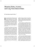
If the economy is suffering a recession and high unemployment, with output below
potential GDP, expansionary monetary policy can help the economy return to potential
GDP. [link] (a) illustrates this situation. This example uses a short-run upward-sloping
Keynesian aggregate supply curve (SRAS). The original equilibrium during a recession
of E0 occurs at an output level of 600. An expansionary monetary policy will reduce
interest rates and stimulate investment and consumption spending, causing the original
aggregate demand curve (AD0) to shift right to AD1, so that the new equilibrium (E1)
occurs at the potential GDP level of 700.

3/10


Monetary Policy and Economic Outcomes

Expansionary or Contractionary Monetary Policy
(a) The economy is originally in a recession with the equilibrium output and price level shown at

E0. Expansionary monetary policy will reduce interest rates and shift aggregate demand to the
right from AD0 to AD1, leading to the new equilibrium (E1) at the potential GDP level of output
with a relatively small rise in the price level. (b) The economy is originally producing above the
potential GDP level of output at the equilibrium E0 and is experiencing pressures for an
inflationary rise in the price level. Contractionary monetary policy will shift aggregate demand
to the left from AD0 to AD1, thus leading to a new equilibrium (E1) at the potential GDP level of
output.

Conversely, if an economy is producing at a quantity of output above its potential GDP,
a contractionary monetary policy can reduce the inflationary pressures for a rising price
level. In [link] (b), the original equilibrium (E0) occurs at an output of 750, which
is above potential GDP. A contractionary monetary policy will raise interest rates,
discourage borrowing for investment and consumption spending, and cause the original
demand curve (AD0) to shift left to AD1, so that the new equilibrium (E1) occurs at the
potential GDP level of 700.
These examples suggest that monetary policy should be countercyclical; that is, it
should act to counterbalance the business cycles of economic downturns and upswings.
Monetary policy should be loosened when a recession has caused unemployment to
increase and tightened when inflation threatens. Of course, countercyclical policy does
pose a danger of overreaction. If loose monetary policy seeking to end a recession goes
too far, it may push aggregate demand so far to the right that it triggers inflation. If tight
monetary policy seeking to reduce inflation goes too far, it may push aggregate demand

4/10


Monetary Policy and Economic Outcomes

so far to the left that a recession begins. [link] (a) summarizes the chain of effects that
connect loose and tight monetary policy to changes in output and the price level.

The Pathways of Monetary Policy
(a) In expansionary monetary policy the central bank causes the supply of money and loanable
funds to increase, which lowers the interest rate, stimulating additional borrowing for
investment and consumption, and shifting aggregate demand right. The result is a higher price
level and, at least in the short run, higher real GDP. (b) In contractionary monetary policy, the
central bank causes the supply of money and credit in the economy to decrease, which raises the
interest rate, discouraging borrowing for investment and consumption, and shifting aggregate
demand left. The result is a lower price level and, at least in the short run, lower real GDP.

Federal Reserve Actions Over Last Four Decades
For the period from the mid-1970s up through the end of 2007, Federal Reserve
monetary policy can largely be summed up by looking at how it targeted the federal
funds interest rate using open market operations.
Of course, telling the story of the U.S. economy since 1975 in terms of Federal Reserve
actions leaves out many other macroeconomic factors that were influencing
unemployment, recession, economic growth, and inflation over this time. The nine
episodes of Federal Reserve action outlined in the sections below also demonstrate that
the central bank should be considered one of the leading actors influencing the macro
economy. As noted earlier, the single person with the greatest power to influence the
U.S. economy is probably the chairperson of the Federal Reserve.
[link] shows how the Federal Reserve has carried out monetary policy by targeting the
federal funds interest rate in the last few decades. The graph shows the federal funds
interest rate (remember, this interest rate is set through open market operations), the
unemployment rate, and the inflation rate since 1975. Different episodes of monetary
policy during this period are indicated in the figure.

5/10

Monetary Policy and Economic Outcomes

Monetary Policy, Unemployment, and Inflation
Through the episodes shown here, the Federal Reserve typically reacted to higher inflation with
a contractionary monetary policy and a higher interest rate, and reacted to higher
unemployment with an expansionary monetary policy and a lower interest rate.

Episode 1
Consider Episode 1 in the late 1970s. The rate of inflation was very high, exceeding 10%
in 1979 and 1980, so the Federal Reserve used tight monetary policy to raise interest
rates, with the federal funds rate rising from 5.5% in 1977 to 16.4% in 1981. By 1983,
inflation was down to 3.2%, but aggregate demand contracted sharply enough that backto-back recessions occurred in 1980 and in 1981–1982, and the unemployment rate rose
from 5.8% in 1979 to 9.7% in 1982.
Episode 2
In Episode 2, when the Federal Reserve was persuaded in the early 1980s that inflation
was declining, the Fed began slashing interest rates to reduce unemployment. The
federal funds interest rate fell from 16.4% in 1981 to 6.8% in 1986. By 1986 or so,
inflation had fallen to about 2% and the unemployment rate had come down to 7%, and
was still falling.
Episode 3
However, in Episode 3 in the late 1980s, inflation appeared to be creeping up again,
rising from 2% in 1986 up toward 5% by 1989. In response, the Federal Reserve used
contractionary monetary policy to raise the federal funds rates from 6.6% in 1987 to

6/10


Monetary Policy and Economic Outcomes

9.2% in 1989. The tighter monetary policy stopped inflation, which fell from above 5%

in 1990 to under 3% in 1992, but it also helped to cause the recession of 1990–1991, and
the unemployment rate rose from 5.3% in 1989 to 7.5% by 1992.
Episode 4
In Episode 4, in the early 1990s, when the Federal Reserve was confident that inflation
was back under control, it reduced interest rates, with the federal funds interest rate
falling from 8.1% in 1990 to 3.5% in 1992. As the economy expanded, the
unemployment rate declined from 7.5% in 1992 to less than 5% by 1997.
Episodes 5 and 6
In Episodes 5 and 6, the Federal Reserve perceived a risk of inflation and raised the
federal funds rate from 3% to 5.8% from 1993 to 1995. Inflation did not rise, and the
period of economic growth during the 1990s continued. Then in 1999 and 2000, the
Fed was concerned that inflation seemed to be creeping up so it raised the federal funds
interest rate from 4.6% in December 1998 to 6.5% in June 2000. By early 2001, inflation
was declining again, but a recession occurred in 2001. Between 2000 and 2002, the
unemployment rate rose from 4.0% to 5.8%.
Episodes 7 and 8
In Episodes 7 and 8, the Federal Reserve conducted a loose monetary policy and slashed
the federal funds rate from 6.2% in 2000 to just 1.7% in 2002, and then again to 1%
in 2003. They actually did this because of fear of Japan-style deflation; this persuaded
them to lower the Fed funds further than they otherwise would have. The recession
ended, but, unemployment rates were slow to decline in the early 2000s. Finally, in
2004, the unemployment rate declined and the Federal Reserve began to raise the federal
funds rate until it reached 5% by 2007.
Episode 9
In Episode 9, as the Great Recession took hold in 2008, the Federal Reserve was quick
to slash interest rates, taking them down to 2% in 2008 and to nearly 0% in 2009. When
the Fed had taken interest rates down to near-zero by December 2008, the economy was
still deep in recession. Open market operations could not make the interest rate turn
negative. The Federal Reserve had to think “outside the box.”

Quantitative Easing
The most powerful and commonly used of the three traditional tools of monetary
policy—open market operations—works by expanding or contracting the money supply

7/10


Monetary Policy and Economic Outcomes

in a way that influences the interest rate. In late 2008, as the U.S. economy struggled
with recession, the Federal Reserve had already reduced the interest rate to nearzero. With the recession still ongoing, the Fed decided to adopt an innovative and
nontraditional policy known as quantitative easing (QE). This is the purchase of longterm government and private mortgage-backed securities by central banks to make
credit available so as to stimulate aggregate demand.
Quantitative easing differed from traditional monetary policy in several key ways.
First, it involved the Fed purchasing long term Treasury bonds, rather than short term
Treasury bills. In 2008, however, it was impossible to stimulate the economy any further
by lowering short term rates because they were already as low as they could get. (Read
the closing Bring it Home feature for more on this.) Therefore, Bernanke sought to lower
long-term rates utilizing quantitative easing.
This leads to a second way QE is different from traditional monetary policy. Instead
of purchasing Treasury securities, the Fed also began purchasing private mortgagebacked securities, something it had never done before. During the financial crisis, which
precipitated the recession, mortgage-backed securities were termed “toxic assets,”
because when the housing market collapsed, no one knew what these securities were
worth, which put the financial institutions which were holding those securities on very
shaky ground. By offering to purchase mortgage-backed securities, the Fed was both
pushing long term interest rates down and also removing possibly “toxic assets” from
the balance sheets of private financial firms, which would strengthen the financial
system.
Quantitative easing (QE) occurred in three episodes:
1. During QE1, which began in November 2008, the Fed purchased $600 billion

in mortgage-backed securities from government enterprises Fannie Mae and
Freddie Mac.
2. In November 2010, the Fed began QE2, in which it purchased $600 billion in
U.S. Treasury bonds.
3. QE3, began in September 2012 when the Fed commenced purchasing $40
billion of additional mortgage-backed securities per month. This amount was
increased in December 2012 to $85 billion per month. The Fed has stated that,
when economic conditions permit, it will begin tapering (or reducing the
monthly purchases). This has not yet happened as of early 2014.
The quantitative easing policies adopted by the Federal Reserve (and by other central
banks around the world) are usually thought of as temporary emergency measures. If
these steps are, indeed, to be temporary, then the Federal Reserve will need to stop
making these additional loans and sell off the financial securities it has accumulated.
The concern is that the process of quantitative easing may prove more difficult to reverse

8/10


Monetary Policy and Economic Outcomes

than it was to enact. The evidence suggests that QE1 was somewhat successful, but that
QE2 and QE3 have been less so.

Key Concepts and Summary
An expansionary (or loose) monetary policy raises the quantity of money and credit
above what it otherwise would have been and reduces interest rates, boosting aggregate
demand, and thus countering recession. A contractionary monetary policy, also called a
tight monetary policy, reduces the quantity of money and credit below what it otherwise
would have been and raises interest rates, seeking to hold down inflation. During the
2008–2009 recession, central banks around the world also used quantitative easing to

expand the supply of credit.

Self-Check Questions
Why does contractionary monetary policy cause interest rates to rise?
Contractionary policy reduces the amount of loanable funds in the economy. As with all
goods, greater scarcity leads a greater price, so the interest rate, or the price of borrowing
money, rises.
Why does expansionary monetary policy causes interest rates to drop?
An increase in the amount of available loanable funds means that there are more people
who want to lend. They, therefore, bid the price of borrowing (the interest rate) down.

Review Questions
How do the expansionary and contractionary monetary policy affect the quantity of
money?
How do tight and loose monetary policy affect interest rates?
How do expansionary, tight, contractionary, and loose monetary policy affect aggregate
demand?
Which kind of monetary policy would you expect in response to high inflation:
expansionary or contractionary? Why?
Explain how to use quantitative easing to stimulate aggregate demand.

9/10


Monetary Policy and Economic Outcomes

Critical Thinking Question
A well-known economic model called the Phillips Curve (discussed in The Keynesian
Perspective chapter) describes the short run tradeoff typically observed between
inflation and unemployment. Based on the discussion of expansionary and

contractionary monetary policy, explain why one of these variables usually falls when
the other rises.

10/10