1.b Valid-Time Indeterminacy in Temporal Relational Databases - Semantics and Representations 2012

IEEE TRANSACTIONS ON KNOWLEDGE AND DATA ENGINEERING, MANUSCRIPT ID

Valid-Time Indeterminacy in Temporal
Relational Databases: Semantics and
Representations
Luca Anselma, Paolo Terenziani, and Richard T. Snodgrass
Abstract—Valid-time indeterminacy is “don’t know when” indeterminacy, coping with cases in which one does not exactly know
when a fact holds in the modeled reality. In this paper, we first propose a reference representation (data model and algebra) in
which all possible temporal scenarios induced by valid-time indeterminacy can be extensionally modeled. We then specify a
family of sixteen more compact representational data models. We demonstrate their correctness with respect to the reference
representation and analyze several properties, including their data expressiveness. Then, we compare these compact models
along several relevant dimensions. Finally, we also extend the reference representation and a representative of compact
representations to cope with probabilities.
Index Terms—H.2.4.m Temporal databases, I.2 Artificial Intelligence, H.2.0.b Database design, modeling and management,
I.2.4 Knowledge Representation Formalisms and Methods.

——————————  ——————————

1 INTRODUCTION

T

attention in the TDB literature.
A commonly agreed-upon strategy to cope with time
in relational databases is to extend the data model to associate temporal elements (i.e., sets of time points, or,
equivalently, sets of time intervals) with tuples, and to
extend relational operators to cope with such an additional temporal component. Specifically, temporal relational operators usually perform “standard” operations
on the non-temporal component, and apply set operators
on temporal elements (e.g., Cartesian product involves
the intersection of the temporal elements of the tuples being paired). However, to the best of our knowledge, such
a methodology has not yet been fully explored in the context of temporal indeterminacy (see the “Temporal Indeterminacy” entry in Liu and Tamer Özsu [19]). For example, the work by Dyreson and Snodgrass [9] only copes

with periods of indeterminacy and does not provide set
operators on them, nor temporal relational operators
working on the extended representation. Additionally, to
the best of our knowledge, no current approach copes
with indeterminacy about existence.
We attempt here to overcome such limitations. Indeed,
our goal is quite ambitious: we do not just aim to provide
a specific representation for indeterminate temporal elements as well as set operators on them (plus the related
temporal relational algebra), but to explore a wide range
of representational possibilities. Indeed, in this paper we
propose 17 different approaches to temporal indeterminacy. We extensively study the main properties of such
————————————————
approaches: (i) expressiveness, (ii) closure and correctness
• L. Anselma is with the Dipartimento di Informatica, Università di Torino, of algebraic operators, and (iii) whether the approaches
Torino, Italy. E-mail:
• P. Terenziani is with the Dipartimento di Informatica, Università del Pie- are a consistent extension of BCDM [14] [20], a semantics
adopted by many temporal database approaches. Finally,
monte Orientale, Alessandria, Italy. E-mail:
we compare such approaches, considering their expres• R.T. Snodgrass is with the Department of Computer Science, University of
siveness, their capability to cope with existential indeter-

ime is pervasive and in many situations the dynamics
over time is one of the most relevant aspects to be
captured by a data model. Many representations for
temporal databases (TDBs) have been developed over the
last two decades.
Valid-time indeterminacy (“don’t know when” information [9]) comes into play whenever the valid time associated with some piece of information in the database is
not known in an exact way. Consider the following example (at a granularity of hours).
Example 1. On Jan 1 2010 between 1am (inclusive) and
4am (exclusive) John had breathing problems.

The fact “John had breathing problems” holds at an
unknown number of time units (hours), ranging from
hours 1 to 3 inclusive, i.e., it may hold on 1, 2, and 3, or on
1 and 3, or on 2 only, and so on. (For the sake of brevity,
in this paper we denote by n the hour from n to n+1, and
we assume to start the numbering of hours on Jan 1 2010).
As a border case, the fact that a given event might have
occurred or not (i.e., indeterminacy about the existence of
the fact) may be interpreted as a form of valid-time indeterminacy; consider:
Example 2. On Jan 1 2010 between 1am (inclusive) and
4am (exclusive) Mary might have had an ischemic stroke.
Coping with valid-time indeterminacy is important in
many database applications, since the time when facts
happen is often partially unknown. However, the treatment of valid-time indeterminacy has not received much

Arizona, Tucson, AZ, USA. E-mail:

Manuscript received on Nov 2 2011.
xxxx-xxxx/0x/$xx.00 © 200x IEEE

1


2

IEEE TRANSACTIONS ON KNOWLEDGE AND DATA ENGINEERING, MANUSCRIPT ID

minacy, their suitability [15], intended as the “intuitive notion of expressiveness which takes the modelling effort
into account” [22], and their computational cost.

1.1 Methodology
In this paper, we ground our approach on BCDM [14]
[20]. We utilize a commonly-used methodology: (1) we
first propose a reference approach coping with the phenomenon; and only then (2) we devise more userfriendly, compact, and efficient representations.
Our reference approach (data model and algebra) allows one to extensionally model (bringing to mind data
expressiveness) and query (query expressiveness) all possible temporal scenarios induced by valid-time indeterminacy. We provide a consistent extension of BCDM, in
the sense that determinate valid time can be easily coped
with as a special case (thus granting for the compatibility
and interoperability with existent approaches). However,
(data/query) expressiveness is not the only criterion. It is
also important to provide users with formalisms that
model phenomena in a “suitable” and “compact” way.
We first identify four refinements (for example, one of
them emphasizes suitability and compactness in coping
with constraints about valid-time minimal duration).
Each refinement is independently satisfied (or not). On
the basis of these refinements, we propose a family of sixteen representations, each supporting a specific combination of such refinements in a more compact and userfriendly way (with respect to the reference approach).
Each representation is characterized (i) by a different
formalism to represent valid time, (ii) by the definition of
set operations (i.e., union, intersection and difference) on
the given representation of valid time, and (iii) by the relational algebra operations based on such set operations.
For each data representation, we study its semantics
and (data) expressiveness with respect to the reference
approach. We have defined the set operators within the
different representations in such a way that they are
proven to be correct with respect to the reference approach. Roughly speaking, this means that, although such
operators operate on a more compact representation, they
provide the same results as the reference approach. However, we proved that not all the sixteen representations
could support a closed definition of set operators: in some
representations, the correct result of set operations cannot

be expressed in the representation formalism. Of course,
only representations which support a closed definition of
set operators —a closed representation for short— are
suitable for DB applications.
For each “closed” representation, we define the relational algebraic operators as a polymorphic adaptation of
the operators of the reference approach and determine
whether each is a consistent extension of the BCDM operators. Finally, we also extend our approach to cope with
probabilities.
This paper thus provides a family of representations of
temporal indeterminacy overcoming the limitations of
current approaches, as well as a formal framework which
can be used in order to analyze and classify extant and
potential representations for valid-time indeterminacy.

Users can choose between such representations the bestsuited approach to model their application domain.
The paper is organized as follows. In Section 2, we present our reference approach. In Section 3, we identify the
four refinements for a compact representation, and we
describe five representations: one for each refinement
plus the representation resulting from the combination of
all the refinements. Section 4 summarizes the results concerning also the other representations in the family. In
Section 5, we extend both the reference approach and one
of the compact representations to deal with probabilities.
Finally, in Section 6 we propose comparisons and in Section 7 we draw some conclusions.

2 REFERENCE APPROACH
In this section, we introduce the reference approach we
propose to cope with temporal indeterminacy. Our starting point is BCDM [14].

2.1 BCDM
BCDM (Bitemporal Conceptual Data Model) [14] is a unifying data model, isolating the “core” semantics underlying many temporal relational approaches, including

TSQL2 [14] [20]. In BCDM, tuples are associated with valid time and transaction time. For both domains, a limited
precision is assumed (the chronon is the basic time unit).
Both time domains are totally ordered and isomorphic to
the subsets of the domain of natural numbers. The domain of valid times DVT is given as a set DVT={c1,…,ck} of
chronons, and the domain of transaction times DTT is given as DTT={c’1,…,c’j}∪{UC} (where UC –Until Changed– is
a distinguished value). In general, the schema of a BCDM
relation R=(A1,...,An|T) consists of an arbitrary number of
non-timestamp (explicit henceforth) attributes A1, …, An,
encoding some fact, and of a timestamp attribute T, with
domain DTT×DVT; the explicit attributes and the
timestamp attribute are separated by the symbol |. Thus,
a tuple x=(v1,…,vn|tb) in a BCDM relation r(R) on the
schema R consists of a number of attribute values associated with a set of bitemporal chronons cbl=(c’h, ci), with
c’h∈DTT and ci∈DVT, to denote that the fact v1,…,vn is current (present in the database) at time c’h and valid at time
ci. An empty timestamp and value-equivalent [20] tuples
are not admitted. Valid-time, transaction-time and atemporal tuples are special cases, in which either the transaction time, or the valid time, or both of them are absent. In
the following, we restrict our attention to valid time (in
fact, temporal indeterminacy cannot affect transaction
time), and extend this general model to deal with temporal indeterminacy.

2.2 Disjunctive temporal elements
As in BCDM [14] (and in many approaches reviewed in
[20]), in our approach time is totally ordered and isomorphic to the natural numbers. For the sake of simplicity, a
single granularity (e.g., hour) is assumed.
Definition 1 Chronon. The chronon is the basic time unit.
The chronon domain TC, also called timeline, is the ordered set of chronons {c1, …, ci, …, cj, …} with ciAs in BCDM, sets of chronons are used in order to as-


ANSELMA ET AL.: VALID-TIME INDETERMINACY IN TEMPORAL RELATIONAL DATABASES: SEMANTICS AND REPRESENTATIONS

sociate with each tuple its valid time.
Definition 2 Temporal element. A temporal element
is a set of chronons, i.e., an element of PS(TC), the power
set of TC.
Disjunctions of temporal elements are a natural way of
coping with valid-time indeterminacy, in which each
temporal element models one of the alternative possible
temporal scenarios (any one of which could be valid).
Definition 3 Disjunctive temporal element, termed
DTE. A disjunctive temporal element is a disjunctive set
of temporal elements. Given a temporal domain TC, a
DTE is an element of PS(PS(TC)).
For example, the following DTE models the valid time
in Example 1: {{1}, {2}, {3}, {1,2}, {1,3}, {2,3}, {1,2,3}}.
Notice that indeterminacy about existence can be
simply modeled by including the empty temporal element within a DTE. Determinate times can be modeled
through a DTE containing just one temporal element
(called singleton DTE).
Property 1 Consistent extension (DTE). Any determinate temporal element can be modeled by a singleton
DTE.

2.2 Temporal tuples and relations
To represent facts that are temporally indeterminate,
DTEs are used as timestamps of the facts. Intuitively,
DTEs cope with valid-time indeterminacy by explicitly
modeling all the alternative temporal scenarios.
Definition 4 (valid-time) indeterminate tuple and relation. Given a schema (A1, …, An) (where each Ai represents a non-temporal attribute on the domain Di), a (valid-time) indeterminate relation r is an instance of the
schema (A1, …, An | VT) defined over the domain
D1 × … × Dn × PS(PS(TC)) in which empty valid times and

value-equivalent tuples are not admitted (as in BCDM).
Each tuple x = (v1, …, vn | d) ∈ r, where d is a DTE, is
termed a (valid-time) indeterminate tuple. The DTE d =
{{ci,…,cj}, …, {ch,…,ck}} within tuple x denotes that the tuple x holds either at each chronon in {ci, …, cj} or … or at
each chronon in {ch, …, ck}.
Example 3. On Jan 1 2010 Sue might have had an ischemic stroke either at 1am or at 2am.
Example 4. On Jan 1 2010 Tim had breathing problems
certainly at 1am and possibly at 2am or 3am.
CLINICAL_RECORD is a temporally indeterminate relation representing Examples 1–4.
CLINICAL_RECORD
{ (John, breath | {{1}, {2}, {3}, {1,2}, {1,3}, {2,3}, {1,2,3}}),
(Mary, stroke | {∅, {1}, {2}, {3}}),
(Sue, stroke | {∅, {1}, {2}}),
(Tim, breath |{{1}, {1,2}, {1,3}, {1,2,3}}) }
The first tuple models Example 1. The second tuple
models Example 2 considering the additional knowledge
that the ischemic stroke, if any, has been unique and has
occurred in –at most– one hour. ∅ represents that the fact
might have not occurred. Finally, the third and fourth tuples model Examples 3 and 4 respectively.

2.3 Lattice of scenarios
The elements of PS(TC) with the standard set inclusion

3

relation form a lattice which represents the space of all
possible alternative scenarios over the temporal domain
TC. We term this a lattice of scenarios (over TC).
Property 2 Expressiveness. By definition, the formalism in this section allows one to express (i.e., to associate
with each tuple) any combination of possible scenarios

(i.e., any subset of the lattice of scenarios).
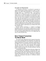
In Figure 1 we represent the lattice of scenarios considering the chronons {1,2,3} and the subsets of the lattice of
scenarios represented by Examples 1, 2 and 3.
In Sections 3 and 4 we describe also less expressive
(but more compact) formalisms, which in some cases
cannot represent all possible combinations of scenarios
(i.e., not all subsets of the lattice of scenarios).

2.4 Algebraic operations
Codd designated as complete any query language that
was as expressive as his set of five relational algebraic operators: relational union (∪), relational difference (–), selection (σP), projection (πX), and Cartesian product (×) [6].
Here we generalize these operators to cover (valid-time)
indeterminate relations. As in several TDB models, our
temporal operators behave as standard non-temporal operators on the non-temporal attributes, and apply set operators on the temporal component of tuples (see, e.g.,
Snodgrass [20]). As in many TDB models, including
TSQL2 and BCDM, in our proposal Cartesian product involves the intersection of the temporal components, projection and union involve their union, and difference the
difference of temporal components. (This definition can
be motivated by a sequenced semantics [8]: results should
be valid independently at each point of time.)
Now we define the relational operators of union (∪TI),
difference (–TI), projection (πXTI), selection (σXTI) and Cartesian product (×TI) between temporally indeterminate
relations. But, before doing so, we define the (generalized) set operators of intersection (∩DTE), union (∪DTE) and
difference (−DTE) applied to DTEs.
Definition 5 ∪DTE, ∩DTE, and −DTE. Given two DTEs DA
and DB, and denoting their temporal elements by A and B
respectively ∪DTE, ∩DTE, −DTE between DA and DB are defined as the DTE obtained through the pairwise application of standard set operations on temporal elements:
DA ∪DTE DB = {A ∪ B | A ∈ DA ∧ B ∈ DB }

{1,2,3}
{1,2}

{1}

{1,3}
{2}
∅

{2,3}
{3}
Ex.3

Ex.1

Ex.2

Figure 1. Lattice of scenarios over the chronons {1,2,3} ordered
with respect to set inclusion. The solid-line oval, the dotted-line
oval and the dashed-line oval represent the scenarios of Example
1, of Example 2 and of Example 3, respectively.


4

IEEE TRANSACTIONS ON KNOWLEDGE AND DATA ENGINEERING, MANUSCRIPT ID

DA ∩DTE DB = {A ∩ B | A ∈ DA ∧ B ∈ DB }
DA −DTE DB = {A − B | A ∈ DA ∧ B ∈ DB }.
Intuitively, DTEs represent valid-time indeterminacy
by eliciting all possible alternative determinate scenarios.
The rationale behind our definition is simply that the
pairwise combination of each alternative scenario must be

taken into account. For instance, considering the CLINICAL_RECORD relation, {∅, {1}, {2}, {3}} ∩DTE {∅, {1}, {2}}
identifies all times when both Mary and Sue had a stroke,
and the final result is the set of scenarios obtained by
combining each scenario for Mary and Sue through pairwise standard set intersection, i.e., {∅∩∅, ∅∩{1}, ∅∩{2},
{1}∩∅, {1}∩{1}, {1}∩{2}, {2}∩∅, {2}∩{1}, {2}∩{2}, {3}∩∅,
{3}∩{1}, {3}∩{2}}, which yields {∅, {1}, {2}}. Hence, it is the
case that (a) there was no time when both Mary and Sue
had a stroke, or (b) they both had a stroke in hour 1, or (c)
they both had a stroke during hour 2.
Definition 6 Temporal relational algebraic operators.
Let r and s denote two (temporal) indeterminate relations
on the proper schema. The temporal algebraic operators
of union, difference, projection, selection and Cartesian
product of r and s are defined as follows.
r ∪TI s = { < v|t > |
∃tr ( < v|tr >∈r ∧ ¬∃ts (< v|ts >∈s) ∧ t = tr )
∨ ∃ts ( < v|ts >∈s ∧ ¬∃tr (< v|tr >∈r) ∧ t = ts )
∨ ( ∃tr ( < v|tr >∈r) ∧ ∃ts ( < v|ts >∈s ) ∧ t = tr ∪DTE ts ) }
r –TI s = { < v|t > |
∃tr ( < v|tr >∈r ∧ ¬∃ts (< v|ts >∈s) ∧ t = tr )
∨ ∃tr ∃ts (< v|tr >∈r ∧ < v|ts >∈s ∧ t = tr –DTE ts ∧
t ≠ {∅} ) }
πXTI(r) = { < v|t > |
∃vr tr (< vr| tr >∈r ∧
DTE
t=
<vr|tr >∈r ∧ v = πX (vr) tr }

∪

v

=

πX(vr))

∧

σPTI(r) = { < v|t > | < v|t >∈r ∧ P(v) }
r ×TI s = { < vr · vs|t> |
∃tr ∃ts ( < vr|tr >∈r ∧ <vs|ts >∈s ∧ t = tr ∩DTE ts ∧ t ≠ {∅}
) }.
In addition to Codd operators, temporal selection can
be added, to select tuples whose valid time t satisfies a
selection condition ϕ. Interestingly, in the case of indeterminate temporal information, one may want to specify
whether the condition ϕ(t) must necessarily (NEC) or
possibly (POSS) hold (three-valued approaches have been
widely used to cope with incomplete information in databases; consider, e.g., Gadia et al. [11]).
σNEC ϕTI(r) = { < v|t > | < v|t >∈r ∧ NEC(ϕ(t)) }
σPOSS ϕTI(r) = { < v|t > | < v|t >∈r ∧ POSS(ϕ(t)) }.
For instance, given the relation CLINICAL_RECORD
and the condition t⊇{1} asking for valid times containing
the chronon 1, σNEC(t⊇{1})TI(CLINICAL_RECORD) = {(Tim,
breath | {{1}, {1,2}, {1,3}, {1,2,3}}) }, while
σPOSS(t⊇{1})TI(CLINICAL_RECORD)
=
CLINICAL_RECORD. We are not committed to any specific
syntax for ϕ. Besides predicates asking for validity at (or
before, or after) specific chronons, we also envision pred-

icates about duration, and about the relative temporal location of tuples (based on Allen’s relations) as in [21].
As the DTE set operators are used in the definition
above, it is useful to consider some nice properties of the
DTE set operators which have bearing on the relational
algebraic operators.
Property 3 Closure of DTE set operators. The representation language of DTEs is closed with respect to the
operations of ∪DTE, ∩DTE and –DTE.
Our approach is a consistent extension of BCDM’s one
(considering valid time only).
Property 4 Consistent extension (DTEs). Determinate
time is represented by singleton DTEs. If only singleton
DTEs are used, the set operators ∪DTE, ∩DTE, and −DTE are
equivalent to the standard set operators ∪, ∩ and −, and
the relational operators ∪TI, –TI, σPTI, σϕt TI, πXTI and ×TI are
equivalent to the standard BCDM valid-time relational
operators ∪t, –t, σPt, σϕt, πXt and ×t.

3 COMPACT REPRESENTATIONS
3.1 General methodology
The above treatment of valid-time indeterminacy is expressive but has several limitations. It is not compact and
thus possibly not suitable [15] nor user-friendly, since all
possible scenarios need to be elicited. More compact (and
possibly more efficient) representations of temporal indeterminacy can be devised, sometimes at the price of losing
part of the data expressiveness of the reference extensional approach. However, the limited expressiveness may be
acceptable in several real-world domains. Instead of proposing a single compact representation, in this paper we
explore (part of) the range of possibilities. Each possibility
is characterized by a different way of representing in a
compact way indeterminate temporal elements. On the
other hand, it is worth stressing that, for all of our representations, we polymorphically apply:
i) the same way of defining tuples and relations;

ii) the same general definition of algebraic relational
operators proposed in Definition 6.
Specifically, given a type X representation of the temporal component we subsequently define (there are several such representations we will consider), we adopt the
following polymorphic definition of tuple and relation, an
extension of Definition 4.
Definition 7 (Valid-time) indeterminate tuple and relation in a compact representation X. Given a schema
(A1, …, An) (where each Ai represents a non-temporal attribute on the domain Di), let VTX be the temporally indeterminate valid time attribute under representation X, let
DX be the domain of VTX, and let a (valid-time) indeterminate relation r for the representation X be an instance
of the schema (A1, …, An | VTX) defined over the domain
D1 × … × Dn × DX in which empty valid times and valueequivalent tuples are not admitted (as in BCDM). Each
tuple x = (v1, …, vn | dX) ∈ r is termed a (valid-time) indeterminate tuple for the representation X. Additionally, in
all the cases, we always adopt the same definition of the
algebraic relational operators (Definition 6), in which the
union, intersection and difference operators between the


ANSELMA ET AL.: VALID-TIME INDETERMINACY IN TEMPORAL RELATIONAL DATABASES: SEMANTICS AND REPRESENTATIONS

temporal components have to be polymorphically instantiated with the specific operators defined for the type X of
the temporal components.
As a consequence, in the following we focus only on
the definition of representation formalisms for temporal
components, and on the definition of intersection, union
and difference set operators on temporal components. For
each representation that we identify, we have adopted a
uniform methodology:
i) we specify its extensional semantics by defining a
function Ext that associates with a temporal component its extensional semantics represented as a
DTE;
ii) we analyze its data expressiveness, both in terms

of the reference approach, and with respect to the
standard determinate approach;
iii) we define the intersection, union and difference
set operators between temporal components, proving their correctness; and
iv) we ascertain the properties of the operators, and of
the induced algebraic operators.
In particular, given a compact representation X, and
given the set operations ∪X, ∩X, and −X on temporal components in X, as regards the data representation formalism (point (ii) above), we verify whether X is a consistent
extension of the determinate temporal model, i.e., if X can
express all the possible determinate temporal components. As regards the set operations, we consider the following properties:
- Closure. The set operations ∪X, ∩X, and −X are closed
(with respect to the representation X) if any application of
the operations on temporal components in X provides as
output a temporal component expressible in X.
- Correctness. Temporal components in a representation X are compact representations of DTEs. Set operators
∪X, ∩X, and −X perform a “symbolic manipulation” on
such representations, providing a compact representation
as a result (i.e., the result is a temporal component in X).
In other words, the result of any set operation T1X OpX T2X
is a temporal component T3X in X which is directly computed only on the basis of the input (i.e., of T1X OpX T2X)
without resorting to their underlying semantics (i.e., to
the DTEs Ext(T1X) and Ext(T2X)). This procedure is efficient, since it only requires a symbolic manipulation on a
compact representation, but demands a proof of correctness. Indeed, we have to prove the correctness of our set
operators with respect to the extensional semantics: the
symbolic manipulation provides the same results (expressed in the representation X) that would be obtained
by operating on the corresponding extensions in the reference approach (i.e., by operating on DTEs). Formally
speaking, we have to prove that, given a compact representation X, and any two temporal components T1X and
T2X in X, we have that:
Ext(T1X ∪X T2X)= Ext(T1X) ∪DTE Ext(T2X)
Ext(T1X ∩X T2X) = Ext(T1X) ∩DTE Ext(T2X)

Ext(T1X –X T2X) = Ext(T1X) –DTE Ext(T2X).
- Consistent extension of set operators. For representations X that are a consistent extension of the determinate temporal model, set operators ∪X, ∩X, and −X are a

consistent extension of the corresponding determinatetime set operators (e.g., of BCDM’s operators ∪t, ∩t, and
−t ) if, in case only temporal components TX’s expressing
determinate temporal components (in the representation
X) are considered, ∪X, ∩X, and −X and ∪t, ∩t, and −t are
equivalent.
- Consistent extension of the indeterminate relations
and of the algebraic operators. Finally, given a compact
representation X, tuples, relations and algebraic operations in X are polymorphically defined on the basis of
temporal components TX and set operations ∪X, ∩X, and
−X in X (see Definition 7). Therefore, from the properties
of consistent extension of the data model and of the set
operators in a representation X, we can always induce
that the relations and algebraic operations in X are a consistent extension of determinate (e.g., BCDM’s) ones.
The range of possible representations has been identified by considering several different refinements. Our
choice has been driven by considerations on expressiveness and usefulness derived from our previous research
experience in both Temporal Databases and Artificial Intelligence, and in many applicative domain, ranging from
medicine to geology. However, in no way do we claim
that the refinements we have identified are the only ones
worth investigating.
We begin with a basic and simple representation, in
which temporal components only consist of independent
indeterminate chronons. This basic representation is then
successively refined into four additional, more expressive
refined representations:
1. Possibility of expressing, besides indeterminate
chronons, also a determinate component;
2. Possibility of coping with non-independent indeterminate chronons (i.e., capability of listing alternative sets of possibilities, possibly excluding

some of the possible combinations);
3. Possibility of expressing a minimum constraint on
the number of chronons;
4. Possibility of expressing a maximum constraint on
the number of chronons.
Refinement 1 is important to model several domains (e.g.,
medicine) in which valid time is usually only partially
unknown. This possibility is present in several models,
both in Artificial Intelligence (consider, e.g., Allen [1]) and
in TDB (e.g., Dyreson and Snodgrass [9]). Refinement 2
derives from the relevance of coping with alternatives in
several domains (e.g., in planning), which is provided by
many approaches, especially in Artificial Intelligence [1].
Refinements 3 and 4 support the treatment of minimal
and maximal durations, as required in many domains
(e.g., medicine).
The rest of this section is organized as follows. First,
Section 3.2 discusses the “basic” compact representation.
Then, in Sections 3.3-3.5, the basic representation is extended to cope with the above possibilities, independently of each other (for the sake of brevity, the possibility of
expressing minimum and maximum constraints is considered together). Finally, in Section 3.6 the combination
of all the different possibilities is taken into account.

5


6

IEEE TRANSACTIONS ON KNOWLEDGE AND DATA ENGINEERING, MANUSCRIPT ID

3.2 Independent indeterminate chronons

In this section we present a compact representation useful
in domains where one can identify a (possibly empty) set
of chronons in which the fact may hold (indeterminate
chronons), and such chronons are independent of each
other, in the sense that all combinations of indeterminate
chronons are possible alternative scenarios. For instance,
consider the following.
Example 5. On Jan 1 2010 Ann might have had breathing problems between 1am (inclusive) and 4am (exclusive).
Here the fact may not hold, or it may hold in each of
the hours 1, 2, and 3, considered independently of each
other (meaning that it may hold at ∅, {1}, {2}, {3}, {1,2},
{1,3}, {2,3}, {1,2,3}). In this section, we show that valid
times of this type can be modeled by a representation
formalism that is (strictly) less data expressive than the
formalism of DTEs, yet supports a more compact and user-friendly representation.
Definition 9 Indeterminate temporal element, termed
ITE. An ITE <i> is represented by a temporal element, i.e.,
i ⊆ TC.
The extensional semantics of such a representation can
be formalized taking advantage of the reference approach
in Section 2.
Definition 10 Extensional semantics of ITEs. The semantics of an ITE <i> is the DTE consisting of all and only
the combinations of the chronons in i, i.e., Ext(<i>)= PS(i).
Example 5 can be represented by the indeterminate
temporal element {1,2,3}, and its underlying semantics is
the DTE Ext(<{1,2,3}>) = {∅, {1}, {2}, {3}, {1,2}, {1,3}, {2,3},
{1,2,3}}. 1
ITEs are less expressive than DTEs, since not all combinations of temporal scenarios can be expressed.
Property 5 Expressiveness of ITE. Given a temporal
domain TC, ITEs allow one to express all and only the elements of PS(PS(TC)) of the form PS(INDET), where INDET ⊆ TC.

Intuitively, the formalism only allows one to cope with
those subsets of TC in which all the possible combinations
of indeterminate chronons are present. For instance, Example 3 is not expressible, since there is a dependency between the indeterminate chronons 1 and 2, which are mutually exclusive.
We now define the set operators on ITEs. In one sense,
we have already done so, in Definition 5. However, that
definition is in terms of the extension, whereas we would
like to operate directly at the level of the representation,
which is a succinct characterization of a set of scenarios,
as expressed by the extension.
It turns out that the set operators are quite natural to
express directly in the ITE representation.
Definition 11 Set operators ∪ITE, ∩ITE, and –ITE on
ITEs. Given two ITEs <i> and <i’>,
<i> ∪ITE <i’> = < i∪i’>
<i> ∩ITE <i’> = < i∩i’>
1 Notice that, for the sake of efficiency, contiguous sets of chronons in
each temporal element can be compactly represented by the periods covering them (e.g., {{1,2,3,4,6,7,8}, {8,9,10}} can be equivalently represented
by {{[1-4],[6-8]},{[8-10]}}).

<i> –ITE <i’> = <i>.
The union (intersection) of two ITEs is the ITE resulting from the union (intersection) of the sets of the chronons in the ITEs. Interestingly, the difference between
two ITEs is the minuend. Specifically, the chronons in the
ITEs are only possible, not definite, so that the chronons in
the subtrahend may not exist, and so, they must not be
subtracted from the indeterminate chronons in the minuend.
ITE tuples and relations can be polymorphically defined as shown by Definition 7. In particular, an ITE tuple
is a non-temporal tuple paired with an ITE, and an ITE
relation is a set of non-value equivalent ITE tuples. To define the relational temporal algebraic operators on ITE relations, we polymorphically adopt the definition of relational algebraic temporal operators of the extensional semantics (see Definition 6), in which the set operators ∪DTE,
∩DTE and –DTE on DTEs are substituted by the set operators ∪ITE, ∩ITE and –ITE on ITEs.
Property 6. Properties of the ITE representation. ITE

set operators are closed and correct. No consistent extension property holds in ITE.
Proof. Correctness of intersection (∩ITE):
Since, by definition, <i> ∩ITE <i’> = < i∩i’>, we have to
prove that Ext(<i>) ∩DTE Ext(<i’>) = Ext(< i∩i’>). By the
semantics of ITEs, Ext(<i>)=PS(i) and, by the definition of
intersection between DTEs and by the distributive law of
intersection over power sets, Ext(<i>) ∩DTE Ext(<i’>) =
PS(i) ∩DTE PS(i’) = { a ∩ b | a∈PS(i) and b∈PS(i’) } =
PS(i∩i’) = Ext(<i∩i’>). 
As regards the consistent extension property, let us
consider the DTE {{1}}, containing just the determinatetime temporal element {1}: it is not possible to model it
with an ITE because the extension of any ITE necessarily
contains also the empty temporal element ∅.
A drawback of ITEs is that they represent only indeterminate chronons. Thus, ITEs cannot represent determinate time. An ITE can represent that Ann might have
had breathing problems between 1am and 4am (Example
5), but not that Ann definitely had breathing problems at
5am. This limitation implies that ITE relations are not a
consistent extension of BCDM, and ITE relational operators are not a consistent extension of BCDM operators.
However, such properties will hold for the representation
to be described in the following Section.

3.3 Determinate chronons
In this section we present a compact representation
useful in domains where, besides independent indeterminate chronons, one can identify a (possibly empty) set
of chronons in which the fact certainly holds (termed determinate chronons). For instance, consider Example 4 in
Section 2.2.Valid times of this type can be modeled by a
representation formalism that is (strictly) less data expressive than the formalism of DTEs, yet supports a more
compact and user-friendly representation.
Definition 12 Determinate+Indeterminate temporal
element, termed DITE. A DITE is a pair <d,i>, where d

and i are temporal elements.
Intuitively, the first element of the pair identifies the


ANSELMA ET AL.: VALID-TIME INDETERMINACY IN TEMPORAL RELATIONAL DATABASES: SEMANTICS AND REPRESENTATIONS

determinate chronons, and the second element the indeterminate ones. The extensional semantics of such a representation can be formalized taking advantage of the
general approach in Section 2.
Definition 13 Extensional semantics of DITEs. The
semantics of a DITE <d,i> is the DTE consisting of all and
only the sets that contain d and the combinations of the
chronons in i, i.e., Ext(<d,i>) = { d ∪ e | e ⊆ i }.
Example 4
can be represented by the determinate+indeterminate temporal element <{1},{2,3}>, and its
underlying semantics is the DTE Ext(<{1},{2,3}>) = {{1},
{1,2}, {1,3}, {1,2,3}}.
DITEs are less expressive than DTEs, since not all
combinations of temporal scenarios can be expressed.
Definition 14 Set operators ∪DITE, ∩DITE, and –DITE.
Given two DITEs <d,i> and <d’,i’>,
<d,i> ∪DITE <d’,i’> = <d∪d’, i∪i’>
<d,i> ∩DITE <d’,i’> = <d∩d’, (d∪i) ∩ (d’∪i’)>
<d,i> –DITE <d’,i’> = <d – (d’∪i’), (d∪i) – d’>. ■
Property 7. Properties of the DITE representation.
DITE set operators are closed and correct. The consistent
extension properties hold in DITE.
A detailed treatment of DITEs, of the related algebra
and of its properties is reported in the preliminary version of this work in [2].

3.4 Dependent indeterminate chronons

Coping with non-independent indeterminate chronons
involves the necessity of preventing some combinations
of indeterminate chronons from being included in the extensional semantics of the temporal components. Consider Example 3, where not all the combinations of the chronons are allowed because hours 1 and 2 are mutually exclusive. In this section, we augment the basic representation (which only considers independent indeterminate
chronons) to model also dependent indeterminate chronons and we describe a representation formalism that is
(strictly) less data expressive than the formalism of DTEs,
yet more compact and user friendly.
Definition 15 Dependent Indeterminate temporal element, termed DeITE. A DeITE is a set {i1, …, in}, where
each ij is a temporal element, i.e., ij ⊆ TC.
Intuitively, the semantics of a DeITE is the union of the
semantics of the ITEs i1, …, in.
Definition 16 Extensional semantics of DeITEs. The
semantics of a DeITE {i1, …, in} is the DTE consisting of all
and only the sets that contain the combinations of the
chronons in each ij, i.e., Ext({i1, …, in}) = { e | e⊆i1 ∨ … ∨
e⊆in }.
Example 3 can be represented by the dependent indeterminate temporal element {{1},{2}} and its underlying
semantics is the DTE Ext({{1},{2}}) = {∅, {1}, {2}}.
DeITEs are less expressive than DTEs, since not all
combinations of temporal scenarios can be expressed.
Property 8 Expressiveness of DeITE. Given a temporal domain TC, DeITEs allow one to express all and only the subsets of PS(PS(TC)) of the form PS(INDET1) ∪ …
∪ PS(INDETn), where INDETj ⊆ TC, j=1, …, n.
This property states that DeITEs are less expressive
than DTEs, since not all combinations of temporal scenar-

ios can be expressed. For instance, Example 1 cannot be
expressed with a DeITE: in fact John certainly had breathing problems, so that the empty temporal element ∅ must
not be in the extensional semantics of the DeITE, but with
a DeITE it is not possible to exclude ∅.
Definition 17 Set operators ∪DeITE, ∩DeITE, and –DeITE.
Given two DeITEs {i1, …, in} and {i’1, …, i’h},

{i1, …, in} ∪DeITE {i’1, …, i’h} = {ij ∪ i’k | 1≤j≤n, 1≤k≤h}
{i1, …, in} ∩DeITE {i’1, …, i’h} = {ij ∩ i’k | 1≤j≤n, 1≤k≤h}
{i1, …, in} –DeITE {i’1, …, i’h} = {i1, …, in}.
The union, intersection and difference between two
DeITEs is the pairwise union, intersection and difference
of the ITEs that compose the DeITEs (see the definition of
∪ITE, ∩ITE, and –ITE).
The following properties hold for DeITE:
Property 9. Properties of the DeITE representation.
DeITE set operators are closed and correct. No consistent
extension property holds in DeITE.
As regards consistent extension, since ITEs are a special case of DeITEs with one component, the same counterexample provided for ITEs is applicable here.

3.5 Minimum and maximum cardinality
Minimum and maximum cardinality constraints are useful in order to explicitly model constraints about temporal
duration. For instance, the constraint that ischemic stroke
happened in at most one hour (see Example 2) can be
stated by setting the maximum cardinality constraint to 1.
In this section, we augment the basic representation
with independent indeterminate chronons to model minimum and maximum constraints on the components.
Definition 18 Independent Indeterminate temporal
element with minimum/maximum constraints, termed
mMITE. An mMITE is a triple <i, m, M>, where i is a
temporal element, m and M are non-negative integers,
specifying the minimum and maximum cardinalities, respectively, with m≤M.
Definition 19 Extensional semantics of mMITEs. The
semantics of an mMITE <i, m, M> is the DTE consisting of
all and only the combinations of the chronons in i with
cardinality between m and M, i.e., Ext(<i, m, M>) = { e |
e⊆i ∧ m ≤ |e| ≤ M }.

Consider the following example.
Example 6. On Jan 1 2010 between 2am (inclusive) and
5am (exclusive) Sue had breathing problems for two
hours within that three-hour period.
Example 6 can be compactly represented by the
mMITE <{2,3,4},2,2>, and its underlying semantics is the
DTE Ext(<{2,3,4},2,2>) = {{2,3}, {2,4}, {3,4}}.
mMITEs are less expressive than DTEs, since not all
combinations of temporal scenarios can be expressed.
Property 10 Expressiveness of mMITE. Given a temporal domain TC, a subset INDET of TC and two nonnegative integers m and M with m≤M, mMITEs allow one
to express all and only the subsets of PS(PS(TC)) of the
form PS(INDET), whose cardinalities are between m and
M.
Example 4 cannot be represented with a mMITE: in
fact, if the component i of the mMITE has to contain the
chronons 1, 2 and 3 (since Tim had breathing problems in

7


8

IEEE TRANSACTIONS ON KNOWLEDGE AND DATA ENGINEERING, MANUSCRIPT ID

such hours) and if the extension of the mMITE has to contain the chronon 1 alone, it must also contain all the other
temporal elements with cardinality 1 (i.e., the chronons 2
and 3 alone), while they are not possible.
Unfortunately, this representation is not closed with
regard to the set operators and, thus, also the relative relational algebra is not closed. For instance, we show that
the difference set operator is not closed. In order to be

correct, the mMITE difference set operator should satisfy:
Ext(<i, m, M> –mMITE <i’, m’, M’>) = Ext(<i, m, M>) –DTE
Ext(<i’, m’, M’>).
Let us consider <{1, 2, 3},1,3> –mMITE <{2,3},1,2>. If the
difference is defined correctly (with respect to the reference approach), the result of the above operation must be
Ext(<{1, 2, 3},1,3>) –DTE Ext({2,3},1,2>) = {∅, {1}, {2}, {3},
{1,2}, {1,3}}. However, this DTE is not expressible by an
mMITE; in fact, the temporal element of cardinality 2 {2,3}
is missing (see Property 10).

3.6 Combinations
We have explored all possible combinations of the
above refinements (indeed, we have also considered the
minimum and the maximum constraints as independent
refinements, to be combined with the other ones). For the
sake of brevity, in this section we only consider the representation that includes all the refinements: determinate
and indeterminate chronons, dependent indeterminate
chronons, and minimum and maximum cardinality. A
systematic analysis of all the representations we explored
is given in the next section.
Definition 20 Determinate+Dependent Indeterminate temporal element with minimum/maximum cardinality, termed mMDDeITE. An mMDDeITE is a pair {<i1,m1,M1>, …, <in,mn,Mn>}>, where d is a temporal element, and for j=1, …, n ij are temporal elements, mj and
Mj are non-negative integers, and mj≤Mj.
Definition 21 Extensional semantics of mMDDeITEs.
The semantics of a mMDDeITE <in,mn,Mn>}> is the DTE consisting of all and only the sets
that contain the chronons in d and the combinations of the
chronons in each ij that satisfy the cardinality constraint,
i.e., Ext(∧ m1≤|e|≤M1) ∨ … ∨ (e⊆in ∧ mn≤|e|≤Mn) }.

Consider the following example.
Example 7. On Jan 1 2010 Ann-Marie had breathing
problems at 1am, and then either for 1–2 hours between
3am (inclusive) and 6am (exclusive) or for 1–2 hours between 8am (inclusive) and 10am (exclusive).
Example 7 can be represented by the mMDDeITE <{1},
{<{3,4,5},1,2>, <{8,9},1,2>}> and its underlying semantics
is the DTE Ext(<{1}, {<{3,4,5},1,2>, <{8,9},1,2>}>) = {{1,3},
{1,4}, {1,5}, {1,3,4}, {1,3,5}, {1,4,5}, {1,8}, {1,9}, {1,8,9}}.
mMDDeITEs are as expressive as DTEs, thus all combinations of temporal scenarios can be expressed.
Property 11 Expressiveness of mMDDeITE. Given a
temporal domain TC, mMDDeITEs allow one to express
all and only the subsets of PS(PS(TC)).
In other words, mMDDeITEs have the same expressiveness of DTEs, that is, of the full extension. Intuitively,
given a DTE dte = {{ch1, …, chk}, …, {ci1, …, cil}}, it is possible

to define a mMDDeITE having dte as an extension by setting each first component ij (j=1, …, n) of the triplets mj, Mj> of the mMDDeITE to one of the elements of dte,
i.e., the mMDDeITE corresponding to dte is <∅, {<{ch1, …,
chk},k,k>, …, <{ci1, …, cil},l,l>}>.
Determinate valid time can be easily captured by
means of mMDDeITEs.
At this point, the set operations of union (∪mMDDeITE),
intersection (∩mMDDeITE) and difference (−mMDDeITE) between mMDDeITEs can be defined.
Definition 22 ∪mMDDeITE, ∩mMDDeITE, and –mMDDeITE.
Given two mMDDeITEs and {<i1,m1,M1>,
…,
<in,mn,Mn>}>

∪mMDDeITE

mk≤|b|≤Mk | j=1, …, n, k=1, …, h }>
{<i1,m1,M1>,
…,
<in,mn,Mn>}>
∩mMDDeITE
{<(d∪a)∩(d’∪b), |(d∪a)∩(d’∪b)|, |(d∪a)∩(d’∪b)|> | a⊆ij,
b⊆i’k | mj≤|a|≤Mj, mk≤|b|≤Mk | j=1, …, n, k=1, …, h } >
…,
<in,mn,Mn>}>
–mMDDeITE
{<i1,m1,M1>,
∪ i’h), { <(d∪a) – (d’∪b), |(d∪a) – (d’∪b)|, |(d∪a) –
(d’∪b)|> | a⊆ij, b⊆i’k | mj≤|a|≤Mj, mk≤|b|≤Mk | j=1, …,
n, k=1, …, h}>.
The definition of the mMDDeITE operators generalizes
the operators described in the previous sections. The determinate component of the output is evaluated as for the
DITE [2] (obviously, for the determinate component of
the difference, we exclude all the ITEs in the indeterminate component of the subtrahend).
For the indeterminate component, we consider the
subsets a⊆ij, b⊆i’k of the input indeterminate components
that satisfy the minimum and maximum constraints, and

we perform pairwise union, intersection and difference
(see the definition of the DeITE operators in Section 3.4)
by considering also the determinate component (see the
definition of the DITE operators in Section 3.2). The minimum/maximum cardinalities are the cardinalities of the
resulting sets.
Property 12. Properties of the mMDDeITE representation. mMDDeITE set operators are closed and correct.
The consistent extension properties hold in mMDDeITE.

4 COMPARISON OF THE REPRESENTATIONS
Since the four refinements pointed out in Section 3.1 are
orthogonal, implying that all possible combinations are
feasible, in our overall approach we have identified sixteen different languages to express valid-time indeterminacy, plus the extensional one discussed in Section 2. We
have considered five out of the sixteen languages in Sections 3.2–3.6. In this section, we provide a general overview of the whole family of representations, analyzing
and comparing them.
Notation. In the following, we use short tags to denote
the refinements and, then, the seventeen formalisms. RA
denotes the reference approach introduced in Section 2. I


ANSELMA ET AL.: VALID-TIME INDETERMINACY IN TEMPORAL RELATIONAL DATABASES: SEMANTICS AND REPRESENTATIONS

denotes the treatment of indeterminate chronons, and
D+I the treatment of both determinate and indeterminate
chronons. Superscript * denotes the possibility of specifying multiple alternatives concerning the indeterminate
temporal element (i.e., of coping with non-independent
indeterminate chronons). Finally, superscripts n and N
denote the possibility of expressing minimality and maximality constraints respectively. Combinations of tags
represent combinations of refinements.
The seventeen languages thus are RA, I, D+I, I*, D+I*,
In, D+In, In,*, D+In,*, IN, D+IN, IN,*, D+IN,*, In,N, D+In,N, In,N,*,

and D+In,N,*. Specifically, I, D+I, I*, In,N, D+In,N,* correspond
to the representations discussed through Sections 3.2–3.6.
In the following, we discuss important properties that
some of the languages share.

4.1 Closure
The first, fundamental property we consider is closure. In
fact, if the temporal representation is not closed with respect to the set operators of union, intersection and difference, the relational algebra itself (defined in Section
2.4) is not closed. Hence, representations for which closure does not hold are not suitable in the DB context.
Property 13 Closure. The formalisms RA, I, D+I, I*, In,*,
D+In,*, IN,*, D+IN,*, In,N,*, D+In,N,* are closed with respect to
set operators, while the formalisms D+I*, In, D+In, IN,
D+IN, In,N, D+In,N are not.
We have shown in Section 3.5 that In,N is not closed. In
general, we can see that the addition of the minimal
and/or maximal constraint, if it is not paired with the
possibility of specifying multiple alternatives concerning
the indeterminate temporal element (* symbol), leads to
representation languages that are not closed, independently of whether the treatment of determinate chronons is considered. Intuitively, this is because, considering the lattice of scenarios introduced in Section 2.3, In, IN ,
In,N, D+In, D+IN, D+In,N can represent the entire part of the
lattice from which we possibly exclude a bottom part (because of the minimum cardinality) and/or a top part (because of the maximum cardinality). However, the difference between two mMITEs can generate a region not definable by simply cutting away a bottom or top part of the
lattice (see the counterexample in Section 3.5).
Moreover, it is interesting to notice that, even though
the language D+I, described in Section 3.3, is closed, adding the possibility of listing alternatives concerning indeterminate chronons (i.e., the language D+I*) results in a
language that is not closed. For example, consider the set
operator of difference and the operation in D+I* <{1,2},
∅> – <∅, {{1}, {2}}>. The extensional semantics of the result is the DTE {{1}, {2}, {1,2}}, which is not expressible in
D+I* since it has an empty determinate component (because the temporal elements have no common chronon),
but the empty temporal element is not present (and a DeITE cannot exclude ∅ when the determinate component is
empty).

In the remainder of this section, we further investigate
the properties of the closed representations.

9

RA
In,N,*

D+In,N,*
D+In,*

D+IN,*

In,*

IN,*
I*

D+I
I

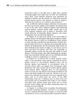
Figure 2. Graphical representation of the data expressiveness of the nine closed representations for expressing validtime indeterminacy studied in our work (as well as the reference approach, RA).

4.2 Expressiveness
Considering the closed representations, we compare their
expressiveness in Figure 2. In this figure, the representations are denoted as rectangles. Solid arcs connect a less
expressive to a more expressive language. Dotted arcs
connect languages with equal expressiveness. The dashed
arc connects two incomparable languages. The relations
derivable by transitive closure are not represented.

We have proven that four of the nine closed representations are as expressive as the reference approach RA.
Property 14 Expressiveness. The representations
D+In,*, D+In,N,*, In,*, In,N,* are as expressive as RA. I, D+I, I*,
IN,*, D+IN,* are less expressive than RA.
In general, the possibility of setting a minimum constraint, in addition to the possibility of specifying multiple alternatives concerning the indeterminate temporal
element (i.e., * plus n), renders a language as expressive
as RA i.e., such that any DTE X can be represented by the
formalisms. Intuitively, this is because through the alternative refinement (* feature) one can elicit all temporal
elements in X. In principle, the extensional semantics of
each alternative is not just one temporal element, but the
power set of the chronons it contains. However, by imposing for each alternative the constraint that the minimum constraint must be exactly the number of chronons
in that alternative, just all and only the sets that are the
temporal elements in X are considered.
Thus, D+In,*, D+In,N,*, In,*, In,N,* can express (possibly in
a more compact way) all the possible combinations of alternative scenarios.
It is interesting to notice how the expressiveness
changes as we add refinements to a language. For example, starting from the D+I representation, if we add the
possibility of expressing alternatives concerning the indeterminate component, we derive the representation D+I*,
which is not closed, as commented above. However, if we
add to D+I the possibility of expressing both alternatives
concerning the indeterminate component and minimality
constraints (refinements (2) and (3) in Section 3.1), we obtain a closed language, D+In,*, which is strictly more expressive, and that is as expressive as RA. If we add to


10

IEEE TRANSACTIONS ON KNOWLEDGE AND DATA ENGINEERING, MANUSCRIPT ID

D+I* the possibility to express maximality constraints (obtaining D+IN,*), we obtain a closed language, with different expressive power. In fact, D+IN,* cannot express arbitrary DTEs since all extensions have to include either the
empty temporal element (since the determinate component is empty) or a same temporal element (since the determinate component is not empty).

On the other hand, starting from the I* representation,
if we add the possibility of expressing minimality constraints, we augment its expressivity resulting in a representation that is as expressive as RA (see the discussion
above); however, if we add to I* the possibility of expressing maximality constraints, the expressivity of the representation does not change. Indeed, given a set of chronons with maximum cardinality N, it can be equivalently
represented by alternative sets of chronons. For instance,
a set {1,2,3} with maximum cardinality 2 (whose extension
is {∅, {1}, {2}, {3}, {1,2}, {1,3}, {2,3}}) may be represented by
the DeITE {{1,2}, {1,3}, {2,3}}.
An asymmetry in Figure 2 can be observed in that the
expressiveness of D+I cannot be compared with I*. For
example, on the one hand the DTE {∅, {2}, {3}} can be expressed by I* as the set {{2},{3}} containing two alternatives, but cannot be expressed by D+I, because, since the
empty temporal element is present, the determinate component must be empty, but including the chronons 2 and
3 in the indeterminate component would necessarily include also the temporal element {2,3}. On the other hand,
we cannot conclude that I* is more expressive than D+I,
because, for example, the DTE {{2}, {2,3}} is expressible by
D+I as <{2},{3}>, but cannot be expressed by I* because it
does not contain the empty temporal element, which is
necessarily contained in every DTE generated by I*.

4.3 Consistent extension
The property of consistent extension (of BCDM) is also
important, to grant for the compatibility and interoperability with existent BCDM-based representations.
Property 15 Consistent extension. The representations
D+I, D+In,*, D+IN,*, D+In,N,*, In,*, In,N,*, and RA are a consistent extension of BCDM. I, I*, IN,* are not.
Of course, all the representations that have a determinate component are trivially a consistent extension of
BCDM, since the determinate component models determinate BCDM times. And, trivially, RA models determinate time through singleton DTEs. Moreover, it is worth
noticing that, while the representation I (i.e., independent
indeterminate chronons, discussed in Section 3.2) is not a
consistent extension, the addition of the possibility of expressing alternatives (*) and minimality constraint (n) to it
grants the property. This is because—as discussed
above—In,* is as expressive as RA and thus it can model

determinate time as RA does. On the other hand, I* and
IN,* are not consistent extensions of BCDM because they
can represent only DTEs where the empty temporal element is necessarily present.

4.4 Existential indeterminacy
Another relevant property about expressiveness regards
how the different representations cope with the indeter-

minacy about the existence of a given tuple (termed existential indeterminacy). All the representations allow to state
that the fact described by the tuple may also not occur
(notice that this fact can be represented in RA by including the empty set in the DTE; additionally, the empty set
is necessarily included in the extensions of every ITE). On
the other hand, not all the representations allow one to
model the fact that there is no existential indeterminacy,
i.e., that the tuple certainly exists (although we might not
know exactly when).
Property 16 Existential indeterminacy. All the representations can represent existential indeterminacy. On the
other hand, I, I*, and IN,* cannot represent certainty of existence.
Of course, certainty of existence can be trivially represented by all representations that support determinate
chronons. Similarly, the representations that do not provide certainty of existence cannot represent determinate
time and, thus, are not consistent extensions of BCDM.
Additionally, the possibility of specifying a minimum
cardinality allows one to express certainty of existence,
since the minimum cardinality allows one to exclude the
empty set from the extensions.

4.5 Compactness and suitability (base relations)
Finally, it is worth stressing that expressiveness is not the
only criterion worth to be considered when evaluating
representations (otherwise RA could suffice). Compactness is also important, as is suitability [15]. For instance,

consider Example 4: it can be expressed in a more compact way in D+I than in In,N,*, even though D+I is strictly
less expressive than In,N,*. In fact, on the one hand in D+I
it can be expressed —as described in Section 3.3— as
<{1},{2,3}>. On the other hand, in In,N,* it can be expressed
as the set of alternatives { <{1},1,1>, <{1,2},2,2>,
<{1,3},2,2>, <{1,2,3},3,3> }, containing four alternatives.
As another example, consider:
Example 8. On Jan 1 2010 Tom might have had fever
between 1am (inclusive) and 4am (exclusive) for at most 2
hours.
This example can be expressed in a more compact way
in IN,* than in D+In,*, even though IN,* is strictly less expressive than D+In,*. In fact, in IN,* it can be expressed as
{<{1,2,3},2>}, while in D+In,* it can be expressed as <∅,
{<{1,2},0>, <{1,3},0>, <{2,3},0>}>.

4.6 Evaluation of set operators
Until now we have considered, besides closure (which is
required for making queries possible), properties related
to the expressiveness of the representations, and their capability to cope with certain phenomena (possibly, in a
suitable way). However, such properties have a cost, both
in terms of the storage needed to represent (temporal) data, and in term of the (temporal) complexity of performing algebraic operators. Note that in order to have the closure property the minimum and/or maximum cardinality
refinements cannot come alone, but require that also the
“*” (multiple alternatives) refinement is provided.
Several factors can be considered to characterize the
“cost” of refinements. In the following, we consider the


ANSELMA ET AL.: VALID-TIME INDETERMINACY IN TEMPORAL RELATIONAL DATABASES: SEMANTICS AND REPRESENTATIONS

length of the output of set operators on the different types

of temporal components, which, besides storage requirements, also gives an insight about the complexity needed
to evaluate algebraic operations. The evaluation of set operators (and thus of algebraic operators) for the representations I and D+I (i.e., for ITEs and DITEs) simply involves union, intersection and difference on sets of chronons, and the length of the output is linear with respect to
the length of the input. The introduction of the “*” refinement demands for a pairwise combination of the input alternatives for the evaluation of set operators, implying that the length of the output may be quadratic with
respect to the length of the input. The introduction of the
cardinality refinements further increases the complexity:
by definition, all the subsets satisfying the cardinality
constraints of the input sets of chronons must be taken
into account. Thus, the output may grow exponentially
with respect to the length of the input.

4.7 Summary
To wrap up, Table 1 compares along various aspects considered in this paper the ten representations that are
closed with regard to set operators. The first four columns
show the four refinements we identified in Section 3.1.
Each column states whether it is possible to express a
phenomenon in a compact/user-friendly way (e.g., RA
allows one to express the minimal duration constraint,
but only eliciting all possible cases; thus RA does not exhibit such a property). Det stands for the possibility of expressing determinate chronons, Dep for coping with dependent chronons, Min and Max for the possibility of expressing minimum and maximum constraints respectively. The fifth column focuses on the possibility of coping
with certainty of existence; the sixth column takes into
account expressiveness (only the representations that
have the full expressiveness of RA are marked); the seventh column considers the consistent extension property 2;
Finally, the eighth column represents the cost of each representation X, considering the length of the output of set
operators with respect to the length of their input (as expressed in the representation X). Considering cost, it is
worth noticing that (i) RA is the most “costly” approach
(even if its output is at most quadratic with respect to the
input). This is due to the fact that the representations (of
the input and of the output) are not compact: all the scenarios are explicitly represented. Thus, for instance, the
evaluation of union must consider all possible pairs of
scenarios, which is the upper bound for the complexity
for all the representations (provided that they are correct

with respect to RA), and (ii) all set operators of representations considering the “D” refinement have been defined
in such a way that, if only determinate chronons are used,
no additional cost is incurred with respect to standard
approaches to determinate time.

2 In Table 1, Cert exist and Consist Ext coincide. However, this is not a
general rule. For instance, a formalism providing for enumerators such as
“one_of” or “at_least_one” associated with temporal elements allows one
to express certainty of existence, but it is not a consistent extension of
BCDM (since purely determinate time cannot be represented).

11

TABLE 1.
COMPARISON OF THE TEN APPROACHES.
Det Dep Min Max

Cert Full Consist
exist Expr
Ext

I

Size
outp
lin

I*

X

In,*

X

IN,*

X

In,N,*

X

X

X

X

D+I

X

D+In,*

X

D+IN,*

quad

X

X

X

X

exp

X

X

X

exp

X

lin

X

X

exp

X
X

exp
X

X

X

D+In,N,* X

X

RA

X

X

X
X

X

X

exp

X

X

X

X

exp

X

X

X

quad

5 PROBABILISTIC EXTENSION
In some approaches in the literature, temporal indeterminacy has been dealt with in conjunction to probabilities
[9] [7]. Intuitively, probabilities, when available, provide
additional pieces of information for discriminating between alternative scenarios. In the following, we sketch
how our approach can be extended to cope with probabilities. We operate in two steps. First, we extend the reference approach to cope with probabilities. Then, we move
towards compact representations. In particular, we only
consider the formalism for independent indeterminate
chronons (Section 3.2). The same methodology can be
used to extend also the other representations. However,
several challenging issues have to be taken into account,
left for future work.

5.1 Probabilistic Reference approach
We assume that facts in the database are independent,
and that for each fact temporal scenarios are exhaustive

and mutually exclusive. For each fact in the database, we
introduce a probability distribution function P, which
gives the probability that the fact occurred in a scenario
(i.e., in a temporal element associated with the fact).
Definition 23 Probabilistic disjunctive temporal element, termed PDTE. A probabilistic disjunctive temporal
element is a disjunctive S set of temporal elements associated with a probability distribution function
P: S  [0,1].
Notation. For the sake of simplicity, we annotate each
temporal element with its probability and we term it as
probabilistic temporal element.
Example 9. (Sue, stroke | {∅0.4, {1}0.1, {2}0.4, {1,2}0.1}) represents the fact that on Jan 1 2010 Sue might have had an
ischemic stroke either at 1am (with probability 0.1) or at
2am (with probability 0.4) or from 1am to 2am included
(with probability 0.1) or might not (with probability 0.4).
As we did for DTEs, we define the (generalized) set
operators of intersection, union and difference applied to
PDTEs.
Definition 24 ∪PDTE, ∩PDTE, and −PDTE. Given two
PDTEs DA and DB, and denoting their probabilistic temporal elements by Ap and Bp’ respectively, the operations


12

IEEE TRANSACTIONS ON KNOWLEDGE AND DATA ENGINEERING, MANUSCRIPT ID

OpPDTE of union (∪PDTE), intersection (∩PDTE), and difference (−PDTE) between DA and DB are defined as the PDTE
obtained through the pairwise application of standard set
operations Op on A and B; the probability is the product
p*p’ of the probabilities of Ap and Bp’. In the case that more
than one pair of probabilistic temporal elements Ap and

Bp’ gives rise to the same probabilistic temporal element
Cp’’, we sum all their products p*p’:
DA OpPDTE DB = {Cp’’ | ∃Ap∈DA ∃Bp’∈DB (C=A Op B) ∧
p’’=Σ p
p*p’}.
p’
A ∈DA ∧ B ∈DB ∧ C=(A Op B)

Example 10. {∅0.4, {1}0.1, {2}0.4, {1,2}0.1} ∩PDTE {∅0.3, {2}0.2,
{3}0.3, {2,3}0.2} = {∅0.8, {2}0.2}.

5.2 Probabilistic independent indeterminate
chronons
In the compact representation IP, as in I, we associate a set
of chronons with a tuple. Since, as in I, there is no explicit
representation of scenarios, in IP we associate probabilities with each chronon.
Definition 25 Probabilistic indeterminate temporal
element, termed PITE. A PITE <i> is represented by a
temporal element, i.e., i ⊆ TC, and a probability function
PI: i  (0,1].
Notice that, for the sake of compactness, we do not
admit chronons with null probability in PITEs.
Notation. When there is ambiguity, we use the notation PIi(c) to represent the probability of the chronon c in
the PITE <i>.
Example 11. <10.2, 20.5> represents that the fact holds in
the hour 1am with probability 0.2, and in the hour 2am
with probability 0.5. Notice that probabilities in a PITE do
not necessarily sum up to 1, since they represent marginal
probabilities with respect to the probabilities of the corresponding PDTEs (see Definition 26 below).
Definition 26 Extensional semantics of PITEs (ExtP

function). The semantics of a PITE =<c1p1, …, ckpk> is the
PDTE consisting of all and only the probabilistic temporal
elements resulting from the combinations of the chronons
in {c1, …, ck}; the probability of a probabilistic temporal
element is the product of the probabilities that each chronon is or is not in the scenario, i.e.,
ExtP(<c1p1, …, ckpk>) = {{ci, …, cj}p | {ci, …, cj}⊆{c1, …, ck}
∧ p= p’1*…*p’k, where p’l=pl if cl∈{ci, …, cj}, p’l=(1–pl) if
cl∉{ci, …, cj}.
Example 12. ExtP(<10.2, 20.5>)={∅0.4, {1}0.1, {2}0.4, {1,2}0.1},
i.e., <10.2, 20.5> is the compact PITE representation of the
PDTE in Example 9 above.
For the sake of simplicity, in the following formulas we
assume that, given a PITE i, if c∉i then PIi(c)=0.
Definition 27 Set operators ∪PITE, ∩PITE, and –PITE on
PITEs. Given two PITEs <i1> and <i2>,
<i1> ∪PITE <i2> = <{cp | (c∈i1 ∨ c∈i2) ∧ p=PIi1(c)*PIi2(c)
+ PIi1(c)*(1–PIi2(c)) + (1–PIi1(c))*PIi2(c)}>
<i1> ∩PITE <i2> = <{cp | c∈i1 ∧ c∈i2 ∧ p=PIi1(c)*PIi2(c)}>
<i1> –PITE <i2> = <{cp | c∈i1 ∧ p=PIi1(c)*(1–PIi2(c)) ∧
p≠0}>.
For intersection, we compute the set intersection of the
chronons; the probability of each chronon in the result is
the product of the input probabilities of the chronon in
each set. For union, we compute the set union of the

chronons; the probability of each chronon in the result is
the sum of the probabilities that the chronon is in both the
sets i1 and i2 or only in the set i1 or only in the set i2. For
difference, the result is the minuend; the probability of
each chronon is the probability that the chronon is in the

minuend and is not in the subtrahend. If a chronon has
null probability, it is not included in the result.
Example 13. <10.2, 20.5> ∩PITE <20.4, 30.5> = <20.2>. Notice
that ExtP(<20.4, 30.5>)={∅0.3, {2}0.2, {3}0.3, {2,3}0.2}, and
ExtP(<20.2>) = {∅0.8, {2}0.2}, so that the above PITE intersection corresponds to the PDTE intersection in Example 10
(and is, indeed, correct).
The following property grants that the direct operations on PITEs are closed and correct with respect to the
probabilistic reference approach PDTE. Notice that IP is a
consistent extension of BCDM since determinate chronons can be represented by associating them with the
probability 1.
Property 17. Properties of the PITE representation.
PITE set operators are closed and correct. PITE is a consistent extension of BCDM.
Proof. Correctness of intersection (∩PITE):
We have to prove that ExtP(<i1> ∩PITE <i2>) = ExtP (<i1>)
PDTE
ExtP(<i2>).
∩
The definition of ∩PITE consists of two parts, the former
defining the output chronons, and the latter defining their
probabilities. The first part of the definition is exactly the
same as for ITEs, so that its proof of correctness has been
already given. Let i1=<{c1p1, …, clpl, c’1p’1, …, c’mp’m}> and
i2=<{c1q1, …, clql, c’’1q’’1, …, c’’nq’’n}>, where i1 and i2 have the
common chronons c1, …, cl. We thus have that <{c1p1, …,
clpl, c’1p’1, …, c’mp’m}> ∩PITE <{c1q1, …, clql, c’’1q’1, …, c’’nq’n}> =
<{c1r1, …, clrl}> is correct for some probability values r1, …,
rl. Now we have just to prove that r1=p1*q1, …, rl=pl*ql.
Let us consider an arbitrary chronon cj∈{c1, …, cl}.
First we notice that, for the semantics of IP (see the definition of ExtP), PIi(cj) is the marginal probability of cj in
the probability distribution P of ExtP(<i>), i.e.,

PIi(cj)= ΣKp∈ExtP(<i>) | cj∈K p.
Let DCcj∈(ExtP(<i1>) ∩PDTE ExtP(<i2>)) be the subset of
ExtP(<i1>) ∩PDTE ExtP(<i2>) which contains only the probabilistic temporal elements including the chronon cj. Let
DCcj = { C1s1, …, Coso}. Then, for the definition of intersection ∩PDTE, each C1s1, …, Coso is the intersection between a
probabilistic temporal element Ap of ExtP(<i1>) which contains cj and a probabilistic temporal element Bp’ of
ExtP(<i2>) which contains cj (i.e., DCcj = {Cp’’ |
∃Ap∈ExtP(<i1>), ∃Bp’∈ExtP(<i2>) (cj∈A ∧ cj∈B ∧ C=A∩B) ∧
p’’=ΣAp∈ExtP(<i1>) ∧ Bp’∈ExtP(<i2>) ∧ cj∈A ∧ cj∈B ∧ C=A∩B p*p’}).
Thus, the probability rj of the chronon cj is the marginal probability of cj, i.e., rj = ΣCp∈DCcj p = ((1–p1)*…*pj*…*(1–
pl)*(1–p’1)*…*(1–p’m)) * ((1–q1)*…*qj*…*(1–ql)*(1–q’1)*…*(1–
+
…
+
(p1*…*pj*…*pl*p’1*…*p’m)
*
q’n))
(q1*…*qj*…*ql*q’1*…*q’n) = pj*qj. 

6 RELATED WORK
In general, temporal logics have been extensively used for
representing and reasoning about propositions and predicates whose truth depends on time. These systems are


ANSELMA ET AL.: VALID-TIME INDETERMINACY IN TEMPORAL RELATIONAL DATABASES: SEMANTICS AND REPRESENTATIONS

usually developed around a set of temporal connectives,
such as sometimes/always in the future, until etc. that provide implicit reference to time instants. First-order temporal
logic is a variant of temporal logic that allows first-order
predicate symbols, variables and quantifiers, in addition
to connectives. Many temporal logics have been proposed, differing in terms of expressiveness, order, time

metric, temporal modalities, time model, and time structure (see, e.g., the survey in Emerson [10]). In the area of
databases, some of such logics have been used as temporal
query languages for timestamped temporal data (see, e.g.,
the survey by Chomicki and Toman – “Temporal Logic in
Database Query Languages” entry in Liu and Tamer
Özsu [19]).
Probabilistic temporal logics have been developed to reason about dynamic systems which include uncertainty
and probabilistic assumptions. Both classical and nonclassical logics have been extended to cope with probabilities. For instance, PCTL extends the branching time temporal logic CTL and is interpreted over discrete-time
Markov chains; PTCTL extends the real-time branching
logic TCTL, PDC extends the duration calculus DC; PNL
extends the Neighbourhood Logic; Generalised Probabilistic Logic (GPL) is a Mu-calculus-based modal logic (references to these and other logics can be found in the recent survey by Konur [16]).
One of the earliest efforts to incorporate probabilistic
information within a relational database is due to Cavallo
and Pittarelli [4], who also proposed a partial relational
algebra for the extended model. Probabilistic approaches
have been widely used to cope with probabilistic temporal data and temporal indeterminacy (see, e.g., the recent survey “Probabilistic Temporal Databases” entry in
Liu and Tamer Özsu [19]). For instance, Dekhtyar et al. [7]
introduce temporal probabilistic tuples to cope with data
such as “data tuple d is in relation r at some point of time
in the interval [ti,tj] with probability between p and p’.“
They also provide algebraic relational operators for their
data model. However, they restrict their attention to
events that are instantaneous, while our approach also
considers events with duration (indeed, the minimum
and maximum duration constraints would be meaningless with instantaneous events only). Another influent
probabilistic approach to temporal indeterminacy has
been proposed by Dyreson and Snodgrass [9]. Here, valid-time indeterminacy is coped with by associating a period of indeterminacy with a tuple. A period of indeterminacy is a period between two indeterminate instants,
each one consisting of a range of chronons and of a probability distribution over it. Since the ranges of chronons
defining the starting and ending points of a period cannot
overlap, periods of indeterminacy must have at least one

“determinate” chronon. Thus, indeterminacy about existence cannot be expressed, and, disregarding probabilities,
Snodgrass and Dyreson’s approach is strictly enclosed in
our D+I representation as regards expressiveness.
In the line of Artificial Intelligence research, Brusoni et
al. [3] and Koubarakis [17] independently proposed a different approach, addressing indeterminacy in the context
of temporal constraints between tuples, with specific at-

tention to relative times.
Finally, it is worth mentioning that, indeed, temporal
indeterminacy is just a specific case of incomplete information. Many approaches have been developed to cope
with incomplete information in relational databases (see,
e.g., the extensive bibliography in Lipski [18] as regards
early works, and Grahne [12]). For instance, Imielinski
and Lipski [13] have identified precise conditions that
should be satisfied by usual algebraic relational operators
to meaningfully cope with relations where various kinds
of “null values” are allowed. Gadia [11], e.g., provided a
“bridge” between works on incomplete information and
temporal relational databases. Interestingly, Gadia introduced partial temporal elements (and set operators on them)
to cope with temporally indeterminate information, that
closely resemble our DITEs (and set operators on DITEs).
Also, Gadia et al. cope with values whose occurrence is
uncertain, thus considering a form of what we term existential indeterminacy.

7 CONCLUSIONS
Though temporal indeterminacy is inherent in many realworld domains, it has received relatively limited attention
within the database literature. In particular, the identification and analysis of different representations and of set
operators for indeterminate temporal elements has not
been adequately explored within the specialized literature. In this paper, we address this limitation. We identify
a spectrum of approaches (data models, each with set operators and relational algebraic operators) to treat validtime indeterminacy, and analyze their properties and

their suitability to model phenomena in a compact way.
The incorporation of a refinement into a representation
may improve not only the expressiveness of the representation, but also its compactness and suitability, thus possibly making it more “natural” to use. Therefore, among
suitable representations, D+In,N,* seems to be the best
choice if one wants to reconcile the full data expressiveness of RA with compactness, since D+In,N,* supports a
determinate component, temporal dependence and cardinality constraints in a compact way. However, refinements have their own cost, especially in terms of the
evaluation of set operations on temporal components.
Therefore, we think that there is no “best representation”
per se: the main contribution of Table 1 is to indicate users and developers the representation “best suited” to
model the specific application they work with. For example, in case a user needs to compactly express determinate
chronons, but she does not need to cope with either nonindependent indeterminate chronons, or cardinality constraints, Table 1 shows that, for that particular situation,
the D+I representation is the “best suited” one. This
choice of the “best suited” representation might be done
by the DB administrator, on the basis of the specific domain/application. Specifically, we envision the development of a user-friendly interface to help administrators in
this choice (e.g., by exemplifying the choice criteria summarized in Table 1). Indeed, the “best suited” representation could also be chosen at a finer granularity, i.e., on a

13


14

IEEE TRANSACTIONS ON KNOWLEDGE AND DATA ENGINEERING, MANUSCRIPT ID

per-tuple basis. In such a context, additional operators
must be provided to convert representations as needed
based on their relative expressiveness. This is a goal of
our future work.
Also, the lattice in Figure 2 can be used as a framework
to analyze the expressiveness of current and (possibly)
future representations in the literature.

As future work, we wish also to extend our approach
to consider other refinements besides the ones described
in Section 4. A practically relevant issue is convexity since
in many domains indeterminacy at chronon c is correlated with indeterminacy near c. For instance, for convex
ITEs, Ext(<{2,3,4}>) could be {∅, {2}, {3}, {4}, {2,3}, {3,4},
{2,3,4}} (thus excluding {2,4} which is not convex). However, the problem of providing a semantically correct definition of set operators for such representations requires
further investigations. Additionally, a task of our future
work is to extend also the other compact representations
to cope with probabilities, applying the methodology of
Section 5. Finally, our long-term goal is the development
of suitable extensions to the SQL standard to treat the different forms of indeterminacy considered in this paper.

[12]
[13]
[14]
[15]

[16]
[17]

[18]

[19]
[20]
[21]

ACKNOWLEDGMENT
This work was supported in part by NSF grants IIS0803229 and IIS-1016205. The authors are grateful to the
anonymous reviewers for their constructive comments.

REFERENCES
[1]

J. F. Allen, Time and time again: The many ways to represent time. Int.
J. Intell. Syst., 6, pp. 341–355, 1991.
[2] L. Anselma, P. Terenziani and R.T. Snodgrass. Valid-Time Indeterminacy in Temporal Relational Databases: A Family of Data Models.
Proc. of 17th International Symposium on Temporal Representation and
Reasoning (TIME'10), pp. 139-145, 2010.
[3] V. Brusoni, L. Console, P. Terenziani, B. Pernici, Qualitative and Quantitative Temporal Constraints and Relational Databases: Theory, Architecture, and Applications. IEEE Trans. On Knowledge and Data Engineering 11(6), pp. 948-968, 1999.
[4] R. Cavallo, M. Pittarelli. The Theory of Probabilistic Databases. VLDB,
71-81, 1987.
[5] J. Clifford, C. Dyreson, T. Isakowitz, C.S. Jensen, and R.T. Snodgrass,
On the semantics of “now” in databases. ACM Transactions on Database
Systems, 22(2), 171-214, 1997.
[6] E. F. Codd, Relational Completeness of Data Base Sublanguages. In: R.
Rustin (ed.), Database Systems 65-98, Prentice Hall and IBM Research
Report RJ 987, San Jose, California, 1972.
[7] A. Dekhtyar, R. Ross, and V.S. Subrahmanian. Probabilistic temporal
databases, I: algebra. ACM Transactions on Database Systems, 26(1), pp.
41-95, 2001.
[8] J. Dunn, S. Davey, A. Descour, and R.T. Snodgrass, Sequenced Subset
Operators: Definition and Implementation, proc. ICDE'02, 2002.
[9] C. E. Dyreson and R. T. Snodgrass, “Supporting Valid-time Indeterminacy”, ACM Transactions on Database Systems, 23(1), pp. 1-57, 1998.
[10] A. E. Emerson, Temporal and Modal Logic, In: Van Leeuwen (ed)
Handbook of Theoretical Computer Science, Vol. B, pp. 997-1072, Elsevier Science Publishers, 1990.
[11] S.K. Gadia, S.S. Nair, and Y.-C. Poon. “Incomplete Information in Relational Temporal Databases,” in Proceedings of the International Con-

[22]

ference on Very Large Databases, Vancouver, Canada, pp. 395-406,

1992.
G. Grahne. The problem of incomplete information in relational databases. LNCS 554. Springer Verlag, 1991.
T. Imieliński and W. Lipski, Jr.. 1984. Incomplete Information in Relational Databases. J. ACM 31, 4, 761-791, 1984.
C. S. Jensen and R. T. Snodgrass, “Semantics of Time-Varying Information”, Information Systems, 21(4), 311–352, 1996.
B. Kiepuszewski, “Expressiveness and Suitability of Languages for
Control Flow Modelling in Workflows”. PhD thesis, Queensland University of Technology, Brisbane, Australia, 2003.
S. Konur, Real-time and probabilistic temporal logics: An overview.
Cornell University Library (May 2010), />M. Koubarakis. Representation and Querying in Temporal Databases:
The Power of Temporal Constraints. In Proc. International Conf. on Data Engineering, pp. 327-334, 1993.
W. Lipski. Logical problems related to temporal information in databases. Tech. Rep. 138, Laboratoire de Recherche en Informatique, Université de Paris-Sud, Centre d’Orsay, 1983.
L. Liu, M. Tamer Özsu (Eds.): Encyclopedia of Database Systems.
Springer US 2009.
R.T. Snodgrass (ed), The TSQL2 Temporal Query Language, Kluwer, 1995.
P. Terenziani, R.T. Snodgrass. Reconciling Point-based and Intervalbased Semantics in Temporal Relational Databases: A Proper Treatment of the Telic/Atelic Distinction. IEEE TKDE 16(4), 540-551, 2004.
W.M.P. van der Aalst, “Pi Calculus Versus Petri Nets. Let us eat ‘humble pie’ rather than further inflate ‘Pi hype’”. BPTrends 3(5):1-11, 2005.

Luca Anselma received his PhD in Computer Science from Università di Torino in 2006. He is an assistant professor in Computer Science at the Università di Torino, Italy. His main research interests are
in the areas of Temporal Reasoning, Temporal Databases, Modelbased Diagnosis and Medical Informatics. He is the author of more
than 30 papers in international journals, books and international refereed conferences.
Paolo Terenziani received his Laurea degree in 1987 and his PhD
in computer science in 1993 from Università di Torino, Italy. He is full
professor in computer science with DiSIT, Institute of Computer Science, Università del Piemonte Orientale “Amedeo Avogadro”, Alessandria, Italy. His research interests include artificial intelligence
(knowledge representation and temporal reasoning), databases and
computer science in medicine. He has published more than 100 papers on these topics in refereed journals and conference proceedings.
Richard T. Snodgrass joined the University of Arizona in 1989,
where he is a Professor of Computer Science. He holds a B.A. degree in Physics from Carleton College and M.S. and Ph.D. degrees
in Computer Science from Carnegie Mellon University. He is an
ACM Fellow. Richard's research foci are ergalics, compliant databases, and temporal databases.
Richard was Editor-in-Chief of the ACM Transactions on Database
Systems from 2001 to 2007, was ACM SIGMOD Chair from 1997 to

2001, and has chaired the ACM Publications Board, the ACM History
Committee, and the ACM SIG Governing Board Portal Committee.
He served on the editorial boards of the International Journal on Very
Large Databases and the IEEE Transactions on Knowledge and Data Engineering. He chaired the Americas program committee for the
2001 International Conference on Very Large Databases and the
program committee for the 1994 ACM SIGMOD Conference. He received the 2004 Outstanding Contribution to ACM Award and the
2002 ACM SIGMOD Contributions Award.
He chaired the TSQL2 Language Design Committee and edited the
book, "The TSQL2 Temporal Query Language." He co-directs TimeCenter, an international center for the support of temporal database
applications on traditional and emerging DBMS technologies. He
currently is a member of the Advisory Board of ACM SIGMOD and
chairs the Outstanding Contribution to ACM Award Committee.