DSpace at VNU: A Novel Behavior-based Navigation Architecture of Mobile Robot in Unknown Environments

VNU Journal of Science: Mathematics – Physics, Vol. 32, No. 3 (2016) 19-33

A Novel Behavior-based Navigation Architecture of Mobile
Robot in Unknown Environments
Nguyen Thi Thanh Van*, Phung Manh Duong, Dang Anh Viet, Tran Quang Vinh
VNU University of Engineering and Technology, Hanoi, Vietnam
Received 08 September 2016
Revised 20 September 2016; Accepted 30 September 2016

Abstract: This study proposes behavior-based navigation architecture, named BBFM, for mobile
robot in unknown environment with obstacles. The architecture is carried out in three steps: (i)
analyzing the navigation problem to determine parameters of the architecture; (ii) designing the
objective functions to relate input data with the desired output; and (iii) fusing the output of each
objective function to generate the optimal control signal. We use fuzzy logic to design the
objective functions and multi-objective optimization to find the Pareto optimal solution for the
fusion. A number of simulations, comparisons, and experiments were conducted. The results show
that the proposed architecture outperforms some popular behavior- based architectures in
navigating the mobile robot in complex environments.
Keywords: Behavior-based navigation, fuzzy logic, multi-objective optimization, mobile robot.

1. Introduction
Navigation is fundamental for mobile robot applications. In order to complete any given task, the
robot first needs to have capability to safely reach the target [1]. Navigation of mobile robots thus has
been receiving much research attention. The exiting methods can be classified into two main
categories: hierarchical architectures and reactive or behavior-based architectures [2]. The
hierarchical architecture operates through sequent steps of sensing, planning and acting based on
known model of the environment. This architecture is thus appropriate for static and structured
environments. For unknown or unstructured environments, the behavior-based architecture is often
used. This approach splits a complex navigation task into sub-tasks or behaviors. Each behavior has its
own objective and executes independently. They are then combined in accordance to the state of
environment to generate a global response. As the combination only uses the local data, the behaviorbased architecture does not need to have a global map of the environment. The division into behaviors

additionally enables the modularization and extendability of the architecture.
The main challenge with the behavior-based architecture is the combination of behaviors, called
command fusion, to achieve the navigation objective. Several techniques have been proposed such as
switching [3], motor schema [4], and decentralized information filter (DIF) [5]. However, the most

_______


Corresponding author. Tel.: 84-912720780
Email:

19


20

N.T.T. Van et al. / VNU Journal of Science: Mathematics – Physics, Vol. 32, No. 3 (2016) 19-33

popular one is the fuzzy-based technique, which was practically used in recent mobile robot
navigation systems [6-10]. In this technique, each behavior is presented by one fuzzy controller. The
command fusion is then the fusion of output fuzzy sets of controllers and the final control signal is the
value of defuzzification. This technique is simple in implementation and quite efficient in navigation.
The command fusion, however, is not optimal due to limitation of defuzzification methods [11], [12].
Each method often results in a different value of defuzzification. These values, in some cases, even
conflict with each other.
In order to deal with the optimization problem in command fusion, a technique based on multiobjective optimization theory, called MOASM, was proposed [13]. This technique represents each
behavior by an objective function that relates input parameters such as mechanical structure, kinematic
model and environment dynamics with the degree of achievement of the control objective. These
functions are then combined using the multi-objective optimization to find an optimal solution which
maximizes them. However, the main drawback of this technique is the lack of process for designing

the objective functions. These functions may so complicated that preventing the technique to be
deployed in practice.
In this study, we propose a behavior-based navigation architecture, called BBFM, which
inherits advantages of fuzzy logic to design the objective functions and multiobjective optimization to
fuse the behaviors. In BBFM, each behavior is represented by a reduced fuzzy controller which only
contains the fuzzification and fuzzy inference processes. As the result, the output of each fuzzy
controller will be a function of input variables whose value presents the achievement of behavior
objective, or in other words, the objective function. These functions thus can be used as inputs for a
multi objective optimization process to find the optimal control signal. A number of simulations,
comparisons, and experiments have been carried out and the results confirmed the efficiency of the
proposed architecture in navigating the mobile robot in complex and unknown environments.
The structure of paper includes six sections. Section II presents the BBMF architecture in
general. Section III describes the implementation of BBFM for the case of differential drive wheeled
mobile robot. Section IV simulates and compares the BBFM with two other popular architectures. The
experimental results are presented in Section V. The paper finishes with discussions and conclusions
in Section VI.
2. Behavior-Based Navigation and the BBFM Architecture
In this section, we present two popular fusion tech- niques. One uses fuzzy logic and the other uses
multiple objectives optimization. Based on them, the BBFM architecture is proposed.
A. Behavior-based navigation using fuzzy logic
In behavior-based navigation using fuzzy logic, each behavior is implemented by a fuzzy
controller. Each fuzzy controller includes three modules: fuzzification, inference engine and command
fusion. The fuzzification describes data via linguistic values, for example the distance is near or far,
without requiring the system model so that it is suitable for uncertainty characteristics of unknown
environment. The fuzzy inference is executed by ”If...Then” rules similarly to the human’s inference.
Finally, command fusion generates the overall control signal in one of two ways shown in Fig.1:
defuzzicating first and then combining individual decisions; or combining individual decisions first
and then defuzzicating.

N.T.T. Van et al. / VNU Journal of Science: Mathematics – Physics, Vol. 32, No. 3 (2016) 19-33

21

Fig. 1. Two approaches to command fusion: (a) Defuzzificating and then combining,
(b) Combining and then defuzzificating.

Advantages of behavior-based navigation using fuzzy logic includes the ease in implementation
and efficiency in navigation. However, the command fusion is not optimal. Fig.1 shows that the two
ways of command fusion give different results. In addition, defuzzification methods such as centroid,
mean of maximum or last of maximum produce different values. Consequently, the efficiency of
navigation is not stable. In practice, we realize that the global control signal generated in some
situations may even conflict with the output signal of certain behaviors.
B. Behavior-based navigation using multi-objective optimization
In behavior-based navigation using multi-objective optimization, each behavior is described by
an objective function Ok (y) , where y  ( y1 , y2 ,..., yn ) Y is the vector of control signal and Y is a set
of possible actions, or control parameters. The optimal overall control signal is the solution of
following equation:

yˆ  max[O1 (y), O2 (y),, ON (y)].

(1)

According to the theory of multi-objective optimization, there does not exist the optimal solution,

yˆ , of Equation (1), but only the ”good enough” solution, y* , which is the best fit to all objectives Oi.
*
This solution is called the Pareto optimal solution or non-dominated solution defining as follows: y
is the Pareto optimal solution of Equation (1) if there does not exist any y Y such that
Oi (y)  Oi (y* ) at least one i and Oj (y)  Oj (y* ) for all j. In other words, the Pareto optimal solution is

the one in which there is not other solution that improves an objective without resulting in the
deterioration of at least one other objective. Popular methods used to find the Pareto optimal solution
includes the weighting, lexicographic and goal programming [14].
It is recognizable that the theory of multi-objective optimization provides a method to find the
optimal solution for command fusion. However, it does not supply the method for defining objective
functions. Without it, the deployment of this technique in practice is limited as the objective functions
varies between systems and are often complex to manually define.
C. Behavior-based navigation architecture - BBFM
From the analyses, we realize that it is possible to inherit advantages of fuzzy logic and multiobjective optimization by using the output membership functions of fuzzy controllers as the objective
functions for multiobjective optimization because each membership function maps the input space to
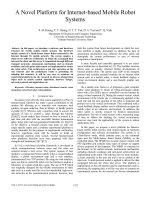
the interval of [0, 1] representing the achievement of behavior objective. Fig. 2 shows the block
diagram of BBFM. Each fuzzy controller is employed to build an objective function. The command
fusion module then combines all objective functions using multi-objective optimization to generate the
overall control signal. The deployment of BBFM is carried out in three steps: task analysis, objective
function design, and command fusion. Details of each step are described as follows.


22

N.T.T. Van et al. / VNU Journal of Science: Mathematics – Physics, Vol. 32, No. 3 (2016) 19-33

Fig. 2. The block diagram of BBFM architecture.

1) Task analysis
The purpose of task analysis is to determine main parameters for the BBFM architecture including
the number of behaviors, their objectives, and the dimension of control signal. The number and
objectives of behaviors are located based on the robot configuration, operating environment, and task
assigned. The dimension of control signal depends on robot configuration and control method.
Typically, outputs of all behavior need to have the same dimension to ensure the feasibility of
command fusion: dim(yi )  dim(y j ) .

2) Objective function design
Based on the parameters, a fuzzy controller is built for each behavior. It includes the fuzzification
and fuzzy inference processes. The defuzzification is ignored. Consequently, the output of each fuzzy
controller is a membership function which can be used as the objective function for the command
fusion. Details of implementation are described as follows.
* Fuzzification
Fuzzification defines the input/output linguistic variables and their fuzzy sets. For each fuzzy
controller, it is necessary to determine m input linguistic variables {x1, x2… xm} with the universe of
discourse {X1, X2… Xm} and n output linguistic variables {y1, y2..., yn} with the universe of discourse {Y1,
Y2… Yn}. Each input linguistic variable represents data from an input such as the distance measured by
an ultrasonic sensor. Each output linguistic variable on the other hand represents a component of the
control signal such as the tangent velocity. Values of a linguistic variable are determined by the fuzzy
sets. Denoting a fuzzy set as Aij, the input linguistic variable xi and output linguistic variable yi are then
represented by:

x1  {A11 , A12 ,, A1a }
x2  {A21 , A22 ,, A2a }
...
xm  {Am1 , Am2 ,, Ama }
y1  {B11 , B12 ,, B1b }
y2  {B21 , B22 ,, B2b }
...
yn  {Bn1 , Bn 2 ,, Bnb }

(2)


N.T.T. Van et al. / VNU Journal of Science: Mathematics – Physics, Vol. 32, No. 3 (2016) 19-33

23

The membership functions are then represented by:

x1 : ( A11 ( x1 ),  A12 ( x1 ),,  A1a ( x1 ))
x2 : ( A21 ( x2 ),  A22 ( x2 ),,  A2 a ( x2 )
...
xm : ( Am1 ( xm ),  Am 2 ( xm ),,  Ama ( xm ))
y1 : (B11 ( y1 ), B12 ( y1 ),, B1b ( y1 ))

(3)

y2 : (B21 ( y2 ), B22 ( y2 ),, B2b ( y2 ))
...
yn : (Bn1 ( yn ), Bn 2 ( yn ),, Bnb ( yn ))
where Aij is the membership function of input variables, Bij is the membership function of
output variables.
* Fuzzy Inference
Fuzzy inference is the process of building control rules and combining them to make output
fuzzy sets. Each control rule, Rk, is of the form ”If...then...”, for instance:
If x1 = A11 and x2 = A21 and . . . xm = Am1 then y1 = B11 and y2 = B21 and . . . yn = Bn1.
The result of above rule for each output control signal yi is determined by:

R ( y1 )  min( H , B ( y1 ))
R ( y2 )  min( H , B ( y2 ))
k

11

k

21

...

(4)

R ( yn )  min( H , B ( yn ))
H  min{ A ( x1 ),  A ( x2 ),,  A ( xm )}
k

n1

11

21

m1

For M control rules, the implication R’ of each yi according to the max-min method is an output
fuzzy set with the membership function defined by:

R ( yi )  max(R ( yi ), R ( yi ),, R ( yi )), ON (y)]
1

2

M

(5)

The membership function (5) is the objective function of control signal yi.
3) Command fusion
The command fusion generates a overall control signal by fusing outputs of all fuzzy controllers.
Let N be the number of fuzzy controllers. Each component, yi, of the control signal then has N
objective functions determined by (5). According to multi-objective optimization theory, the Pareto
optimal solution, yˆi , has to satisfy the following condition:

µ
yi  max[R1 ( yi ), R2 ( yi ),, RN ( yi )]

(6)

It can be found by using the Lexicographic method [14] as follows:
 Sorting all behaviors in descending order of importance, for example behavior 1, behavior
2, ..., behavior N.
 Sequentially solving equations Pi until an unique solution is obtained or all equations are
solved:


24

N.T.T. Van et al. / VNU Journal of Science: Mathematics – Physics, Vol. 32, No. 3 (2016) 19-33

P1 : max R1 ( yi ),
yi Yi

P2 : max R2 ( yi ),
yi Yi1

...

Pj : max Rj ( yi ),

(7)

yi Yi ( j 1)

Yj ( j 1)  {yi | yi is the solution of Pj 1},
j  2,, N  1
3. Implementation of BBFM for Differential Drive Wheeled Mobile Robot
This section presents the deployment of BBFM architecture for the differential drive wheeled
mobile robot in unknown environments. Details of the steps of task analysis, objective function design
and command fusion are described as follows.
A. Task analysis
This step determines parameters of the BBFM architecture based on the configuration of robot and
task assigned.
1. Robot configuration
The robot is the type of differential drive wheeled mobile robot with nonholonomic constraints and
parameters shown in Fig. 3, where (OG, XG, YG) is the global coordinate system; (OR, XR, YR) is the
local coordinate system relative to the robot chassis; R is the wheel diameter; L is the distance between
two wheels; (x, y, θ) represents the position and the direction of robot in the global coordinate system;
ρ is the distance from the center of robot to the target; α is the angle between the axis of the robot’s
reference frame and the vector connecting the center of the axle of the wheels with the target position.
The kinematic equation in discrete time domain of the robot is presented by [15]:

xi 1  xi  uiTs cosi

 yi 1  yi  uiTs sini
     T .
i s
 i 1 i

(8)

where Ts is the sampling period, ui and ωi are respectively the tangential and angular velocity at
sampling time i.
YR

YG

XR

Target
α

ρ

YR

XR

u

ω

θ
OR

L

OG

R

XG

Fig. 3. Configuration of the differential drive wheeled mobile robot.


N.T.T. Van et al. / VNU Journal of Science: Mathematics – Physics, Vol. 32, No. 3 (2016) 19-33

25

The robot is equipped with 8 ultrasonic sensors for obstacle detection. Each sensor has the
measuring range from 0 m to 4 m and the scanning range of 150. They are arranged in front of the
robot as shown in Fig.4 to cover the range of 1600. In order to reduce the complexity of building fuzzy
rules, all sensors are divided into three groups of Right (sensor 1, 2, 3), Front ( sensor 4, 5)
and Left (sensor 6, 7, 8). The measuring value of each group is the minimum value of all sensors in
that group:

dright  min(d1 , d2 , d3 )

d front  min(d4 , d5 )
d  min(d , d , d ),
6
7
8
 left

(9)

where di is the distance from sensor i to obstacle.

Fig. 4. Arrangement of utrasonic sensors on the robot.
2) Task assigned and parameters of BBFM architecture
The mission of the robot is to navigate in an unknown environment from an initial position to a
desired target without colliding with obstacle. To complete this task, the controller uses the BBFM
architecture with two behaviors: obstacle avoidance, and goal reaching. Each behavior is implemented
by one fuzzy controller as shown in Fig. 5. Inputs include data of ultrasonic sensors
measuring the distances from robot to obstacles and data of optical encoders measuring the pose of
robot. Outputs are the tangential and angular velocities of robot: y = (u, ω). The universes of discourse
of outputs are set by limit velocities of robot: u  U  [umin ,umax ],  W=[min ,max ] .

Fig. 5. The BBFM architecture designed for differential drive wheeled mobile robot.

B. Objective function design
Based on the parameters, we design a fuzzy controller for each behavior whose output is the
desired objective function.
1) Obstacle

avoidance controller

The obstacle avoidance controller includes four input variables and two output variables. Three
input variables, dright, dfront, and dleft, represent the far or near distance from robot to obstacle in right,


26

N.T.T. Van et al. / VNU Journal of Science: Mathematics – Physics, Vol. 32, No. 3 (2016) 19-33

front and left directions, respectively. Their crisp values are determined by Equation (9). The linguistic

values contain Near (N), Medium (M), and Far (F):

dright  d front  dleft  {N , M , F}

(10)

The fourth input variable α is the deflection angle between robot and target defined by:

  arctan( yd  y, xd  x)   , [ , ]

(11)

Its linguistic values contain Large Negative (LN), Negative (N), Zero (Z), Positive (P), Large
Positive (LP):

  {LN, N, Z , P, LP}

(12)
Two output variables are u and ω. The linguistic values of u contain Small (S), Medium (M), and
Large (L). The linguistic values of ω contain Large Negative (LNo), Negative (No), Zero (Zo),
Positive (Po), and Large Positive (LPo):

u  {S , M , L}

  {LNo, No, Zo, Po, LPo}

(13)
(14)

The membership functions of input and output variables, as shown in Fig. 6, have the Gaussian

and Sigmoid shapes defined by following equations:

Gauss( x)  e

 x ( xc )2
2 2

Sigmoid ( x) 

(15)

1

(16)

1 e

 a ( x b)

Fig. 6. Membership functions of input and output variables: (a) dleft, dfront, dright; (b) α; (c) u; (d) ω.

Table I presents 28 control rules defined for obstacle avoidance. Results of implication for u and ω
according to the max-min method are given by:

R (u)  max(R (u), R (u),, R (u))
R ()  max(R (), R (),, R ())
OA

OA

1

1

2

28

2

28

where R k (u) and R k () are results of kth rule defined in Equation (4).

(17)


N.T.T. Van et al. / VNU Journal of Science: Mathematics – Physics, Vol. 32, No. 3 (2016) 19-33

27

Table 1. Rules denided for obstacle avoidance
Collisions

Rule

Input
dfront dright
N
F

1

dleft
N

2
3
4
5
6
7
8
9
10
11
12
13
14
15
16

F
M
F
N
N
F
M
F

N
N
M
N
N
N
N

N
N
N
N
N
N
N
N
M
N
N
M
M
F
F

N
N
M
F
M
F

F
M
N
N
M
M
F
M
F

17
18
19
20
21
22
23
24

N
N
N
N
M
F
M
F

F
F

N
F
M
M
F
F

F
F
N
F
N
N
N
N

25
26
27
28

F
F
F
F

F
F
F
F

N
N
N
N

α

L
N
N
Z
LP
P

L
N
N
Z
LP
P

Output
u
ω
S
Po
M
M
N

M
M
M
M
M
M
S
S
M
M
M
S

Po
Po
LPo
LNo
No
LPo
No
Po
Po
Po
Po
No
No
No
LNo

S

L
L
L
M
M
M
L

No
Zo
Zo
Zo
Po
Po
Po
Zo

L
L
S
S

Zo
Zo
LPo
LPo

2) Goal reaching controller
This behavior controls the robot to reach the target as fast as possible. For this task, it continuously
adjusts the robot direction to match the goal direction while drives the robot at the fastest possible

speed. Inputs of this controller include the distance, ρ, from the current position of the robot to the
target and the deflection angle, α, between robot and target. Outputs are the tangential velocity u and
angular velocity ω. Variables α, u, and ω have the same definition of linguistic values, universes of
discourse, and membership functions as in the obstacle avoidance controller. Variable ρ is defined as:

  ( xd  x)2  ( yd  y)2

(18)

The linguistic values of ρ are Near (N), Medium (M), and Far (F):

  {N , M , F}

(19)


28

N.T.T. Van et al. / VNU Journal of Science: Mathematics – Physics, Vol. 32, No. 3 (2016) 19-33

The universe of discourse of ρ is in the range of [0, 20]. The membership function of ρ has the
shape of Gaussian and Sigmoid as shown in Fig. 7.

Fig. 7. The membership function of ρ.
The controller has 15 rules defined in Table II. Results of implication for u and ω according to the
max-min method are given by Equation (20).

R (u)  max(R (u), R (u),, R (u))
R ()  max(R (), R (),, R ())
GR

1

GR

2

1

15

2

(20)

15

Table 2. Rules defined for goal reaching
Rule
1
2
3
4
5
6
7
8
9
10
11

12
13
14
15

Input
ρ
α
N
Z
N
N
N
LN
N
P
N
LP
M Z
M N
M LN
M P
M LP
F
Z
F
N
F
LN
F

P
F
LP

Output
u
ω
S
Zo
S
No
S
LNo
S
Po
S
LPo
M Zo
M No
M LNo
M Po
M LPo
L
Zo
L
No
L
LNo
L
Po

L
LPo

C. Command fusion
Command fusion is implemented based on multiobjective optimization theory in which the
objective functions are the output membership functions of (17) and (20). The optimal overall control
signal (uˆ,ˆ ) is determined by:

uˆ  max[ROA (u), RGR (u), RDE (u)]

ˆ  max[R (), R (), R ()]
OA

GR

(21)

DE

The Lexicographic method is used to find the Pareto optimal solution of (21) as follows:
 Sorting all behaviors in descending order of importance: obstacle avoidance, and goal
reaching.


N.T.T. Van et al. / VNU Journal of Science: Mathematics – Physics, Vol. 32, No. 3 (2016) 19-33



29

Sequentially solving equations Pi by using discrete values of u and ω on set U and W until
a unique solution is obtained or all equations are solved:

P1 : max[ROA (u)],
uÎU

* 
u : P2 : max[RGR (u)],
uU1

U

 1 {u | u solves P1}
P1 : max[ROA ()],
 W
* 
 : P2 : max[RGR ()],
 W1
W1  { |  solves P1}

(22)

4. Simulations
Simulations have been implemented to evaluate the efficiency of BBFM compared to two other
popular architectures including the MOASM [13] and CDB [7]. MOASM uses multi-objective
optimization and CDB uses fuzzy logic. MOASM uses multi-objective optimization and is
implemented with three behaviors: obstacle avoidance, maintaining target heading and moving fast
forward. The objective functions of these behaviors are built based on the principle of Instantaneous
Center of Curvature (ICC) of differential drive wheeled mobile robot. The overall control value is
determined by using the Lexicographic method. The CDB uses fuzzy logic and is also implemented

with three behaviors as in MOASM. However, the overall control value is determined by fuzzy-meta
rules and deffuzification. In order to ensure the equality between architectures in comparison, the
BBFM uses the obstacle avoidance and goal reaching controllers. All architectures are stimulated in
Matlab with the same condition of operating environment and robot configuration. Parameters for
simulations are set as follows: R = 0.085 m, L = 0.265 m, u Є [0, 1.3] m/s, ω Є [−4.3, 4.3] rad/s. The
comparison results in three different cases are presented as follows.

(a)

(b)

(c)

(d)


30

N.T.T. Van et al. / VNU Journal of Science: Mathematics – Physics, Vol. 32, No. 3 (2016) 19-33

(e)

(f)

Fig. 8. The path and velocity responses of robot in three architectures in Case 2: (a) and (b): BBFM, c) and (d):
MOASM, (e) and (f): CDB.
Table 3. Navigation results in Case 1
Parameters

BBFM

MOASM

CDB

Traveling path (m)

10.36

11.02

11.02

Time to reach to the target (s)

28.26

41.45

36.43

Error at the target (m)

0.05

0.2

0.05

Case 1: The operating environment is chosen to be the same as in the original paper of MOASM

[13]. The start position is (-2, -1.8, 180o) and the target position is (-6, -4.8, 0o). Fig. 8 shows the path
of robot generated by three architectures: MOASM, BBFM, and CBD. Table III compares the
traveling path, time to reach the target and error at the target. It shows that the BBFM is more effective
than the remaining architectures in sense of smaller traveling path, faster time to reach the target, and
smaller error at the target.
Case 2: The environment is chosen to be more like an office with obstacles which are walls and
bulkheads. The start position is (-7, -6, 0o) and the target is (-2.5, -1.5, 0o). Fig. 9 and Table IV show
the navigation results in which the BBFM controls the robot to reach the target with the shortest path
and fastest time; the CDB requires longer path and time; and the MOASM does not complete the
navigation task as the robot falls into a local minimum region.

(a)

(b)

(c)

(d)


N.T.T. Van et al. / VNU Journal of Science: Mathematics – Physics, Vol. 32, No. 3 (2016) 19-33

(e)

31

(f)

Fig. 9. The path and velocity responses of robot in three
architectures in Case 2: (a) and (b): BBFM, c) and (d): MOASM, (e) and (f): CDB.

Table 4. Navigation results in Case 2
Parameters

BBFM

CDB

Traveling path (m)

9.35

15.66

Time to reach to the target (s) 12.09

24.45

Error at the target (m)

0.05

0.05

5. Experiments
In order to evaluate the operation of BBFM in real environments, we carried out experiment under
different conditions. Details of setup and result are presented as follows.
A. Experimental Setup
The robot used in experiments is a Sputnik robot of DrRobot Inc [16] as shown in Fig. 10. It
equips three ultrasonic sensors DUR5200 at left, front and right directions creating the scanning range
from −60o to 60o. In order to open the scanning range to [−90o, 90o], we added two ultrasonic sensors

SRF05 to the left and right sides of the robot, each employs a micro controller PIC12F1572 to
synchronize data from SRF05 with the main board of Sputnik robot. The maximum tangential and
angular velocities of robot are set to 0.5 m/s and 3.77 rad/s, respectively. The position of robot is
determined via optical encoder sensors. The robot has a wireless module connecting it with a Wifi
router (Fig. 10). The BBFM is written in Matlab and installed in a PC which communicates with the
robot through the Wifi router. The BBFM receives data of sensors via the network, processes it, and
sends the overall control command to the robot. Parameters of BBFM are set as follows: {dlelf, dfront,
dright} Є [0, 2.5] m, u Є [0, 0.5] m/s, ω Є [−3.7, 3.7] rad/s, Ts = 300 ms. The experimental environment
is an indoor office with size of 4 m x 3 m and changeable obstacles.

Fig. 10. The Sputnik robot and its configuration for communication with the control computer


N.T.T. Van et al. / VNU Journal of Science: Mathematics – Physics, Vol. 32, No. 3 (2016) 19-33

32

B. Experimental Results
Fig. 11 presents the paths, velocity responses and photos of robot operation in lab environment
with unknown obstacles. The robot starts at (0.1, -0.2, 0o), then goes following the wall to B. At B, it
turns left and avoids obstacle to C. Then the robot goes straight to D and adjusts its direction to avoid
the bulkhead corners to reach the target E (1.8, 2.3, 0o) as shown in Fig. 11(a). Fig. 11(b) shows the
correspondence of linear and angular velocities of the robot with those movements. The velocity
average of 0.157 m/s determined by travelled distance (3.77 m) per elapsed time (24 s) implies that the
operation of robot is stable and suitable for the indoor environment. Some of photos of real operating
are shown in Fig. 11(c).

(a)

(b)

(c)

Fig. 11. The results of navigating operations: (a) Path, (b) Velocity responses, (c) Photos.

6. Conclusions
In this paper, we have proposed a new behaviorbased navigation architecture, BBFM, for
navigating the mobile robot in unknown environments. It inherits advantages of fuzzy logic to design
objective functions and advantages of multi-objective optimization to fuse control signals. The
architecture is simple to implement via three steps of problem analysis, objective function design, and
command fusion. It is also flexible to extend by adding/removing behaviors to adapt to different
navigation tasks. Simulations, comparisons, and experiments were conducted and the results show that
the proposed architecture is high efficiency in term of accuracy, traveling path, and time response for
the task of navigating in unknown environments with unpredictable obstacles
Acknowledgements
This work has been supported by VNU, University of Engineering and Technology under project
number CN16.03.
References
[1] S. Roland and N. I. R, “Introduction to autonomous mobile robots,” The MIT Press Cambridge, vol.
Massachusetts London, England, 2004.
[2] S. B. M. N. D. Nakhaeinia, S. H. Tang and O. Motlagh, “A review of control architectures for autonomous
navigation
of
mobile robot,” International Journal of the Physical Sciences, vol. 6, no. 2, pp. 169–174, Jan. 2011.
[3] Dorigo.M and Comombetti.M, “Robot shaping: an experiment in behavior engineering,” MIT Press/Bradford
Books, 1997.


N.T.T. Van et al. / VNU Journal of Science: Mathematics – Physics, Vol. 32, No. 3 (2016) 19-33

33

[4] R. Arkin, “Motor-schema based mobile robot navigation,” Int. J. Robot, vol. 8, no. 4, 1989.
[5] M. S.-F. Eduardo Freire, Teodiano Bastos-Filho and R. Carelli, “A new mobile robot control approach via fusion
of control signals,” IEEE transactions on system, mam and cybernetics, vol. 34, no. 1, Feb. 2004.
[6] A. Adriansyah and S. H. M. Amini, “Genetic fuzzy system in behavior based mobile robot,” Politeknik
Elektronika Negeri Surabaya ITS, 2004.
[7] A. S. A. Yahmedi and M. A. Fatmi, “Fuzzy logic based navigation of mobile robot,” Recent Advances in Mobile
Robotics, Dec. 2011.
[8] Q. T. Hongwei Mo and L. Meng, “Behavior - based fuzzy control for mobile robot navigation,” Mathematical
Problems in Engineering, no. Article ID 561451, 2013.
[9] E. E.-P. T. AlYahmedi, A.S, “Behavior based control of a robotic based navigation aid for the blind,” Control and
Applications Conference.
[10] R. H.-H. M. M. A. Mohammed Faisal, Khalid Al-Mutib and E. Mattar, “Behavior based mobile for mobile robots
navigation and obstacle avoidance,” International Journal of computers and communications, vol. 8.
[11] E.H.Ruspini, “Fuzzy logic in the flakey robot,” In Proc of the Int.Conf on Fuzzy Logic and Neural Networks,
Iizuka, Japan,1990.
[12] Saffiotti, “The uses of fuzzy logic in autonomous robot navigation,” Soft Computing, Springer Verlag, 1997.
[13] P. Pirjanian, “Multiple objective behavior-based control,” Robotics and Autonomous Systems, Elsevier, no. 31,
2000.
[14] A. Ben Tal, “Characterization of pareto and lexicograhpic optimal solutions,” Lecture Note in Economics and
Mathematical Systems, Spinger, Berlin, 1990.
[15] L. T. . I. S. . G. K. car, “Ekf-based localization of a wheeled mobile robot in structured environments,” J Intell
Robot Syst, no. 62.
[16] D. R. Manual, />