DSpace at VNU: On a technique for deriving the explicit secular equation of Rayleigh waves in an orthotropic half-space coated by an orthotropic layer
Bạn đang xem bản rút gọn của tài liệu. Xem và tải ngay bản đầy đủ của tài liệu tại đây (1.2 MB, 14 trang )
Waves in Random and Complex Media
ISSN: 1745-5030 (Print) 1745-5049 (Online) Journal homepage: />
On a technique for deriving the explicit secular
equation of Rayleigh waves in an orthotropic halfspace coated by an orthotropic layer
P. C. Vinh, V. T. N. Anh & N. T. K. Linh
To cite this article: P. C. Vinh, V. T. N. Anh & N. T. K. Linh (2016): On a technique
for deriving the explicit secular equation of Rayleigh waves in an orthotropic halfspace coated by an orthotropic layer, Waves in Random and Complex Media, DOI:
10.1080/17455030.2015.1132859
To link to this article: />
Published online: 20 Jan 2016.
Submit your article to this journal
View related articles
View Crossmark data
Full Terms & Conditions of access and use can be found at
/>Download by: [Orta Dogu Teknik Universitesi]
Date: 24 January 2016, At: 02:20
WAVES IN RANDOM AND COMPLEX MEDIA, 2016
/>
On a technique for deriving the explicit secular equation of
Rayleigh waves in an orthotropic half-space coated by an
orthotropic layer
P. C. Vinha , V. T. N. Anha and N. T. K. Linhb
Downloaded by [Orta Dogu Teknik Universitesi] at 02:20 24 January 2016
a Faculty of Mathematics, Mechanics and Informatics, Hanoi University of Science, Hanoi, Vietnam;
b Department of Engineering Mechanics, Water Resources University of Vietnam, Hanoi, Vietnam
ABSTRACT
ARTICLE HISTORY
The secular equation of Rayleigh propagating in an orthotropic
half-space coated by an orthotropic layer has been obtained by
Sotiropolous [Sotiropolous, D. A. (1999), The e®ect of anisotropy on
guided elastic waves in a layered half-space, Mechanics of Materials
31, 215–233] and by Sotiropolous & Tougelidis [Sotiropolous, D. A.
and Tougelidis, G. (1998), Guided elastic waves in orthotropic surface
layer, Ultrasonics 36, 371–374]. However, it is not totally explicit
and some misprints have occurred in this secular equation in both
papers. This secular equation was derived by expanding directly a
six-order determinant originated from the traction-free conditions at
the top surface of the layer and the continuity of displacements and
stresses through the interface between the layer and the half-space.
Since the expansion of this six-order determinant was not shown in
both two papers, it has been difficult to readers to recognize these
misprints. This paper presents a technique that provides a totally
explicit secular equation of the wave. The technique makes clear the
way from the traction-free and continuity conditions to the secular
equation and enables us to recognize the misprints appearing in the
reported secular equation. The technique can be employed to obtain
explicit secular equations of Rayleigh waves for many other cases.
Moreover, the paper introduces a transfer matrix in explicit form for an
orthotropic layer that is much simpler in form than the one obtained
previously.
Received 18 August 2015
Accepted 12 December 2015
1. Introduction
An elastic half-space overlaid by an elastic layer is a model (structure) finding a wide
range of applications such as those in seismology, acoustics, geophysics, materials science,
and micro-electro-mechanical systems. The measurement of mechanical properties of
supported layers therefore plays an important role in understanding the behaviors of
this structure in applications, see for examples [1] and references therein. Among various
measurement methods, the surface/guided wave method is most widely used [2] because
it is non-destructive and it is connected with reduced cost, less inspection time, and greater
coverage.[3] Among surface/guided waves, the Rayleigh wave is a versatile and convenient
CONTACT P. C. Vinh
© 2016 Taylor & Francis
2
P. C. VINH ET AL.
tool.[3,4] Since the explicit dispersion relations of Rayleigh waves are employed as theoretical bases for extracting the mechanical properties of the layers from experimental data,
they are therefore the main purpose of any investigation of Rayleigh waves propagating in
elastic half-spaces covered by an elastic layer.
The secular equation of Rayleigh propagating in an orthotropic half-space coated by
an orthotropic layer has been obtained by Sotiroplous and Tougelidis [5] [Equation (8)]
and Sotiropolous [6] [Equation (16)]. However, this secular equation is not totally explicit
because it contains an implicit factor. Furthermore, some misprints have been occurred in
this secular equation in both papers. In particular
−1/2
(i) In the expression for A(η, η∗ ) (Equation (17) in Ref. [6]): 2r 1−c2 c3
Downloaded by [Orta Dogu Teknik Universitesi] at 02:20 24 January 2016
−1/2
must be replaced by 2r 1 − c2 c3
η
1−c2∗ c3∗ −1/2
1 − c2∗ c3∗ −1/2 η∗ .
(ii) In the expression for C(η, η∗ ) (Equation (19) in Ref. [6]): c3∗ −1/2 must be replaced by
c3∗ 1/2 .
(iii) The same misprints have been occurred in the secular Equation (8) in Ref. [5].
The secular equation reported in Refs. [5,6] was derived by expanding directly a six-order
determinant originated from the traction-free conditions at the top surface of the layer and
the continuity of displacements and stresses through the interface between the layer and
the half-space. Since the expansion of this six-order determinant was not shown in both
two papers, it has been really difficult to readers to discover these misprints.
This paper introduces a technique that leads to a totally explicit secular equation of the
wave. Moreover, it provides a clear way from the traction-free and continuity conditions
to the explicit secular equation and enables us to find the misprints mentioned above.
This technique is based on the expressions of the traction amplitude vector in terms of
the displacement amplitude vector of Rayleigh waves at two sides of the welded interface
between the layer and the half-space [Equations (25) and (36)].
Note that, when the half-space and the layer are both isotropic, the explicit secular
equation of Rayleigh waves was derived by Ben-Menahem and Singh [7], and for the prestressed case (the half-space and the layer are both pre-stressed), the secular equations of
Rayleigh waves were obtained by Ogden and Sotiropoulos [8,9]. All these secular equations
were derived by the same technique as that was employed to the orthotropic case, i.e.
directly expanding a six-order determinant established by the traction-free conditions at
the surface and the continuity of displacements and stresses through the interface. The
expansion of this six-order determinant was also not shown. Therefore, the technique
presented in this paper can be used to detail clearly the derivation of the explicit secular
equations mentioned above. Furthermore, this technique can be employed to derive
explicit dispersion relations of Rayleigh waves for other cases, for example, the cases when
the layer is monoclinic (with the symmetry plane x1 = 0, x2 = 0 or x3 = 0) and the halfspace is orthtropic or pre-stressed (the explicit secular equations are still not available for
these cases). This technique is also applicable for the case when the half-space and the layer
are in the sliding contact.[10]
The paper also introduces a transform matrix for orthotropic layer (defined by
Equation (17)) that is much compact in form than the one derived by Solyanik. This matrix
will be useful in computing the Rayleigh wave fields for an elastic half-space overlaid by an
arbitrary number of different homogeneous layers.
WAVES IN RANDOM AND COMPLEX MEDIA
3
Downloaded by [Orta Dogu Teknik Universitesi] at 02:20 24 January 2016
The paper is organized as follows. In Section 2, a transfer matrix in explicit form for
an orthotropic layer is derived. This matrix will be employed in Section 3 to obtain the
expression of the traction amplitude vector in terms of the displacement amplitude vector at
the layer side of the interface. It is worth to note that this layer transfer matrix is much simpler
in form than the one obtained previously by Solyanik [11]. In Section 3, two expressions of
the traction amplitude vector in terms of the displacement amplitude vector at two sides
of the interface are established. Using them in the continuity condition at the interface
leads to the explicit secular equation of Rayleigh waves. In Section 4, this secular equation
is converted to the one obtained by Sotiropolous [6] and from that the misprints are found.
2. Explicit transfer matrix for an orthotropic layer
Consider a compressible orthotropic elastic layer with uniform thickness h occupying the
domain a ≤ x2 ≤ b, b − a = h. We are interested in the plane strain such that
u¯ i = u¯ i (x1 , x2 , t), i = 1, 2, u¯ 3 ≡ 0
(1)
where u¯ i are displacement components of the layer, t is the time. In the absence of body
forces, the equations of motion are
σ¯ 11,1 + σ¯ 12,2 = ρ¯ u¨¯ 1 , σ¯ 12,1 + σ¯ 22,2 = ρ¯ u¨¯ 2
(2)
where σ¯ ij are stress components of the layer, commas signify differentiation with respect
to xk , a dot indicates differentiation with respect to t. For an orthotropic material, the
strain–stress relation is of the form
σ¯ 11 = c¯11 u¯ 1,1 + c¯12 u¯ 2,2 , σ¯ 22 = c¯12 u¯ 1,1 + c¯22 u¯ 2,2 , σ¯ 12 = c¯66 (¯u1,2 + u¯ 2,1 )
(3)
where c¯ij are material constants of the layer. Substituting (3) into (2) and taking into account
(1) yield
c¯11 u¯ 1,11 + c¯66 u¯ 1,22 + (¯c12 + c¯66 )¯u2,12 = ρ¯ u¨¯ 1
(¯c12 + c¯66 )¯u1,12 + c¯66 u¯ 2,11 + c¯22 u¯ 2,22 = ρ¯ u¨¯ 2
(4)
Now we consider the propagation of a plane wave traveling in the x1 -direction with velocity
c ( > 0) and wave number k ( > 0). Then, the displacement components of the wave are
sought in the form
u¯ 1 = U¯ 1 (x2 )eik(x1 −ct) , u¯ 2 = U¯ 2 (x2 )eik(x1 −ct)
(5)
Substituting (5) into (4) leads to two second-order linear differential equations for U¯ 1 (x2 )
and U¯ 2 (x2 ), namely
¯ 2 )U¯ 1 − c¯66 U¯ 1 − ik(¯c12 + c¯66 )U¯ 2 = 0
k 2 (¯c11 − ρc
¯ 2 )U¯ 2 − c¯22 U¯ 2 − ik(¯c12 + c¯66 )U¯ 1 = 0
k 2 (¯c66 − ρc
(6)
4
P. C. VINH ET AL.
It is not difficult to verify that the general solution of the system (6) is
U¯ 1 (x2 ) = A1 chb¯ 1 y + A2 shb¯ 1 y + A3 chb¯ 2 y + A4 shb¯ 2 y
U¯ 2 (x2 ) = i α1 A1 shb¯ 1 y + A2 chb¯ 1 y + α2 A3 shb¯ 2 y + A4 chb¯ 2 y
(7)
where y = k(x2 − b), A1 , A2 , A3 , A4 are constants, α¯ k and b¯ k are given by
α¯ k = −
(¯c12 + c¯66 )b¯ k
, k = 1, 2, X¯ = ρc
¯ 2
c¯22 b¯ 2 − c¯66 + X¯
k
S¯ 2 − 4P¯ ¯
S¯ − S¯ 2 − 4P¯
, b2 =
2
2
¯
¯
c¯22 (¯c11 − X) + c¯66 (¯c66 − X) − (¯c12 + c¯66 )2
S¯ =
c¯22 c¯66
¯
¯
−
X)(¯
c
−
X
)
(¯
c
11
66
P¯ =
c¯22 c¯66
Downloaded by [Orta Dogu Teknik Universitesi] at 02:20 24 January 2016
b¯ 1 =
S¯ +
(8)
Note that b¯ 1 and b¯ 2 are complex in general and no requirements are imposed on their real
and imaginary parts. On use of Equations (5)–(8) into (3) we have
σ¯ 12 = k ¯ 1 (x2 )eik(x1 −ct) , σ¯ 22 = k ¯ 2 (x2 )eik(x1 −ct)
(9)
¯ 1 (x2 ) = β¯ 1 A1 shb¯ 1 y + A2 chb¯ 1 y + β¯ 2 (A3 shb¯ 2 y + A4 chb¯ 2 y)
¯ 2 (x2 ) = i γ¯1 A1 chb¯ 1 y + A2 shb¯ 1 y + γ¯2 A3 chb¯ 2 y + A4 shb¯ 2 y)
(10)
where
and
β¯ n = c¯66 (b¯ n − α¯ n ), γ¯n = c¯12 + c¯22 b¯ n α¯ n ,
n = 1, 2
(11)
Remark 1: For the wave propagation problem c is the wave velocity (to be determined)
of Rayleigh, Stoneley or Lamb wave and k = ω/c is the wave number (ω is the given wave
circular frequency), while for the reflection and/or transmission problem c = c0 /sinθ0 (is
given) where c0 is the velocity of incident wave, θ0 (0 < θ0 ≤ π/2) is the incident angle and
k = k0 sinθ0 , k0 = ω/c0 , ω is also given.
Putting x2 = b in Equations (7) and (10) leads to
U¯ 1 (b) = A1 + A3 , U¯ 2 (b) = i(α¯ 1 A2 + α¯ 2 A4 )
¯ 1 (b) = β¯ 1 A2 + β¯ 2 A4 , ¯ 2 (b) = i(γ¯1 A1 + γ¯2 A3 )
(12)
Solving the system (12) for A1 , A2 , A3 , A4 we have
γ¯2 ¯
i
i β¯ 2 ¯
α¯ 2
¯ (b)
¯ 2 (b), A2 =
U1 (b) +
U (b) +
¯ 2
¯ 1
[γ¯ ]
[γ¯ ]
[α;
¯ β]
[α;
¯ β]
γ¯1 ¯
i
i β¯ 1 ¯
α¯ 1
¯ 2 (b), A4 = −
¯ (b)
A3 = −
U (b) −
U1 (b) −
¯ 2
¯ 1
[γ¯ ]
[γ¯ ]
[α;
¯ β]
[α;
¯ β]
A1 =
(13)
WAVES IN RANDOM AND COMPLEX MEDIA
5
here, for the seeking of simplicity, we use the notations
[f ; g] := f2 g1 − f1 g2 , [f ; g](+) := f2 g1 + f1 g2 , [f ] := f2 − f1 , [f ](+) := f2 + f1
(14)
The relation
[f ; g][h] − [f ; h][g] = [f ][h; g]
(15)
Downloaded by [Orta Dogu Teknik Universitesi] at 02:20 24 January 2016
is derived directly from (14) and is useful in calculations. By substituting the expressions
of Am (m = 1, 2, 3, 4) given by (13) into (7), (10) and taking x2 = a we obtain the linear
relations of U¯ 1 (a), U¯ 2 (a), ¯ 1 (a), and ¯ 2 (a) in terms of U¯ 1 (b), U¯ 2 (b), ¯ 1 (b), and ¯ 2 (b). In
matrix form they are of the form
ξ (a) = Tξ (b)
(16)
where ξ (.) = [U¯ 1 (.) U¯ 2 (.) ¯ 1 (.) ¯ 2 (.)]T and
⎡
¯ shε]
[γ¯ ; chε]
−i[β;
−[α;
¯ shε]
⎢
¯
¯
[
γ
¯
]
[α;
¯ β]
[α;
¯ β]
⎢
⎢ −i[γ¯ ; αshε]
¯
¯
[
αchε;
¯
β]
α
¯
−i
α
¯
1 2 [chε]
⎢
⎢
¯
¯
⎢
[γ¯ ]
[α;
¯ β]
[α;
¯ β]
T=⎢
¯
¯
¯
¯
¯ βchε]
⎢ −[γ¯ ; βshε] −i β1 β2 [chε] [α;
⎢
⎢
¯
¯
[
γ
¯
]
[
α;
¯
β]
[α;
¯ β]
⎢
¯ γ¯ shε] −i[α;
⎣ −i γ¯1 γ¯2 [chε] [β;
¯ γ¯ shε]
¯
¯
[γ¯ ]
[α;
¯ β]
[α;
¯ β]
⎤
−i[chε]
[γ¯ ] ⎥
⎥
⎥
−[αshε]
¯
⎥
⎥
[γ¯ ] ⎥
⎥
¯
i[βshε]
⎥
⎥
[γ¯ ] ⎥
⎥
[γ¯ chε] ⎦
[γ¯ ]
(17)
here εn = εb¯ n , n = 1, 2, ε = kh and [chε] = chε2 − chε1 , [αchε]
¯
= α¯ 2 chε2 − α¯ 1 chε1 ,
¯
¯
¯
[α;
¯ βshε] = α¯ 2 β1 shε1 − α¯ 2 β1 shε1 , …. Matrix T given by (17) is the transfer matrix for a
compressible orthotropic layer. It is not difficult to prove the equalities
t11 = t33 , t12 = t43 , t14 = t23 , t21 = t34 , t22 = t44 , t32 = t41
(18)
where tij are components of the transfer matrix T. Analogously, using the solution (5), (7),
(9), (10) with y = k(x2 − a) provides
ξ (b) = Tˆ ξ (a)
where Tˆ is given by (17) in which shε is replaced by −shε. In particular, it is
⎡
⎤
¯ shε]
[γ¯ ; chε]
i[β;
[α;
¯ shε]
−i[chε]
⎢
¯
¯
[γ¯ ]
[γ¯ ] ⎥
[α;
¯ β]
[α;
¯ β]
⎢
⎥
⎢ i[γ¯ ; αshε]
⎥
¯
¯
[αchε;
¯
β]
−i α¯ 1 α¯ 2 [chε] [αshε]
¯
⎢
⎥
⎢
⎥
¯
¯
⎢
[γ¯ ]
[γ¯ ] ⎥
[α;
¯ β]
[α;
¯ β]
Tˆ = ⎢
⎥
¯
¯
¯
−i β¯ 1 β¯ 2 [chε] [α;
¯ βchε]
−i[βshε]
⎢ [γ¯ ; βshε]
⎥
⎢
⎥
⎢
¯
¯
[γ¯ ]
[γ¯ ] ⎥
[α;
¯ β]
[α;
¯ β]
⎢
⎥
¯ γ¯ shε] i[α;
⎣ −i γ¯1 γ¯2 [chε] −[β;
¯ γ¯ shε]
[γ¯ chε] ⎦
¯
¯
[γ¯ ]
[γ¯ ]
[α;
¯ β]
[α;
¯ β]
(19)
(20)
One can see that the following equalities are valid
tˆ11 = tˆ33 , tˆ12 = tˆ43 , tˆ14 = tˆ23 , tˆ21 = tˆ34 , tˆ22 = tˆ44 , tˆ32 = tˆ41
(21)
6
P. C. VINH ET AL.
where tˆij are components of the transfer matrix Tˆ . From (16) and (19), it implies: Tˆ = T−1 .
Remark 2:
(i)
From (19) and (20) it follows
η(b) = Aη(a)
(22)
where η(.) = [¯v1 (.) v¯ 2 (.) σ¯ 22 (.) σ¯ 12 (.)]T and
⎤
¯ shε]
[γ¯ ; chε]
i[β;
¯ shε]
−c[chε] −ic[α;
⎥
⎢
¯
¯
[γ¯ ]
[γ¯ ]
[α;
¯ β]
[α;
¯ β]
⎥
⎢
⎢ i[γ¯ ; αshε]
¯
[αchε;
¯
β] −ic[αshε]
−c α¯ 1 α¯ 2 [chε] ⎥
¯
¯
⎥
⎢
⎥
⎢
¯
¯
⎥
⎢
[γ¯ ]
[γ¯ ]
[
α;
¯
β]
[
α;
¯
β]
A=⎢
⎥
¯
i[α;
¯ γ shε] ⎥
⎢ γ¯1 γ¯2 [chε] −i[β; γ¯ shε] [γ¯ chε]
⎥
⎢
⎥
⎢ c[γ¯ ]
¯
¯
[γ¯ ]
c[α;
¯ β]
[α;
¯ β]
⎥
⎢
¯
¯
¯
⎦
⎣ i[γ¯ ; βshε]
β¯ 1 β¯ 2 [chε] −i[βshε]
[α;
¯ βchε]
¯
¯
c[γ¯ ]
[γ¯ ]
c[α;
¯ β]
[α;
¯ β]
Downloaded by [Orta Dogu Teknik Universitesi] at 02:20 24 January 2016
⎡
(23)
v¯ 1 = −iωu¯ 1 , v¯ 2 = −iωu¯ 2 are the components of the particle velocity. From (21) it
implies
A24 = A13 , A33 = A22 , A34 = A12 , A42 = A31 , A43 = A21 , A44 = A11
(ii)
(24)
where Aij are components of the transfer matrix A. These relations were mentioned
in [12].
Comparing the matrix A with the layer transfer matrix reported Ref. [11] reveals that
λxzxz in the expression for a11 in [11] must be replaced by λxxzz .
One can see that the expressions of elements of the transfer matrix A are much
simpler in form than the corresponding expressions obtained by Solyanik [11].
3. Explicit secular equation of Rayleigh waves in an orthotropic half-space
coated by an orthotropic layer
Consider a compressible orthotropic elastic half-space x2 ≥ 0 overlaid by a compressible
orthotropic elastic layer with arbitrary thickness h occupying the domain −h ≤ x2 ≤ 0. It is
assumed that the layer and the half-space are in welded contact with each other and the
top surface of the layer x2 = −h is free from traction. Note that same quantities related to
the half-space and the layer have the same symbol but are systematically distinguished by
a bar if pertaining to the layer.
Consider the propagation of a Rayleigh wave traveling with velocity c and wave number
k in the x1 -direction, decaying in the x2 -direction. From the traction-free condition: σ¯ 12 =
σ¯ 22 = 0 at x2 = −h, using (16), (17) with a = −h, b = 0 and taking into account the
continuity of displacements and stresses through the interface x2 = 0 we have
¯
¯ = −T−1 T3 , T3 = t31 t32 , T4 = t33 t34
(0) = MU(0),
M
4
t41 t42
t43 t44
(25)
WAVES IN RANDOM AND COMPLEX MEDIA
7
where (.) = [ 1 (.) 2 (.)]T , U(.) = [U1 (.) U2 (.)]T . According to Vinh and Ogden [13], the
displacements of the Rayleigh wave in the half-space x2 > 0 are given by
u1 = U1 (y)eik(x1 −ct) , u2 = U2 (y)eik(x1 −ct) , y = kx2
(26)
U1 (y) = B1 e−b1 y + B2 e−b2 y , U2 (y) = i(α1 B1 e−b1 y + α2 B2 e−b2 y )
(27)
where
B1 and B2 are constants to be determined, and
Downloaded by [Orta Dogu Teknik Universitesi] at 02:20 24 January 2016
αk =
(c12 + c66 )bk
, k = 1, 2, X = ρc 2
c22 bk2 − c66 + X
(28)
b1 and b2 are two roots with positive real part of the following equation
b4 − Sb2 + P = 0
(29)
S and P are calculated by (8) without the bar symbol. It has been shown that if a Rayleigh
wave exists, then [13]
(30)
0 < X < min{c66 , c11 }
and [14]
P > 0, S + P > 0, b1 b2 =
√
P, b1 + b2 =
√
S+2 P
(31)
Using expressions (26) and (27) into the strain–stress relation (3) provides
σ12 = k
1 (y)e
ik(x1 −ct)
, σ22 = k
2 (y)e
ik(x1 −ct)
(32)
where
1 (y)
= β1 B1 e−b1 y + β2 B2 e−b2 y ,
2 (y)
= i(γ1 B1 e−b1 y + γ2 B2 e−b2 y )
(33)
where
βk = −c66 (bk + αk ), γk = c12 − c22 bk αk , k = 1, 2
(34)
Taking x2 = 0 in (27) and (33) gives
U1 (0) = B1 + B2 , U2 (0) = i(α1 B1 + α2 B2 )
1 (0)
= β1 B1 + β2 B2 ,
2 (0)
= i(γ1 B1 + γ2 B2 )
(35)
Eliminating B1 , B2 from Equation (35) yields the relation
⎤
⎡
[α; β] −i[β]
1
⎦
MU(0), M = ⎣
(0) =
[α]
i[α; γ ] [γ ]
(36)
From (25) and (36) it follows
¯ U(0) = 0 ⇔
M − [α] M
T4 M + [α]T3 U(0) = 0
(37)
8
P. C. VINH ET AL.
Due to U(0) = 0 the determinant of the matrix of system (37) must be zero
|T4 M + [α]T3 | = 0
(38)
Expanding (38) and using (15) make Equation (38) to be equivalent to
(t33 t44 − t34 t43 )[γ ; β] + i(t33 t41 − t43 t31 )[β] + (t33 t42 − t43 t32 )[α; β]
−(t34 t41 − t44 t31 )[γ ] + i(t34 t42 − t44 t32 )[α; γ ] + (t31 t42 − t32 t41 )[α] = 0
(39)
Downloaded by [Orta Dogu Teknik Universitesi] at 02:20 24 January 2016
With the help of (28) and (34), it is not difficult to verify that
2
[γ ; β] = c66 c12
− c22 (c11 − X ) b1 b2 + X (c11 − X ) θ
[α; β] = c66 (c11 − X )(b1 + b2 )θ , [α; γ ] = c66 (c11 − X − c12 b1 b2 )θ
[α] = (X − c11 − c66 b1 b2 )θ , [β] = [α; γ ], [γ ] = c22 c66 b1 b2 (b1 + b2 )θ
(40)
√
√
where b1 b2 = P, b1 + b2 = S + 2 P and θ = (b2 − b1 )/[(c12 + c66 )b1 b2 ]. After
¯
multiplying two sides of Equation (39) by [γ¯ ][α;
¯ β]/θ
and taking into account (40), this
equation becomes
A0 + B0 chε1 chε2 + C0 shε1 shε2 + D0 chε1 shε2 + E0 shε1 chε2 = 0
(41)
where A0 , B0 , C0 , D0 , and E0 are given by
√
A0 = 2β¯ 1 β¯ 2 γ¯1 γ¯2 (X − c11 − c66 P)
√
2
¯ β¯ γ¯ ](+) c12
− c22 (c11 − X ) P + X (c11 − X )
−c66 [α;
√
¯ (+) + β¯ 1 β¯ 2 [γ¯ ](+) (c11 − X − c12 P)
¯ β]
−c66 γ¯1 γ¯2 [α;
√
2
¯ c12
B0 = −A0 + c66 [γ¯ ][α;
¯ β]
− c22 (c11 − X ) P + X (c11 − X )
√
C0 = [β¯ 2 ; γ¯ 2 ](+) (X − c11 − c66 P)
√
2
¯ γ¯ ](+) c12
− c22 (c11 − X ) P + X (c11 − X )
−c66 [α¯ β;
√
¯ γ¯ 2 ](+) + [β¯ 2 ; γ¯ ](+) (c11 − X − c12 P)
−c66 [α¯ β;
√
¯ P
D0 = c66 β¯ 1 γ¯2 [γ¯ ](X − c11 ) + c22 β¯ 2 γ¯1 [α;
¯ β]
√
S+2 P
√
¯ P
E0 = c66 β¯ 2 γ¯1 [γ¯ ](c11 − X ) − c22 β¯ 1 γ¯2 [α;
¯ β]
√
S+2 P
(42)
Equation (41) is the desired secular equation. From (8), (11), (31) and (42) it is clear that
Equation (41) is totally explicit.
When ε = 0, Equation (41) becomes A0 + B0 = 0, or equivalently
√
2
− c22 (c11 − X ) + X c22 c66 (c11 − X )(c66 − X ) = 0
(c66 − X ) c12
(43)
according to the second of (42). This equation is the secular equation of Rayleigh waves
propagating along the traction-free surface of a compressible orthotropic half-space.[13]
WAVES IN RANDOM AND COMPLEX MEDIA
9
Isotropic case
When the layer and the substrate are both isotropic
¯ c¯66 = μ
¯ c¯12 = λ,
¯
c11 = c22 = λ + 2μ, c12 = λ, c66 = μ, c¯11 = c¯22 = λ¯ + 2μ,
(44)
With the help of (44) and Equations (8), (11), (28), and (34), one can see that
Downloaded by [Orta Dogu Teknik Universitesi] at 02:20 24 January 2016
b1 =
b¯ 1 =
√
1 − γ x, b2 = 1 − x, α1 = b1 , α2 = 1/b2
√
1 − γ¯ x¯ , b¯ 2 = 1 − x¯ , α¯ 1 = −b¯ 1 , α¯ 2 = −1/b¯ 2
β1 = −2ρ c22 b1 , β2 = −ρ c22 (2 − x)/b2 , γ1 = −ρ c22 (2 − x), γ2 = −2 ρ c22
β¯ 1 = 2ρ¯ c¯22 b¯ 1 , β¯ 2 = ρ¯ c¯22 (2 − x¯ )/b¯ 2 , γ¯1 = −ρ¯ c¯22 (2 − x¯ ), γ¯2 = −2 ρ¯ c¯22
(45)
where
x = c 2 /c22 , c2 =
x¯ = c 2 /¯c22 , , c¯2 =
√
μ/ρ, γ = μ/(λ + 2μ)
√
μ/
¯ ρ,
¯ γ¯ = μ/(
¯ λ¯ + 2μ)
¯
(46)
Introducing (45) into (42), we obtain the explicit secular equation for the isotropic case,
namely
A0 + B0 chε1 chε2 + C0 shε1 shε2 + D0 chε1 shε2 + E0 shε1 chε2 = 0
(47)
in which A0 , B0 , C0 , D0 , and E0 are given by
A0 = 4b¯ 1 b¯ 2 (2 − x¯ ) 2(2 − x¯ )(b1 b2 − 1) + 4b1 b2 − (2 − x)2 rμ−2
− (4 − x¯ )(2b1 b2 + x − 2)rμ−1
B0 = −A0 − b¯ 1 b¯ 2 x¯ 2 4b1 b2 − (2 − x)2 rμ−2
C0 = 4b¯ 12 b¯ 22 4b1 b2 (1 − rμ−1 )2 − 2 − (2 − x)rμ−1
2
+ (2 − x¯ )2 (2 − x¯ )2 (b1 b2 − 1)
− 2(2 − x¯ )(2b1 b2 + x − 2)rμ−1 + 4b1 b2 − (2 − x)2 rμ−2
D0 = b¯ 1 x¯ x b2 (2 − x¯ )2 − 4b1 b¯ 22 rμ−1 , E0 = b¯ 2 x¯ x b1 (2 − x¯ )2 − 4b2 b¯ 12 rμ−1
(48)
¯ rv = c2 /¯c2 and x¯ = rv2 x.
where rμ = μ/μ,
By multiplying two sides of Equation (47) by k 8 /( − b¯ 1 b¯ 2 ) we arrive immediately at the
well-known secular equation of Rayleigh waves for the isotropic case, Equation (3.113),
p.117 in Ref. [7].
4. Misprints in the secular equation derived by Sotiropoulos
Now we convert Equation (41) into an equation whose form is the same as the one of
Equation (16) in Ref. [6] or of Equation (8) in [5]. It is clear that Equation (41) can be rewritten
10
P. C. VINH ET AL.
as follows
(B0 + C0 )sh2
+
ε(b¯ 1 + b¯ 2 )
ε(b¯ 1 − b¯ 2 )
+ (B0 − C0 )sh2
2
2
E0 − D0
E0 + D0
sh[ε(b¯ 1 + b¯ 2 )] +
sh[ε(b¯ 1 − b¯ 2 )] + A0 + B0 = 0
2
2
¯ 2
c¯66 − ρc
, after
¯ 2
c¯11 − ρc
c66 − ρc 2
, η¯ =
c11 − ρc 2
Using (42) and the variables η and η¯ given by η =
(49)
Downloaded by [Orta Dogu Teknik Universitesi] at 02:20 24 January 2016
some calculations we have
¯ ¯
rμ
f¯ (η)
¯
(B0 + C0 )
−1/2 f (η)
¯ 2
= −¯c66 [α;
(1 + ηe2 ) 2
¯ β]
2
2
c66 (c11 − X )
η¯ − 1 (b¯ 1 + b¯ 2 )
η¯ − 1
−1/2
− 2rμ−1 (1 − e3 e2
η)(1 − e¯ 3 e¯ 2 η)
¯ + rμ−2 (1 + η¯
¯ e2 )
1/2
1/2
¯
rμ
(B0 − C0 )
¯
f¯ ( − η)
¯
−1/2 f ( − η)
¯ 2
= c¯66 [α;
(1 + ηe2 ) 2
¯ β]
2
2
¯
¯
c66 (c11 − X )
η¯ − 1 (b1 − b2 )
η¯ − 1
−1/2
− 2rμ−1 (1 − e3 e2
η)(1 + e¯ 3 e¯ 2 η)
¯ + rμ−2 (1 − η¯
¯ e2 )
1/2
1/2
(E0 + D0 )
(b1 + b2 ) 1/2
f¯ (η)
¯
−1/2
¯ 2
e η + e¯ 2 η¯ ,
= c¯66 [α;
¯ β]
2
c66 (c11 − X )
η¯ − 1 (b¯ 1 + b¯ 2 ) 2
(E0 − D0 )
f¯ ( − η)
¯ (b1 + b2 ) 1/2
−1/2
¯ 2
e η − e¯ 2 η¯ ,
= −¯c66 [α;
¯ β]
2
c66 (c11 − X )
η¯ − 1 (b¯ 1 − b¯ 2 ) 2
(A0 + B0 )
f (η)
¯ 2 rμ−1 e¯ −1/2 η¯
= c¯66 [α;
¯ β]
2
c66 (c11 − X )
η2 − 1
where
−1/2 3
f (η) = e32 e2
−1/2
η + e1 η2 + [e2 (e1 − 1) − e32 ]ηe2
f (η)
,
η2 − 1
f (η)
,
η2 − 1
−1
(50)
(51)
with e1 , e2 , e3 , e¯ 1 , e¯ 2 , e¯ 3 , rμ , rv are defined by
e1 =
c11
c22
c12
c¯11
c¯66
c¯12
, e2 =
, e3 =
, e¯ 1 =
, e¯ 2 =
, e¯ 3 =
¯
¯
c66
c66
c66
c66
c22
c¯66
rμ =
c¯66
c2
, rv = , c2 =
c66
c¯2
c66
, c¯2 =
ρ
c¯66
ρ¯
(52)
f¯ (η)
¯ is given by the first of (51) in which e1 , e2 and e3 are replaced by e¯ 1 , e¯ 2∗ = 1/¯e2 and e¯ 3 ,
respectively.
¯ 2 /2 and taking into
¯ β]
After dividing two sides of Equation (49) by −rμ c¯66 c66 (c11 − X )[α;
account (50), this equation becomes
sh2
A(η, η)
¯
ε(b¯ 1 + b¯ 2 )
2
sh2
− A(η, −η)
¯
ε(b¯ 1 − b¯ 2 )
2
(b¯ 1 + b¯ 2
(b¯ 1 − b¯ 2
¯
¯
sh[ε(b1 − b2 )]
− B(η, −η)
¯
+ C(η, η)
¯ =0
b¯ 1 − b¯ 2
)2
)2
+ B(η, η)
¯
sh[ε(b¯ 1 + b¯ 2 )]
b¯ 1 + b¯ 2
(53)
WAVES IN RANDOM AND COMPLEX MEDIA
11
1
0.8
0.6
0.4
0.2
Downloaded by [Orta Dogu Teknik Universitesi] at 02:20 24 January 2016
0
0
0.5
1
1.5
2
2.5
3
Figure 1. Velocity curves of first six modes in the interval [0 3]. Here we take e1 = 2.5, e2 = 3,
e3 = 0.4, e¯ 1 = 3.1, e¯ 2 = 1, e¯ 3 = 0.5, rμ = 0.5, rv = 2.8.
where
¯ ¯
f¯ (η)
¯
−1/2 f (η)
−1/2
∗−1/2
(1
+
ηe
)
+ 2r(1 − e3 e2 η)(1 − e¯ 3 e¯ 2
η)
¯
2
1 − η¯ 2
1 − η¯ 2
∗−1/2 f (η)
,
+ r 2 (1 + η¯
¯ e2
)
1 − η2
r f¯ (η)
¯
f (η)
1/2
∗1/2
∗1/2
B(η, η)
¯ =
(b1 + b2 )[e2 η + e¯ 2 η],
¯ C(η, η)
¯ = 2r 2 e¯ 2 η¯
1 − η¯ 2
1 − η2
A(η, η)
¯ =2
with r = rμ−1 and b1 + b2 =
given by
S=
(54)
√
S + 2 P according to (31), where in terms of η, S and P are
(e1 − 1)2 η2
[e1 − 1 + (1 + e3 )2 ]η2 + e2 (e1 − 1) − (1 + e3 )2
,
P
=
e2 (1 − η2 )
e2 (1 − η2 )2
(55)
By comparing Equation (53) with Equation (16) in Ref. [6] and Equation (8) in Ref. [5] one can
immediately see that the misprints appearing in the latter two secular equations are those
mentioned in Section 1.
Remark 3: Both Equation (16) Ref. [6] and Equation (8) in Ref. [5] contain the factor (s1 +s2 )
that has not been expressed in terms of the mechanical parameters of the layer and the
half-space, therefore these equations are not totally explicit.
As an example, we use the secular Equation (41) [or (53)] to compute the squared
dimensionless wave velocity x = X /c66 (0 < x < 1) with e1 = 2.5, e2 = 3, e3 = 0.4,
e¯ 1 = 3.1, e¯ 2 = 1, e¯ 3 = 0.5, rμ = 0.5, rv = 2.8. It is seen that the secular equation (41) [or (53)]
has one root x0 satisfied 0 < x0 < 1 in the interval [0 ε1 ) (Figure 1), two roots x0 , x1 satisfied
0 < x0 < x1 < 1 in the interval [ε1 ε2 ), three roots x0 , x1 , x2 satisfied 0 < x0 < x1 < x2 < 1
in the interval [ε2 ε3 ),…, n roots x0 , x1 , . . . , xn−1 satisfied 0 < x0 < x1 < . . . < xn−1 < 1 in
the interval [εn−1 εn ),…. This says that many (infinite) of modes are possible. The mode
corresponding to the velocity curve x = xn (ε) is called mode n. Mode “0” is also called
Rayleigh-like (or Rayleigh–Lamb or generalized Rayleigh) mode. This mode initiates from
12
P. C. VINH ET AL.
ε = 0 and with the small values of ε (equivalently, at low frequencies) its velocity is close to
that of the classical Rayleigh wave (propagating in uncoated half-spaces). Mode n (n ≥ 1)
starts from εn , and recall that 0 < ε1 < ε2 < . . . < εn < . . .. Figure 1 shows the velocity
curves of first six modes in the interval ε ∈ [0 3]. It is shown from Figure 1 that for all modes
the Rayleigh wave velocity decreases when ε increasing.
Downloaded by [Orta Dogu Teknik Universitesi] at 02:20 24 January 2016
5. Conclusions
In this paper, a new technique for deriving explicit secular equations of Rayleigh waves
propagating in elastic half-spaces coated by an elastic layer of arbitrary thickness is introduced. This technique is based on the expressions of the traction amplitude vector in terms
of the displacement amplitude vector of Rayleigh waves at two sides of the welded interface
between the layer and the half-space. With this technique, the derivation of the explicit
secular equation of Rayleigh waves in an orthotropic half-space coated by an orthotropic
layer of finite thickness has been shown in detail. This derivation reveals the misprints that
have occurred for a long time in the secular equations reported previously. The technique
can be employed to obtain explicit secular equations of Rayleigh waves for many other
cases. The paper also introduces an explicit transfer matrix for an orthotropic layer that
is much simpler in form than the one obtained previously. This matrix will be useful in
computing the velocity, the displacements, and stresses of Rayleigh waves propagating in
an elastic half-space overlaid by an arbitrary number of different homogeneous orthotropic
layers.
Disclosure statement
No potential conflict of interest was reported by the authors.
Funding
The work was supported by the Vietnam National Foundation for Science and Technology Development (NAFOSTED) under [grant number 107.02-2014.04].
References
[1] Makarov S, Chilla E, Frohlich HJ. Determination of elastic constants of thin films from phase
velocity dispersion of different surface acoustic wave modes. J. Appl. Phys. 1995;78:5028–5034.
[2] Every AG. Measurement of the near-surface elastic properties of solids and thin supported films.
Meas. Sci. Technol. 2002;13:R21–39.
[3] Hess P, Lomonosov AM, Mayer AP. Laser-based linear and nonlinear guided elastic waves at
surfaces (2D) and wedges (1D). Ultrasonics. 2013;54:39–55.
[4] Kuchler K, Richter E. Ultrasonic surface waves for studying the properties of thin films. Thin Solid
Films. 1998;315:29–34.
[5] Sotiropolous DA, Tougelidis G. Guided elastic waves in orthotropic surface layer. Ultrasonics.
1998;36:371–374.
[6] Sotiropolous DA. The effect of anisotropy on guided elastic waves in a layered half-space. Mech.
Mater. 1999;31:215–233.
[7] Ben-Menahem A, Singh SJ. Seismic waves and sources. 2nd ed., New York (NY): Springer-Verlag;
2000.
Downloaded by [Orta Dogu Teknik Universitesi] at 02:20 24 January 2016
WAVES IN RANDOM AND COMPLEX MEDIA
13
[8] Ogden RW, Sotiropoulos DA. On interfacial waves in pre-stressed layered incompressible elastic
solids. Proc. R. Soc. London A. 1995;450:319–341.
[9] Ogden RW, Sotiropoulos DA. The effect of pre-stress on guided ultrasonic waves between a
surface layer and a half-space. Ultrasonics. 1996;34:491–494.
[10] Achenbach JD, Keshava SP. Free waves in a plate supported by a semi-infinite continuum. J. Appl.
Mech. 1967;34:397–404.
[11] Solyanik FI. Transmission of plane waves through a layered medium of anisotropic materials.
Sov. Phys. Acoust. 1977;23:533–536.
[12] Rokhlin SI, Wang YJ. Equivalent boundary conditions for thin orthotropic layer between two
solids: reflection, refraction, and interface waves. Acoust. Soc. Am. 1992;91:1875–1887.
[13] Vinh PC, Ogden RW. Formulas for the Rayleigh wave speed in orthotropic elastic solids. Ach.
Mech. 2004;56:247–265.
[14] Vinh PC. Explicit secular equatins of Rayleigh waves in a non-homogeneous orthotropic elastic
medium under the influence of gravity. Wave Motion. 2009;46:427–434.