DSpace at VNU: Discovery of time series k-motifs based on multidimensional index
Bạn đang xem bản rút gọn của tài liệu. Xem và tải ngay bản đầy đủ của tài liệu tại đây (1.95 MB, 28 trang )
Knowl Inf Syst
DOI 10.1007/s10115-014-0814-3
REGULAR PAPER
Discovery of time series k-motifs based
on multidimensional index
Nguyen Thanh Son · Duong Tuan Anh
Received: 21 January 2014 / Revised: 16 October 2014 / Accepted: 25 December 2014
© Springer-Verlag London 2015
Abstract Time series motifs are frequently occurring but previously unknown subsequences
of a longer time series. Discovering time series motifs is a crucial task in time series data
mining. In time series motif discovery algorithm, finding nearest neighbors of a subsequence is the basic operation. To make this basic operation efficient, we can make use
of some advanced multidimensional index structure for time series data. In this paper, we
propose two novel algorithms for discovering motifs in time series data: The first algorithm
is based on R∗ -tree and early abandoning technique and the second algorithm makes use
of a dimensionality reduction method and state-of-the-art Skyline index. We demonstrate
that the effectiveness of our proposed algorithms by experimenting on real datasets from
different areas. The experimental results reveal that our two proposed algorithms outperform
the most popular method, random projection, in time efficiency while bring out the same
accuracy.
Keywords Time series · k-Motifs · Motif discovery · Multidimensional index ·
R-tree · Skyline index
1 Introduction
Many researchers have been studying the extraction of various characteristics from time
series data. One of these challenges, efficient discovery of ‘motifs’ has received much attention. Time series motifs are frequently occurring but previously unknown subsequences of a
longer time series which are very similar to each other. This motif concept is generalized to
N. T. Son
Faculty of Information Technology, Ho Chi Minh University
of Technical Education, Ho Chi Minh City, Vietnam
D. T. Anh (B)
Faculty of Computer Science and Engineering, Ho Chi Minh City
University of Technology, Ho Chi Minh City, Vietnam
e-mail:
123
N. T. Son, D. T. Anh
k-motifs problem, where the top k-motifs are returned. Since its first formalization by Lin
et al. [14], discovering motifs has been used to solve problems in several application areas
[3,6,9,10,17,19,22,28] and also used as a preprocessing step in several higher level data
mining tasks such as time series clustering, time series classification, rule discovery, and
summarization.
Among a dozen algorithms for finding motifs that have been proposed in the literature,
most of them are algorithms which work on time series transformed by some dimensionality reduction method or discretization method. The most popular algorithm for finding
time series motifs is random projection algorithm proposed by Chiu et al. [5]. This algorithm can find motifs in linear time and is robust to noise. However, it still has some
drawbacks: First, if the distribution of the projections is not sufficiently wide, it becomes
quadratic in time and space, and second, random projection is based on locality-preserving
hashing that is effective for a relative small number of projected dimensions (10–20) [4].
Besides random projection, in 2003 and 2005, Tanaka et al. proposed two algorithms, MD
and EMD that can apply minimum description length principle to determine the optimal
length for time series motif during the process of motif discovery. Mueen et al. [18] proposed a tractable exact motif discovery algorithm, called MK algorithm, which can work
directly on original time series. This MK algorithm is an improvement of the brute-force
algorithm which is an exhaustive search algorithm by using some techniques to speedup
the algorithm. Mueen et al. showed that while this exact algorithm is still quadratic in
the worst case, it can be up to three orders of magnitude faster than the brute-force
algorithm. We can notice that both the two popular approaches, random projection [5]
and MK [18], and some other approaches for finding time series motifs (e.g., [6,9,27])
do not employ the support of any index structure and their computational costs are still
high.
In time series motif discovery algorithm, finding nearest neighbors of a subsequence is the
basic operation. To make this basic operation efficient, we can make use of some advanced
index structure for time series data. In our work, we introduce two novel algorithms for
discovering approximate k-motifs in a long time series: The first is based on R∗ -tree and
early abandoning technique, and the second makes use of MP_C dimensionality reduction
method [24] and state-of-the-art Skyline index [16]. Both our approaches employ multidimensional index structure to speedup the search for nearest neighbors of a subsequence. Our
proposed algorithms are disk efficient because they only require a single sequential disk scan
to read the entire time series. Besides, these methods can work directly on numerical time
series data transformed by some dimensionality reduction method but without applying any
discretization process.
We carried out several experiments on time series datasets of various areas to compare
the two proposed algorithms to random projection. The experimental results show that both
two proposed algorithms outperform random projection algorithm in terms of time efficiency
while bring out the same accuracy.
The rest of the paper is organized as follows. In Sect. 2, we review related works and basic
concepts on time series motifs. Section 3 introduces the motif discovery algorithm which is
based on R∗ -tree and early abandoning technique. Section 4 describes the motif discovery
algorithm which makes use of the MP_C dimensionality reduction method and Skyline index.
Section 5 presents our experimental evaluation on real datasets. In Sect. 5, we include some
conclusions and remarks on future works.
123
Discovery of time series k-motifs based on multidimensional index
2 Background
2.1 Basic concepts
There have been some different definitions of time series motifs. For example, one could
choose the nearest neighbor motif definition [18] which defines the motif of a time series
database as the unordered pair of time series in the database which is the most similar among
all possible pairs. However, this motif definition does not take into account the frequency of
the subsequences. Therefore, it is not convenient to use this definition in practical applications
of motifs.
In this work, we use the popular and basic definition of time series motifs formalized in
[14]. In this subsection, we give the definitions of the terms formally.
Definition 1 A time series is a real value sequence of length n over time, i.e., if T is a time
series then T = (t1 , . . ., tn ) where ti is a real number.
Time series can be very long. In data mining, subsections of the time series, which are
called subsequences, are considered. So the definition of a subsequence is needed.
Definition 2 Given a time series T = (t1 , . . ., tn ), a subsequence of length m of T is a
sequence S = (ti , . . ., ti+m−1 ) with 1 ≤ i ≤ n − m + 1.
In discovering motifs, we need to determine whether a given subsequence is similar to
others. This match is defined as follows.
Definition 3 Given a threshold R, a positive real number, and a time series T . A subsequence
Ci of T beginning at position i and a subsequence C j of T beginning at position j, if
Distance(Ci , C j ) ≤ R then C j is called a matching subsequence of Ci .
Obviously, the best matches to a subsequence C can be the subsequences that begin just
one or two points to the left or the right of C. These are called trivial matches. The definition
of trivial matches is given as follows.
Definition 4 Given a time series T , a subsequence Ci of T beginning at position i and a
matching subsequence C j of T beginning at position j, C j is called trivial match to Ci
if or i = j or there does not exist a subsequence Ck beginning at position k such that
Distance(Ci , Ck ) > R and either i < k < j or j < k < i.
The kth most significant motifs in a time series can be defined as follows.
Definition 5 Given a time series T , a subsequence of length n and a threshold R, the most
significant motif in T (called 1-motif) is the subsequence C1 that has the highest count of
non-trivial matches. The kth most significant in T (call k-motif) is the subsequence Ck has the
highest count of non-trivial matches and satisfies Distance(Ci , Ck ) > 2R, for all 1 ≤ i < k.
Note that in Definition 5, we force the set of subsequences in each motif must be mutually
exclusive. It is important because otherwise the two motifs can share the same objects. The
set of subsequences in each motif is called the instances of that motif.
Lin et al. [14] also introduced the brute-force algorithm to find 1-motif (see Fig. 1).
This brute-force algorithm works directly on raw time series and requires two user-defined
parameters: threshold R and the length of subsequences n. In the brute-force algorithm, we
can see that the basic operation in the inner loop is finding the non-trivial matches for a
subsequence in question.
123
N. T. Son, D. T. Anh
Fig. 1 The outline of brute-force
algorithm for 1-motif discovery
in time series
Algorithm Find-1-Motif-Brute-Force(T, n, R)
best_motif_count_so_far = 0
best_motif_location_so_far = null;
for i = 1 to length(T) – n + 1
{
count = 0; pointers = null;
for j = 1 to length(T) – n + 1
if Non_Trivial_Match (C[i: i + n – 1], C[j: j + n – 1], R )
{
count = count + 1;
pointers = append (pointers, j);
}
if count > best_motif_count_so_far
{
best_motif_count_so_far = count;
best_motif_location_so_far = i;
motif_matches = pointers;
}
}
2.2 Related works
Many algorithms have been introduced to solve the time series motif discovery problem
since it was formalized in Lin et al. [14]. In this work, Lin et al. defined the time series motif
discovery problem regarding to a threshold R and a motif length n specified by user. It means
that two subsequences of length n match and form a non-trivial motif if they are disjoint and
their similarity distance is less than R. This motif concept is generalized to k-motifs problem,
where the top k-motifs are returned. The 1-motif, or the most significant motif in the time
series, is the subsequence that has most non-trivial subsequence matches.
Chiu et al. [5] proposed random projection algorithm for discovering time series motifs.
This work is based on research for pattern discovery from the bioinformatics community
[2]. The random projection algorithm uses SAX discretization method [15] to represent time
series subsequences and a collision matrix. For each iteration, the algorithm randomly selects
some positions in each SAX representation to act as a mask and traverses the SAX representation list. If two SAX representations corresponding to subsequences i, j are matched,
cell (i, j) in the collision matrix is incremented. After the process is repeated an appropriate
number of times, the largest entries in the collision matrix are selected as candidate motifs.
At last, the original data corresponding to each candidate motif is checked to verify the
result. The complexity of this algorithm is linear in terms of the SAX word length, number of
subsequences, number of iterations, and number of collisions. This algorithm can be used to
find all the motifs with high probability after an appropriate number of iterations even in the
presence of noise. However, its complexity becomes quadratic if the distribution of the projections is not wide enough, i.e., if there are a large number of subsequences having the same
projection.
Ferreira et al. [6] proposed another approach for discovering approximation motifs from
time series. First, this algorithm transforms subsequences from time series of proteins into
SAX representation, then finds clusters of subsequences and expands the length of each
retrieved motif until the similarity drops below a user-defined threshold. It can be used to
discover motifs in multivariate time series or motifs of different sizes. Its complexity is
quadratic, and the whole dataset must be loaded into main memory.
123
Discovery of time series k-motifs based on multidimensional index
Yankov et al. [29] introduced an algorithm to deal with uniform scaling time series. This
approach uses improved random projection to discover motifs under uniform scaling. The
concept of time series motif is redefined in terms of nearest neighbor: The subsequence
motif is a pair of subsequences of a long time series that are nearest to each other. The only
parameter that needs to be defined by the user is the motif length (besides SAX’s parameters).
This approach has the same drawbacks as the random projection algorithm and its overhead
increases because of the need to find the best scaling factors.
Tanaka and Uehara [25] proposed motif discovery (MD) algorithm the algorithm that can
find motifs from multidimensional time series data. First, the MD algorithm transforms multiple dimensional time series data into 1-dimensional data by using PCA (Principal Component
Analysis) for reducing dimensions of the data. Then, it transforms the data into a sequence of
symbols. Finally, it discovers the motif by calculating a description length of a pattern based
on the minimum description length (MDL) principle. That means the suitable length of the
motif is determined automatically by MD algorithm. The MD algorithm is useful and effective
based on the assumption that the lengths of all the instances of the motif are identically same.
However, in real world, the lengths of all instances of a motif are a little bit different from
each other. To overcome this limitation, in 2005, Tanaka et al. proposed the extended variant
of MD, called EMD (Extended Motif Discovery) algorithm that includes the two following
modifications. First, EMD transforms the symbol sequence that represents a behavior of a
given time series data to a form in which motif instances of different lengths can be extracted.
Second, it uses a new definition of a description length of a time series to process not only motif
instances of the same length but motif instances of different lengths. Since in EMD algorithm,
the lengths of each instances of a motif can be a bit different from each other, Tanaka et al. suggested that dynamic time warping (DTW) distance should be used to calculate the distances
between the motif instances in this case. Due to this suggestion, EMD becomes a complicated
algorithm with high computational complexity and not easy to implement in practice.
The first clustering-based method for time series motif discovery is the one proposed by
Gruber et al. [9]. This method employs the concept of significant extreme points that was
proposed by Pratt and Fink [20]. The algorithm proposed by Gruber et al. for finding time
series motifs consists of three steps: Extracting significant extreme points, determining motif
candidates from the extracted significant extreme points and clustering the motif candidates.
After the clustering step, the cluster with largest number of instances is the 1-motif of the
time series. When Gruber et al. proposed this method, they applied it in signature verification
and did not compare it to any previous time series motif discovery algorithm.
Based on random projection algorithm, Tang and Liao [27] introduced a method that can
discover time series motifs with different lengths. The main idea of this method is that first, it
uses random projection to discover motifs with short lengths, and then it applies a technique
to concatenate these motifs into longer motifs.
Under the new nearest neighbor motif definition, Mueen et al. [18] proposed a tractable
exact motif discovery algorithm, called MK algorithm, which can work directly on original
time series. This MK algorithm is an improvement of the brute-force algorithm by using
some techniques to speedup the algorithm. It is based on the idea of early abandoning the
Euclidean distance calculation when the current cumulative sum is greater than the bestso-far. The motif search is guided by heuristic information from the linear ordering of the
distance of an object with respect to a few random reference points. Mueen et al. showed
that while this exact algorithm is still quadratic in the worst case, it can be up to three orders
of magnitude faster than the brute-force algorithm. However, the nearest neighbor definition
adopted by MK is not convenient to be used in practice and the use of Euclidean distance
directly in the raw data can incur some robustness problems when dealing with noisy data.
123
N. T. Son, D. T. Anh
From previous algorithms for time series motif discovery, we can identify some typical
approaches for tackling this problem: (i) The approach that is based on locality-preserving
hashing, such as [6,27,29]; (ii) the MDL-based approach that can automatically determine
the optimal length for 1-motif, such as MD [25], EMD [26]; (iii) the approach that is based
on segmentation and clustering, such as [9], and (iv) the approach that is based on brute-force
method with some speedup techniques, such as MK algorithm [18].
3 Discovering time series motifs based on R∗ -tree and early abandoning
In this section, we present our first novel algorithm for time series motif discovery. The basic
intuition behind this algorithm is that a multidimensional index, such as R∗ -tree [1] can help
in efficiently retrieving nearest neighbors of a subsequence and the idea of early abandoning
introduced in [18] can be used for reducing the complexity of Euclidean distance calculation.
In a multidimensional index structure, such as R∗ -tree, each node is associated with a
minimum bounding rectangle (MBR). If v is an internal node, all the MBRs of its immediate
child node’s entries will be covered by its MBR. The MBRs in the nodes of the same level
might overlap. If v is a leaf node then its MBR is the minimum bounding rectangle of all the
entries contained in v. For each entry in the leaf node, it contains its MBR and a pointer to
the data object represented by this entry.
In the proposed algorithm for motif discovery, we create a minimum bounding rectangle
in the m-dimensional space (m
n) for each subsequence extracted from a longer time
series through a sliding window. Then, each subsequence is inserted into R∗ -tree based on
its MBR. To find matching neighbors of a subsequence s by searching the R∗ -tree, we need
a distance function Dregion (s, R) between the subsequence s to the MBR R associated with
a node in the index structure such that Dregion (s, R) ≤ D(s, C), ∀ C, any subsequence C
which is contained in the MBR R.
Before introducing the definition of Dregion (s, R), we will describe how to define the
minimum bounding rectangle for a group of time series in our proposed motif discovery
algorithm.
Notice that a time series of length n can be viewed as a point in n-dimensional space.
Assume that we have built an index structure for a time series database by inserting the
group of l time series objects of length n, C = {c1 , c2 , . . . , cl } into the MBR-based
multidimensional index structure. And assume that we approximate each time series of
length n by m equal-sized constant value segments (m
n). Let U be a leaf node in
the index structure and R = R1 , R2 , . . ., Rm be the MBR associated with U , where
R j = {L j , H j } = {(xjmin , yjmin ), (xjmax , yjmax )}. R j is the minimum bounding rectangle (in
the time-value space) containing the jth segments of all the time series data indexed under
the node U and L j , H j are the leftmost lower corner and rightmost upper corner, respectively, of R j . The MBR associated with a non-leaf node would be the smallest rectangle that
contains all the MBRs of its immediate child node [1]. Here, we can view each MBR as two
sequences which are lower-bound sequence L = {L 1 , . . ., L m } and upper-bound sequence
H = {H1 , . . ., Hm } of all time series stored at the node U .
In order to calculate the distance between a time series s and the bounding region
R, Dregion (s, R), we accumulate the distances from all data points in the sequence s to R by
computing the distances, d(sji , R j ), from each data point sji in the segment j (1 ≤ j ≤ m)
of time series s to the corresponding jth bounding rectangle, R j , of the MBR R and the
distance d(sji , R j ) depends on the fact that sij is above, in or under R j .
123
Discovery of time series k-motifs based on multidimensional index
y2max
s
R
s11
y1max
R1
y1min
s13
R2
s31
s22
y3max
R3
s23
s12
s32 y3min
y2min
s21
s33
Fig. 2 An example of how to calculate Dr egion (s, R)
Definition 6 (Group distance function) Given a subsequence s of length n, a group C of
subsequences of length n and a corresponding MBR R for C in the m-dimensional space
(m
n), i.e., R = R1 , R2 , . . ., Rm , where R j = {(xjmin , yjmin ), (xjmax , yjmax )} is a
pair of endpoints which are the lower and higher endpoints of the major diagonal of R j .
The distance function Dregion (s, R) of the subsequence s from the MBR R is defined as
follows.
m
Dregion (s, R) =
Dregion j s j , R j
(1)
j=1
where
N
Dregion j (s j , R j ) =
d(s ji , R j )
i=1
⎧
2
⎪
⎨ (y j min − s ji )
d(s ji , R j ) = (s ji − y j max )2
⎪
⎩
0
if sji < y j min
if sji > y j max
otherwise
N is the length of segment j (N = n/m).
Figure 2 illustrates an example of how to calculate Dregion (s, R). In this example, s is a subsequence consisting of 9 data points, s = {s1 , . . ., s9 } = {s11 , s12 , s13 , s21 , s22 , s23 , s31 , s32 ,
s33 }, and each segment consists of three data points. So R is a sequence of three rectangles,
R = R1 , R2 , R3 . Therefore, we have:
Dregion (s, R) =
=
Dregion1 (s1 , R1 ) + Dregion2 (s2 , R2 ) + Dregion3 (s3 , R3 )
(s11 − y1 max )2 + (s21 − y2 min )2 + (s32 − y3 min )2
Other remaining values are equal to zero since they are inside the region R.
To ensure the correctness of using Dregion (s, R) in searching k-nearest neighbors of a query
based on a multidimensional index, this group distance must satisfy the group lower-bound
property as follows.
Lemma 1
Dregion (s, R) ≤ D(s, C), ∀C in the MBR R.
where
n
m
N
(si − ci )2 =
D(s, C) =
i=1
(s ji − c ji )2
j=1 i=1
123
N. T. Son, D. T. Anh
Proof According to the definition of the MBR associated with a node U in the index structure
and the definition of the distance function Dregion (s, R), for any subsequence C placed under
a node U and the MBR R associated with U , we have
yjmin ≤ c ji ≤ yjmax ,
∀i = 1, . . . , N , ∀ j = 1, . . . , m
That implies
Dregion j (s j , R j ) ≤ D(s j , C j )
where
N
D(s j , C j ) =
(s ji − c ji )2
i=1
Hence
Dregion (s, R) ≤ D(s, C), ∀C in the MBR R
Formula (1) to compute the distance function Dregion (s, R) of the subsequence s from the
MBR R can be applied in k-nearest neighbors search or range search for a given time series s
with the support of R∗ -tree. This distance function is crucial for pruning of subtrees without
loss of completeness which are dissimilar and for ranking of potentially relevant nodes in
k-nearest neighbor search (or for discarding nodes exceeding the range threhold of range
search).
3.1 Early abandoning technique
Since the complexity of computing Euclidean distance between two time series of length n is
O(n), we need to reduce this complexity. In motif discovery, we have to compute Euclidean
distance whenever we need to find nearest neighbors of a given time series. Therefore, we can
apply the idea of early abandoning. The idea of early abandoning is performed as follows:
When the Euclidean distance is calculated for a pair of time series, if the cumulative sum is
greater than the current best-so-far distance at a certain point, we can abandon the calculation
since this pair of time series are not matches with other.
3.2 The proposed algorithm
Figure 3 presents the algorithm for finding k-motifs defined in Definition 5 with the
support of R∗ -tree and the idea of early abandoning. In the algorithm, procedure
NEAREST_NEIGHBORS_R(si , R ∗ − tree, R) is used to find non-trivial matches of subsequence si within threshold R based on the index structure R ∗ − tree. Procedure NEAREST_NEIGHBORS_R makes use of the concept Dregion (s, R), the group distance between a
subsequence s and an MBR R in the R∗ -tree, given by Definition 6 and satisfying Lemma 1.
The procedure NEAREST_NEIGHBORS_R returns the list X which keeps the positions of
all non-trivial nearest neighbors of the subsequence si found based on the group distance.
When the list X is obtained, each subsequence sx corresponding to the element x in X will
be accessed and the algorithm calls the function DIS_EARLY_ABAN(si , sx , R) to compute
the Euclidean distance between the two subsequences si , sx .
123
Discovery of time series k-motifs based on multidimensional index
Algorithm Discovering top k- motifs with the support of R*-tree and the idea of early
abandoning.
// S is a time series of length n, si is a subsequence of length m in S
// L is a list of k-motifs, Ck is the center of k-motifs
//X is the index list of non-trivial nearest neighbors of a subsequence si
// R is a threshold for matching
Procedure
L = FINDING_TOP_k_MOTIF(S, k, m, R)
for i = 1 to n-m+1
{
Use a sliding window of size m to extract subsequences si starting at position i.
if (R*-tree != null) X = NEAREST_NEIGHBORS_R(si , R*-tree, R)
for j = 1 to length(X) // length(X) : the number of items in list X
if (DIS_EARLY_ABAN(si , sj, R) > R) Remove j in X
if (X is null) break
else
if (L is null) L1 = X
else if (DIS_EARLY_ABAN (si, Ck, 2R) > 2R Ck in L)
{
if (the number of elements in L < k)
Insert X into L such that the elements in list L are in decreasing order of the
number of items in each element
else if (length(X) > number of items in Lk )
{
remove Lk from L.
Insert X into L at position y such that the elements in L are in decreasing
order of the number of items in each element.
}
}
Find MBRi of the subsequence si
ADD(MBRi, R*-tree)
}
Fig. 3 The algorithm for discovering top k-motifs with the support of R∗ -tree
Notice that the function DIS_EARLY _ABAN applies the idea of early abandoning. If
DIS_EARLY_ABAN(si , sx , R) is greater than R then x is removed from the list X since sx
is not qualified to be a match with si . If the list X satisfies all the conditions given in the
Definition 5, X will be inserted into the list of top k-motifs in such a way that all the elements
in this list must be in decreasing order of the number of entries in each elements of the list.
The process is repeated until no more subsequence needs to be examined.
Figure 4 describes the two auxiliary procedures in our proposed algorithm: NEAREST_NEIGHBORS_R(si , R ∗ −tree, R) and ADD (MBRi , R ∗ −tree). In the procedure NEAREST_NEIGHBORS_R, the trivial matches are rejected by using the relative positions of the
subsequences. Two subsequences are the non-trivial matches of each other if there is a gap
of at least w positions between the two subsequences.
Figure 5 describes the function DIS_EARLY_ABAN(x, y, BestSoFar). In the function
DIS_EARLY_ABAN, we can see the idea of early abandoning.
To reduce the computational complexity, we can enhance the above algorithm by discovering motifs in the time series which have been transformed by some dimensionality
reduction methods such as piecewise aggregate approximation (PAA), discrete Fourier transform (DFT), and discrete wavelet transform (DWT).
123
N. T. Son, D. T. Anh
// Find the non-trivial nearest neighbors of subsequence si within threshold R using R*-tree
NEAREST_NEIGHBORS_R(si, R*-tree, R)
Traverse the R*-tree from the root node to find the leaf nodes mk which satisfy Dregion(si ,
MBRk R.
For each such leaf node mk ,
Find the entry y in mk which is a non-trivial match of si.
Insert y into the list of non-trivial-nearest-neighbors of si.
Return the neighbor list of si
ADD(MBRj, R*-tree) // insert the subsequence j into the R*-tree using MBRj.
Select the subtree in R*-tree such that its MBR needs the least area enlargement to
accommodate the MBRj.
Insert the new entry into the suitable leaf node of the subtree.
If the leaf node is overflow
- Split this node into two nodes such that the sum area of the two MBRs of the two
split nodes is smallest.
- The process of node splitting might be propagated upwards if the parent node is also
overflow due to the splitting.
Fig. 4 Auxiliary procedures for the algorithm that discovers top k-motifs with the support of R∗ -tree
// The function for computing Euclidean distance
DIS_EARLY_ABAN(x, y, BestSoFar)
sum = 0; Bsf = BestSoFar * BestSoFar
for (i = 0; i < x.length and sum Bsf; i++)
sum = sum + (xi - yi ) * (xi - yi)
return square_root(sum)
Fig. 5 The function for computing Euclidean distance with early abandoning
One limitation of the above algorithm for discovering k-motifs based on R∗ -tree and early
abandoning is that R∗ -tree can work well if the number of dimensions is below 20. When the
dimensionality becomes higher than 20, R∗ -tree degenerates and gives a performances poorer
than that of the case without using the index structure. Due to this limitation, we devise another
algorithm for discovering k-motifs which is based on a dimensionality reduction method and
a more efficient multidimensional index, Skyline index [16].
4 Discovering time series motifs based on MP_C method and Skyline index
The core idea of this algorithm for discovering time series k-motifs is using MP_C dimensionality reduction method and state-of-the-art Skyline index in k-nearest neighbors search
or range search. We select Skyline index since this paradigm for indexing time series data
performs better than traditional multidimensional index structures, especially for time series
data with high dimensionality. Experimental studies in [16] reveal that Skyline index based
on skyline-bounding-regions results in more efficient index than R∗ -tree based on MBRs.
Skyline index adopts Skyline-bounding regions (SBRs) to approximate and represent a
group of time series according to their collective shape. An SBR is defined in the same timevalue space where time series data are defined. SBRs allow us to define a distance function
that tightly lower bounds the distance between a query and a group of time series data. SBRs
123
Discovery of time series k-motifs based on multidimensional index
are free of internal overlaps. Hence, using the same amount of space in an index node, SBR
defines a better bounding region.
4.1 MP_C representation
The MP_C dimensionality reduction method used in this work was proposed in our previous
work [23]. The MP_C (Middle Points and Clipping) is carried out as follows: Given a time
series C of length n. C can be seen as a segment and is divided into sub-segments. Some
middle points in each sub-segment are chosen. To reduce space consumption, the chosen
points are transformed into a sequence of bits, where 1 represents above the segment average
and 0 represents below, i.e., if µ is the mean of segment C and ct is one of chosen points,
then
ct =
1
0
if ct > µ
otherwise
The mean of the segment and the bit sequence are recorded as segment features. For the
simplicity and the ability of recording the approximate shape of the sequence, in our method,
we use the following simple algorithm:
– Dividing each segment into sub-segments.
– Choosing the middle point of each sub-segment.
Figure 6 shows the intuition behind this technique when the number of sub-segments is
6 and the number of middle points selected in each sub-segment is one. In this case, the
sequence of bit 010111 and the µ value are recorded.
This brings out a clipped representation of middle points which is called MP_C. Hence,
it has all the advantages of the bit level representation proposed by [21], while it still allows
the user to have a choice of compression ratio through determining the number of middle
points chosen to retain the approximate shape of original time series.
We need to define the distance function D M P_C (Q, C ) of the query Q from the
MP_C representation C of a time series C such that it satisfies the lower-bound condition
D M P_C (Q, C ) ≤ D(Q, C).
Definition 7 (MP_C Similarity Measure) Given a query Q and a time series C (of length n)
in raw data. Both C and Q are divided into N segments (N
n). Suppose each segment
has the length of w. Let C be the MP_C representation of C. The distance measure between
Q and C in MP_C space, D M P_C (Q, C ), is computed as follows.
D M P_C (Q, C ) =
D1 (Q, C ) + D2 (Q, C )
Fig. 6 An illustration of MP_C
method
The mean line (µ)
5
2
3
1
0
1
0
4
1
6
1
1
123
N. T. Son, D. T. Anh
D1 (Q, C ) and D2 (Q, C ) are defined as
N
D1 (Q, C ) =
w(qµi − cµi )2
i=1
N
l
D2 (Q, C ) =
(d(qi , bci ))2
j=1 i=1
where qµi is the mean value of the ith segment in Q, cµi is the mean value of the ith segment
in C, bci is binary representation of ci . d(qi , bci ) is computed by the following formula:
d(qi , bci ) =
qi
if (qi > 0 and bci = 0) or (qi ≤ 0 and bci = 1)
0
otherwise
qi is defined as qi = qi − qµk , where qi belongs to the kth segment in Q.
The proof of DMP_C (Q, C) conforming to the lower bounding condition (that means
DMP_C (Q, C) ≤ Dtrue (Q, C)) is given in our previous work [23]. The lower-bounding
condition, an important result given by [7] aims to guarantee that a dimensionality reduction
method for time series brings out no false dimissals. In other words, we can guarantee the
correctness of a time series dimensionality reduction method if it satisfies the lower-bounding
condition. Our MP_C dimensionality reduction method not only satisfies the lower-bounding
condition, but also is an indexable method as shown in the next section.
4.2 Skyline index for MP_C
In this subsection, we describe how we can adopt Skyline index for time series compressed by
MP_C method. First, we introduce the concept of the MP_C Bounding Region (MP_C_BR).
Then, we describe the lower-bounding distance function for MP_C_BRs and the use of
MP_C_BRs for indexing and searching time series data.
4.2.1 MP_C bounding region
In traditional multidimensional index structure such as R∗ -tree [1], minimum bounding rectangles (MBRs) are used to group time series data which are mapped into points in a low
dimensional feature space. If an MBR is defined in the two-dimensional space in which a
time series exists, the overlap between MBRs will be large. Overlapping rectangles could
have negative effect on the search performance. So by using the ideas from Skyline index
[16], we can represent more accurately the collective shape of a group of time series data with
tighter bounding regions. To attain this aim, we use MP_C bounding regions (MP_C_BRs)
for bounding a group of time series data.
Definition 8 (MP_C Bounding Region) Given a group C consisting of k MP_C sequences
in N -dimensional feature space. The MP_C_BR R of C , is defined as a two-dimensional
region surrounded by the top and bottom skylines:
R = Cmax , Cmin
where
Cmax = c1max , c2max , . . . , cNmax
Cmin = c1min , c2min , . . . , cNmin
123
Discovery of time series k-motifs based on multidimensional index
C1
BC1 = 0010
BC2 = 1010
C’1
C’2
C2
(a)
c’32
c’11
c’12
(b)
c’31
c’21
c’42
c’22
c’41
Fig. 7 An illustration of MP_C_BR. a Two time series C1 , C2 and their approximate MP_C representations
in four dimensional space. b The MP_C_BR of two MP_C sequences C1 and C2 . Cmax = {c11 , c21 , c32 , c42 }
and Cmin = {c12 , c22 , c31 , c41 }
and, for 1 ≤ i ≤ N ,
cimax = max ci1 , . . . , cik
cimin = min ci1 , . . . , cik
where ci j is the ith mean value of the jth MP_C sequence in the group C .
Figure 7 illustrates an example of MP_C_BR. In this example, BCi is a bit sequence of
time series Ci and the number of middle points selected in each sub-segment is one.
Based on the MP_C_BRs, we can build a Skyline index by simply inserting the MP_C
sequence into a R∗ -tree-like structure.
Once the Skyline index for MP_C has been built, we have to define the group distance
function Dregion (Q, R) of the query Q from the MP_C_BR R associated with a node in
the index structure such that it satisfies the group lower-bound condition Dregion (Q, R) ≤
D(Q, C) for any time series C in the MP_C_BR R.
Definition 9 (MP_C_BR Distance Function) Let Q be MP_C representation of query Q
in N -dimensional space, the distance function Dregion (Q , R) of the query Q from the
MP_C_BR R is defined as follows.
N
Dregion (Q , R) =
w ∗ dregioni (qi , R)
i=1
where
⎧
2
⎪
⎨ (ci min − qµi ) if qµi < ci min
dregioni (qi , R) = (qµi − ci max )2 if qµi > ci max
⎪
⎩
0
otherwise
w is the length of each segment and qµi is the mean value of the ith segment in the query Q.
cimin (cimax ) is the minimum (maximum) value of the ith segment of the group C of MP_C
sequences in the MP_C_BR R.
The proof of Dregion (Q , R) conforming to the group lower-bound condition (Lemma 1)
is given in our previous work [23].
We can index the MP_C representation of time series data by first building a Skyline
index which is based on a spatial index structure such as R∗ -tree [1]. Each leaf node in the
R∗ -tree contains a MP_C sequence and a pointer referring to an original time series data in
the database. The MP_C_BR associated with a non-leaf node is the smallest bounding region
that spatially contains the MP_C_BRs associated with its immediate child nodes.
123
N. T. Son, D. T. Anh
4.2.2 Subsequence matching algorithm
The algorithm we use for subsequence matching process using MP_C method and Skyline
index consists of three main steps: index building, index searching, and post-processing.
For simplicity, we assume that the query sequence Q has the same length w of the sliding
window. The inputs of the algorithm are time series C, query sequence Q and the threshold
R. The output is the set of all the subsequences in C of which are in R-match with Q. The
algorithm is outlined as follows:
S1. [Index Building] Use a sliding window of size w to divide the time series C into subsequences of length w from C and apply MP_C transformation on each such subsequence.
Store the features transformed from all such subsequences in Skyline index.
S2. [Index searching] Apply MP_C transformation on query sequence Q. Search the index
to find the candidate set of the subsequences on C of which are in R-match with Q.
S3. [Post-processing] Examine the original subsequences of the time series C which correspond to the candidate set obtained at step 2 to discard the false alarms.
4.2.3 Node insertion algorithm
The algorithm which we use for inserting an MP_C sequence to Skyline index is similar to
the insert algorithm introduced in [8]. It includes four main steps.
S1. [Find a position for inserting a MP_C sequence] Descent the tree from the root node
to find the best leaf node L for inserting the new entry.
S2. [Add the MP_C sequence to the leaf node] If L has enough space for another entry,
insert the sequence. Otherwise, split the node L.
S3. [Propagate changes upward] Ascend from the leaf node L to the root node. Adjust
MP_C_BRs and propagate node splits if necessary.
S4. [Grow the tree taller] If the root of the tree is split because of propagation, create a new
root whose children are the two resulting nodes.
At each level of the tree, the process of finding a position for a new entry selects the node
whose MP_C_BR needs the least enlargement to include this entry. If the new entry has a
value which is outside the limits defined by the segment in MP_C_BR, the value of that
segment is updated so that the MP_C_BR can entirely contain the new entry. If a node needs
to be split, its entries are redistributed as in Guttman’s algorithm [8].
4.3 The proposed algorithm
Figure 8 presents our algorithm for finding approximate k-motifs with the support of Skyline
index. In this motif discovery algorithm, first, subsequences are extracted from a longer
time series through a sliding window and they are transformed into lower dimensionality by
applying MP_C method. Then for each MP_C representation si of the subsequence si , the
algorithm finds all its non-trivial matches within a range R among the subsequences that had
been inserted into the Skyline index.
In this algorithm, procedure NEAREST_NEIGHBORS_SKYLINE (si , Skyline index, R)
is invoked to search the non-trivial matches of the MP_C subsequence si within range R.
As for a non-leaf node, procedure NEAREST_NEIGHBORS_SKYLINE uses the group distance function Dr egion (s , R) between an MP_C subsequence s and a Skyline-bounding
region MP_C_BR R in the index structure, defined by Definition 8 and satisfying the
123
Discovery of time series k-motifs based on multidimensional index
Algorithm
Discovering approximate top k motifs with the support of Skyline Index
// S is a time series of length n, Si is a subsequence of length m in S
// L is a list of k-motifs, Ck is the center of k-motif
// X is an index list of non-trivial matching neighbors of a subsequence.
// R is a threshold for matching
Procedure L = Finding_Top_k_Motif(S, k, m, R)
for i = 1 to n-m+1
{
Use a window of length m sliding over S to extract subsequences Si beginning at position
i.
Transform the subsequence Si into the MP_C representation S’i and find MP_C_BRi of
S’i .
if (Skyline index != null)
X = NEAREST_NEIGHBORS_SKYLINE(S’i , MP_C_BRi, Skyline index, R)
for j = 1 to length(X)
// length(X) is the number of items in list X
if (DISTANCE(Si, Sj, R) > R) remove j in X
if (X is null) break
else
if (L is null) L1 = X
else if (DISTANCE(Si, Ck, 2R) > 2R for each Ck in L)
{
if (number of elements in L < k)
Insert X into L so that the elements in L are in decreasing order on number of
items in each element
else if (length(X) > number of items in Lk )
{
Remove Lk from L
Insert X into L at a position such that the elements in L are in decreasing
order on number of items in each element.
}
}
Find MP_CBRi of the subsequence S’i
INSERT_SKYLINE(S’i , MP_C_BRi, Skyline index)
}
Fig. 8 Algorithm for discovering top k-motif using Skyline Index
group lower-bounding lemma Lemma 1. As for a leaf node, the procedure uses the distance function between two MP_C subsequences, D M P_C given in Definition 7. Procedure
NEAREST_NEIGHBORS_SKYLINE returns the list X containing all the non-trivial nearest neighbors of the subsequence si , MP_C representation of the subsequence si . For each
subsequence x in the list X , the subsequence sx which corresponds to x is retrieved and
the algorithm invokes the function DISTANCE(si , sx , R) to calculate the Euclidean distance
between si , sx (this distance function applies early abandoning idea) to check if si and sx are
really non-trivial matches of each other. If DISTANCE(si , sx , R) is greater than R then x is
removed from the list X since sx is not qualified to be a match with si . Then the list X will
be inserted as an element in the list of top k-motifs in such a way that all the elements in this
list must be in decreasing order of the number of entries in each elements of the list. Finally,
the subsequence Si is inserted into the Skyline index by the procedure INSERT_SKYLINE
(MP_C_BRi , Skyline_Index) to prepare for the next iteration of the algorithm. The process
is repeated until there is no subsequence to be examined.
123
N. T. Son, D. T. Anh
// Find the non-trivial nearest neighbors of the subsequence s’i within threshold R using
Skyline index.
NEAR_NEIGHBORS_SKYLINE(s’i, Skyline index, R)
Traverse Skyline index from the root node to find the leaf nodes mk which satisfy
Dregion(s’i, MP_C_BRk R.
For each such leaf node mk
Find the items y in the node mk that are non-trivial matches of S’i .
Add y to the list of neighbors of Si.
Return the neighbor list of Si .
Fig. 9 The procedure NEAR_NEIGHBORS_SKYLINE
//Insert subsequence S’i to Skyline index based on MP_C_BR.
INSERT_SKYLINE(s’i, MP_C_BRi , Skyline index)
Select the subtree in Skyline index such that its MP_C_BR needs the least area
enlargement to accommodate the MP_C_BRj.
Insert the new entry into the suitable leaf node of the subtree.
If the leaf node is overflow
- Split this node into two nodes such that the combining area of the two
M_PC_BRs of the two split nodes is smallest.
- The process of node split might be propagated upwards if the parent node is also
overflow due to the split.
Fig. 10 The procedure INSERT_SKYLINE
Figures 9 and 10 are for describing the two auxiliary procedures NEAREST_NEIGHBORS
_SKYLINE(si , Skyline index, R) and INSERT_SKYLINE(si , M P_C_B Ri , Skyline index),
respectively.
5 Experimental evaluation
The experiments are divided into four sections in which we compare the two proposed
approaches to random projection algorithm in three sections and evaluate the performance
of the MP_C method in one Sect. 5.2. The experiment on MP_C method with the support of
Skyline index is critical for the evaluation of the second proposed motif discovery algorithm
which is based on MP_C and Skyline index. For example, the experiment on the tightness
of lower bound of the MP_C method can ensure the correctness of this method in similarity
search which implies the accuracy of the second proposed method for time series motif discovery (since similarity search is the basic subroutine of the motif discovery algorithm). The
random projection is selected for comparison in Experiment 1, Experiment 3, and Experiment
4 due to its popularity. It is the most cited algorithm for discovering time series motif up to
date and is the basic of many current approaches that tackle this problem [27–29]. Besides,
we also compare the two proposed approaches to each other. We measure the performance of
these techniques using different datasets, different lengths of 1-motifs and different sizes of
the datasets. Besides the accuracy, the comparison is in terms of running time and efficiency.
Here, we evaluate the efficiency of the algorithms by simply considering the ratio of how
many times the Euclidean distance function must be evaluated by the proposed algorithm
over the number of times it must be evaluated by the brute-force motif discovery algorithm
described in Fig. 1.
123
Discovery of time series k-motifs based on multidimensional index
Efficiency-ratio = A/B
where A is the number of times the proposed algorithm calls Eulidean distance function and
B is the number of times the brute-force algorithm calls Eulidean distance function.
The range of the efficiency ratios is from 0 to 1. The method with lower efficiency ratio
is better.
Efficiency ratio has been used in some typical previous works on time series motif discovery [5,14,18]. In two criteria for evaluating efficiency, the efficiency ratio is more important
since this criterion is independent of system implementations.
For four experiments, we implemented all the algorithms with Visual Microsoft C# and
all the experiments are conducted on a Core 2 Duo 1.6 MHz, 1.0 GB RAM. We tested on
four different publicly available datasets: Stock, ECG, Waveform, and Consumer, which
come from the web page [13]. We conduct the experiments on the datasets with cardinalities
ranging from 10,000 to 30,000 for each dataset. We consider the motif length ranging from
128 to 1,024. In the method using R∗ -tree, MBRs of time series are built with compression
ratio 32:1 (i.e., the length of each segment is 32). In the Random Projection (RP), we use the
same compression ratio and set alphabet size of SAX to 5. The number of columns selected
to act as a mask is randomly chosen between 2 and 20 in order to guarantee the distribution
of projection is wide enough to inhibit the complexity of algorithm becoming quadratic. We
run RP one iteration. (In fact, we run RP for 10 iterations and compute the average of run
time or number of distance computations over 10). For brevity, we only report some typical
experimental results.
5.1 Experiment 1: Comparing the three algorithms R∗ -tree, RP and R∗ -tree with early
abandoning
In this subsection, we denote the three motif discovery algorithms as follows:
• R∗ -tree: the motif discovery algorithm using R∗ -tree without early abandoning.
• RP: the random projection algorithm.
• R∗ -tree + E. aban.: the motif discovery algorithm using R∗ -tree with early abandoning.
Here, we compare the three algorithms in terms of efficiency ratios and running times.
Figure 11 shows the experimental results of the three algorithms on Stock dataset with
different motif lengths and fixed size (consisting of 10,000 sequences). Figure 11a shows the
running times of the three algorithms. Figure 11b highlights the running times of the two
algorithms: R∗ -tree and R∗ -tree + E. aban. Figure 11c shows the efficiency ratios of the three
algorithms on Stock dataset.
Figure 12 shows the experimental results of the three algorithms over the four datasets
with fixed size (10,000 sequences) and fixed motif length (512). Figure 12a shows the running
times of the three algorithms. Figure 12b highlights the running times of the two algorithms:
R∗ -tree and R∗ -tree + E. aban. Figure 12c shows the efficiency ratios of the three algorithms.
From the experimental results in Figs. 11 and 12, we can see that:
– The running time of R∗ -tree + early abandoning is less than that of RP and the method
using R∗ -tree without early abandoning.
– The efficiency ratio of R∗ -tree + early abandoning is also better than that of RP and it
is less than or equal to the efficiency ratio of the method using R∗ -tree without early
abandoning.
– R∗ -tree + early abandoning brings out three orders of magnitude speedup over the bruteforce algorithm.
123
N. T. Son, D. T. Anh
Fig. 11 a The running times of the three algorithms, b the running times of the two algorithms R∗ -tree and
R∗ -tree + E. aban. c The efficiency ratios of the three algorithms on Stock dataset with different motif lengths
and fixed size (10,000 sequences)
Fig. 12 a The running times of the three algorithms, b the running times of the two algorithms using R∗ -tree
and c the efficiency ratios of the three algorithms on different dataset with a fixed size (10,000) and fixed motif
length (512)
The fact that both R∗ -tree and R∗ -Tree + early abandoning perform better than RP demonstrates the importance of index structures in several time series data mining tasks, not only
in similarity search but also in motif discovery. Index structure, such as R∗ -tree, can make
the basic operation of time series motif discovery (i.e., finding the nearest neighbors of a
subsequence) more efficient.
Notice that in real-world applications, we need just k-motifs of significant importance, that
means k should be very small (e.g., k = 2 or 3). Due to the small values of k, the parameter k
does not have any influence on the performance of the two proposed method R∗ -Tree + early
abandoning and MP_C with Skyline index.
123
Discovery of time series k-motifs based on multidimensional index
We also conducted the experiment that counts the number of nodes and the tree height of
R∗ -tree in the process of motif discovery over a range of reduction ratios. We can see that
the number of nodes and the tree height of R∗ -tree are stable and do not increase when the
dimensionality increases.
5.2 Experiment 2: Evaluating MP_C in time series similarity search
Similarity search is the basic subroutine for other advanced time series data mining tasks,
such as motif discovery or anomaly detection. Therefore, before evaluating the performance
of the proposed motif discovery method which is based on MP_C and Skyline index, we
conducted the experiments to evaluate the MP_C method in similarity search.
In this section, we report the experimental results of similarity search using MP_C dimensionality reduction technique. We compare our proposed technique MP_C using Skyline
index to the popular method PAA based on R∗ -tree. We also compare MP_C to Clipping
method [21].
We perform all tests over different reduction ratios and datasets of different lengths. We
consider a length of 1,024 to be the longest query. Time series datasets for experiments are
organized into five separate datasets. The five datasets are EEG data (170,935 KB), Economic
data (61,632 KB), Hydrology data (30,812 KB), Production data (21,614 KB), and Wind data
(20,601 KB) which come from the web page [13].
The comparison between three methods is based on the tightness of lower bound, the
pruning power, and the implemented system. The tightness of lower bound indicates the
correctness of the method while the pruning power and the implemented system indicate
the effectiveness and the time efficiency of the method. The set of the three criteria used
here is the same as the one used by Keogh et al. in evaluating PAA method [11] and APCA
method [12].
5.2.1 The tightness of lower bound
The tightness of lower bound (T ) is used to evaluate preliminary effect of a dimensionality
reduction technique. It is computed as follows
T = Dfeature Q , C /D(Q, C)
where Dfeature (Q , C ) is the distance between Q and C in reduced space and D(Q, C) is
the distance between original time series Q and C.
Due to the lower-bounding condition D f eatur e (Q , C ) ≤ D(Q, C), the tightness of lower
bound (T ) is in the range from 0 to 1. The method with higher T (i.e., close to 1) is better
since Dfeature (Q , C ) is almost the same as D(Q, C).
Figure 13 shows the experimental results of the tightness of lower bound among three
techniques PAA, MP_C, and Clipping. In this case, in order to evaluate fairly, the chosen
reduction ratio is 32:1. In this figure, the horizontal axis is for the experimental datasets and
the vertical axis is the tightness of lower bound.
Besides, we also experiment over different reduction ratios to compare the MP_C method
to PAA. Figure 14 shows the results of this experiment. The different reduction ratios are
8 (chart a), 16 (chart b), 32 (chart c), and 64 (chart d). Here, reduction ratio is related to
how much we reduce the dimensionality of the time series. The dimensionality of the time
series is high when the reduction ratio is low. In MP_C, the reduction ratio is related to
the length of each segment. For example, if in MP_C, we set one segment equal to 32 data
123
N. T. Son, D. T. Anh
Fig. 13 The experiment results of the tightness of lower bound on different datasets
Fig. 14 The experiment results on tightness of lower bound, tested over different datasets and different
reduction ratios: 8 (a), 16 (b), 32 (c), 64 (d) and 128 (e)
points and select one middle point for each segment, the reduction ratio is 32 since every
32 data points in the original time series reduce to 1 point in the reduced time series. In
Fig. 14, the horizontal axis is for the experimental datasets, the vertical axis is the tightness of lower bound. For brevity, we just show the experimental results on five different
datasets.
Based on these experimental results, we can see that the tightness of lower bound of the
MP_C technique is higher (i.e., tighter) than that of PAA and almost equivalent to that of
Clipping. And in all three methods, when the reduction ratio is lower (i.e., the length of
segments is smaller), the tightness of lower bound is better.
5.2.2 Pruning power
In order to compare the effectiveness of two dimensionality reduction techniques, we need
to compare their pruning powers. Pruning power P is the fraction of the database that must
be examined before we can guarantee that the nearest match to a 1-nearest neighbor query
has been found.
This ratio is based on the number of times we cannot perform similarity search on the
transformed data and have to check directly on the original data to find nearest match.
123
Discovery of time series k-motifs based on multidimensional index
Fig. 15 The pruning powers of PAA, MP_C and Clipping techniques, tested over different datasets and query
lengths (1,024 a, 512 b). The charts (c) and (d) highlight the charts (a) and (b), respectively
Fig. 16 The pruning powers on
Production dataset over a range
of reduction ratios (8–128)
P=
Number of sequences that must be checked
Number of sequences in database
Since the number of subsequences, we have to examine is always less than or equal the
number of subsequences in the dataset, the range of P is from 0 to 1. The method with smaller
P (i.e., close to 0) is better.
Figure 15 shows the experimental results on pruning power P over different datasets. The
length of sequences is 1,024 in chart a and 512 in chart b. In these charts, the horizontal axis
represents the experimental datasets and the vertical axis represents the pruning power. Figure 15c highlights the experimental results for MP_C and Clipping from Fig. 15a. Figure 15d
highlights the experimental results for MP_C and Clipping from Fig. 15b.
We also experiment over different reduction ratios to compare the MP_C method to PAA.
Figure 16 shows the experimental results of pruning power in this case. In these charts, the
horizontal axis represents the values of reduction ratio and the vertical axis represents the
pruning power. The length of sequence is 1,024.
123
N. T. Son, D. T. Anh
Fig. 17 CPU cost of MP_C and PAA over (a) a range of reduction ratios and (b) a range of dataset sizes
Based on these experimental results, we can see that the pruning power of MP_C technique
is better than that of PAA and almost equivalent to that of Clipping. And in all three methods,
when the reduction ratio is lower (i.e., the length of segments is smaller), the pruning power
is better.
Notice that the tightness of lower bound and the pruning power of a time series dimensionality reduction method are independent of the used index structure.
5.2.3 Implemented system
Beside the experiments on the tightness of lower bound and the pruning power, we need to
compare MP_C to PAA in terms of implemented systems for completeness (we do not compare MP_C to Clipping since Clipping method is not equipped with indexing mechanism).
The implemented system experiment is evaluated on the normalized CPU cost which is the
fraction of the average CPU time to perform a query using the index to the average CPU time
required to perform a sequential search. The normalized CPU cost of a sequential search
is 1.0.
The experiments have been performed over a range of query lengths (256–1,024), values
of reduction ratios (8–128) and a range of dataset sizes (10,000–100,000). For brevity, we
show just two typical results. Figure 17 shows the experiment results on CPU cost over a
range of different dataset sizes and over a range of reduction ratios (with a fixed query length
1,024).
Between the two competing techniques, the MP_C technique using Skyline index is faster
than PAA using traditional R∗ -tree. And when the reduction ratio is higher (i.e., the length
of segments is larger), the CPU cost of both methods is increased.
5.3 Experiment 3: Comparing the three algorithms R∗ -tree with early abandoning,
RP and MP_C with Skyline index
The experiment in the previous section suggests that our MP_C method is correct and efficient
in similariy search, establishing a basis for the correctness of a more advanced data mining
task: motif discovery. Now, we compare the three motif discovery algorithms in terms of
efficiency. In this subsection, we denote the three algorithms as follows:
• R∗ -tree: the motif discovery algorithm using R∗ -tree with early abandoning.
• RP: the random projection algorithm.
• MP_C + Skyline: the motif discovery algorithm using MP_C method and Skyline index.
123
Discovery of time series k-motifs based on multidimensional index
Fig. 18 The running times of the three algorithms on Consumer dataset with fixed size (10,000 sequences)
and different motif lengths
Fig. 19 The efficiency ratios of the three algorithms on Consumer dataset with fixed size (10,000 sequences)
and different motif lengths
Figure 18 shows the running times of the three algorithms on Consumer dataset with fixed
size (10,000 sequences) and different motif lengths. Figure 18a reports the running times of
the three algorithms. Figure 18b highlights the running times of R∗ -tree and MP_C + Skyline.
Figure 19 shows the efficiency ratios of the three algorithms on Consumer dataset with
fixed size (10,000 sequences) and different motif lengths. Figure 19a reports the efficiency
ratios of the three algorithms. Figure 19b highlights the efficiency ratios of R∗ -tree and
MP_C + Skyline.
Figure 20 shows the running times and efficiency ratios of the three algorithms on the
four datasets with fixed size (10,000 sequences) and fixed motif length (512). Figure 20a
reports the running times of the three algorithms. Figure 20b highlights the running times of
R∗ -tree and MP_C + Skyline. Figure 20c reports the efficiency ratios of the three algorithms.
Figure 20d highlights the efficiency ratios of R∗ -tree and MP_C + Skyline.
Table 1 shows the efficiency ratios of MP_C + Skyline and R∗ -tree with early abandoning
on various datasets with the fixed motif length (512).
From the experimental results in Figs. 18, 19, 20 and Table 1 we can see that:
– Both MP_C + Skyline and R∗ -tree with early abandoning are more efficient than random
projection
– MP_C + Skyline is more efficient than R∗ - tree with early abandoning and random projection.
– MP_C + Skyline brings out at least three orders of magnitude speedup over the bruteforce algorithm.
We attribute the higher efficiency of MP_C + Skyline in comparison to R∗ -tree to the
fact that Skyline index outperforms R∗ -tree in indexing time series data. Notice that in the
MP_C + Skyline approach, we can replace MP_C with any other dimensionality reduction
method which satisfies lower-bounding condition [7], such as PAA, DFT, and DWT and still
obtain the same benefits of the two proposed approaches.
123
N. T. Son, D. T. Anh
Fig. 20 The running times and efficiency ratios of the three algorithms on different datasets with fixed size
(10,000) and fixed motif length (512)
Table 1 The efficiency ratios of
R*-tree + early abandoning and
MP_C + Skyline on various
datasets
Dataset
Stock
ECG
Waveform
Consumer
R*-tree + Early
Abandoning
MP_C + Skyline
0.00009
0.00064
0.00069
0.00052
0.00007
0.00021
0.00025
0.00038
Furthermore, we modified the two proposed algorithms in order that they can discover
time series motifs according to the nearest neighbor motif definition given by Mueen et
al. [18]. Then, we conducted the similar experiments on these algorithms as what we have
done in this work. These experiments also brought out the same performance results as what
we have got for the two proposed algorithms with the basic motif definition (Definition 5).
Details of these experiments are partly reported in our previous paper [24].
5.4 Experiment 4: Accuracy of R∗ -tree + early abandoning and MP_C + Skyline index
Now, we turn our discussion to the accuracy of the proposed motif discovery algorithms.
Following the tradition established in previous works, such as [5,14,18,25,26], the accuracy
of a given motif discovery algorithms is basically based on human analysis of the motif
instances discovered by that algorithm. That means through human inspection we can check
whether the motif instances identified by a proposed algorithm on a given time series dataset
are almost the same as those identified by the brute-force motif discovery algorithm or
random projection algorithm. If the check result is positive in most of the test datasets, we
can conclude that the proposed motif discovery algorithm brings out the same accuracy as
the brute-force motif discovery algorithm or Random Projection.
In our work, the brute-force motif discovery algorithm given by Lin et al. [14] has been
considered as the baseline algorithm in evaluating the accuracy of our two motif discovery
algorithms. To facilitate the comparison, during the experiment we keep track of the two sets
of motif instances: M and B. Let M be the set of instances of the 1-motif discovered by the
123
Discovery of time series k-motifs based on multidimensional index
Table 2 The M sets of R*-tree + early abandoning and MP_C + Skyline compared with B sets on various
datasets
Dataset
MR∗−tree
MMP_C+Skyline
B
Stock
{1161, 1290, 1419,
1548, 1677, 1963}
{1161, 1290, 1419,
1548, 1677, 1963}
{1161, 1290, 1419,
1548, 1677, 1963}
ECG
{827, 957, 1087,
1615, 1901}
{827, 957, 1087,
1615, 1901}
{827, 957, 1087,
1615, 1901}
Waveform
{22, 387, 643, 772,
902}
{22, 387, 643, 772,
902}
{22, 387, 643, 772,
902}
Consumer
{587, 858, 987, 1116,
1245, 1377, 1506,
1635}
{587, 858, 987, 1116,
1245, 1377, 1506,
1635}
{587, 858, 987, 1116,
1245, 1377, 1506,
1635}
proposed algorithm and B be the set of instances of the 1-motif discovered by the brute-force
motif discovery algorithm.
Table 2 shows the M sets of R∗ -tree + early abandoning and MP_C + Skyline on various
datasets in comparison to the B sets found by the brute-force algorithm. The numbers in the
M-set or B-set are the indices of the motif instances identified by the algorithm. The index
of a motif instance is the position of the starting data point of the instance in the original time
series. Table 2 reveals that all the instances of 1-motif discovered by each of our proposed
motif discovery algorithms are exactly the same as the instances of 1-motif discovered by
the brute-force algorithm.
We also show some examples of 1-motifs discovered in the four datasets by R∗ -tree + early
abandoning and MP_C + Skyline. Figure 21 gives the plots of the four time series datasets
(on the left) and the corresponding 1-motifs discovered by R∗ -tree + early abandoning and
MP_C + Skyline in each of them (on the right). In the plots of the time series, the horizontal
axis is the time axis and the vertical axis is for the values of the time series. All these motifs
discovered by the two proposed algorithms are exactly the same as the motifs discovered
by the random projection algorithm and the brute-force motif discovery algorithm. The
experimental results in Table 2 and Fig. 21 partially confirm the accuracy of the two proposed
algorithms in time series motif discovery which have been theoretically analyzed in Sects. 3, 4
and empirically tested in Experiment 2 (Sect. 5.2).
(Notice that so far, most of the previous papers on time series motif discovery [5,14,18,
25,26] as well as this work used the traditional approach for checking the accuracy of a time
series motif discovery algorithm, and this approach still has some disadvantages. Therefore,
investigating some evaluation measures or criteria for the accuracy of discovered motifs in
time series data is still one challenging problem for future research work).
Through all the experiments, we can see that besides the good accuracy, two proposed
algorithms bring out a better performance than Random Projection algorithm in terms of
efficiency ratio and running time.
We attribute the high performance of our two proposed algorithms to the fact that the
search for matching neighbors using multidimensional index, especially Skyline index, is
more effective than the search using locality-preserving hashing in random projection algorithm. The overhead of post-processing to validate the candidate motifs in our method is
cheaper than that in random projection algorithm. Besides, random projection has to repeat
the random projection many times before obtaining convergent results and hence incurs
higher computational cost.
123