DSpace at VNU: A parallel dimensionality reduction for time-series data and some of its applications
Bạn đang xem bản rút gọn của tài liệu. Xem và tải ngay bản đầy đủ của tài liệu tại đây (194.5 KB, 10 trang )
Int. J. Intelligent Information and Database Systems, Vol. 5, No. 1, 2011
A parallel dimensionality reduction for time-series
data and some of its applications
Hoang Chi Thanh*
Department of Informatics,
Hanoi University of Science, VNUH,
334 Nguyen Trai Rd., Hanoi, Vietnam
E-mail:
*Corresponding author
Nguyen Quang Thanh
Da Nang Department of Information and Communication,
15 Quang Trung Str., Da Nang, Vietnam
E-mail:
Abstract: The subsequence matching in a large time-series database has been
an interesting problem. Many methods have been proposed that cope with this
problem in an adequate extent. One of the good ideas is reducing properly the
dimensionality of time-series data.
In this paper, we propose a new method to reduce the dimensionality of
high-dimensional time-series data. The method is simpler than existing ones
based on the discrete Fourier transform and the discrete cosine transform.
Furthermore, our dimensionality reduction may be executed in parallel. The
method is used to time-series data matching problem and it decreases
drastically the complexity of the corresponding algorithm. The method
preserves planar geometric blocks and it is also applied to minimum bounding
rectangles as well.
Keywords: time-series data; database; dimensionality reduction; matching
problem; minimum bounding rectangle; MBR.
Reference to this paper should be made as follows: Thanh, H-C. and
Thanh, N-Q. (2011) ‘A parallel dimensionality reduction for time-series data
and some of its applications’, Int. J. Intelligent Information and Database
Systems, Vol. 5, No. 1, pp.39–48.
Biographical notes: Hoang Chi Thanh is an Associate Professor at Hanoi
University of Science, Vietnam. He received his PhD in Computer Science
from Warsaw Technical University, Poland and his BSc in Computational
Mathematics from The University of Hanoi, Vietnam. Since 1974 he has been
working for The University of Hanoi (currently Hanoi University of Science).
From 2000 to 2008 he was the Head of the Department of Informatics. Since
2004 he has been the Director of Science Co., Ltd. He has published more than
40 refereed papers and eight books. He is the supervisor of three PhD students.
His current research interests include concurrency theory, combinatorics, data
mining and knowledge-based systems.
Copyright © 2011 Inderscience Enterprises Ltd.
39
40
H.C. Thanh and N.Q. Thanh
Nguyen Quang Thanh is a PhD student at Hanoi University of Science,
Vietnam. He received his MSc in Information Technology and his BSc in
Mathematics from Can Tho University, Vietnam. Since 1999 he has been
working for Da Nang Department of Information and Communication,
Vietnam. His research interests include data mining, knowledge-based systems
and network security.
1
Introduction
Time-series data are the sequences of real numbers representing values at specific points
in time. For example, the bid prices and the ask prices of stock items, exchange rates,
weather data and human speech signals… are typical illustrations of time-series data. The
data stored in a database are called data sequences. The aim of the subsequence matching
problem in a large time-series database is finding data sequences similar to the given
query sequence from the database. This problem has attracted a lot of interest by its
applications.
Many methods have been proposed that cope with this problem in an adequate extend
(Agrawal et al., 1993; Keogh et al., 2000; Keogh et al., 2001; Faloutsos et al., 2001;
Moon et al., 2002). One of good ideas to increase the matching speed is a proper
dimensionality reduction for high-dimensional time-series data. In 2007, Moon proposed
a data transformation based on the discrete Fourier transform and then Moon and Kim
presented a data transformation based on the discrete cosine transform.
In this paper we present another dimensionality reduction for high-dimensional
time-series data. The method splits a high-dimensional time-series data into parts as equal
in time scale as possible and then takes the average of each part. The reduction is simpler
than existing ones above presented and it may be performed in parallel. So this method
decreases the time for ‘narrowing’ data and speeds up the matching process in a large
time-series database. We also use this dimensionality reduction for a special type of
time-series data – minimum bounding rectangles (MBR).
This paper is organised as follows. In Section 2 we present a dimensionality reduction
function for high-dimensional time-series data and point out some its properties.
Section 3 presents application of the dimensionality reduction function to time-series data
matching and to MBR. When applying this reduction function to MBRs we show that it
becomes safe. Some conclusion remarks are given in the last section.
2
Dimensionality reduction for time-series data
Let T[1..n] be a time-series data. The time-series data consists of n real numbers, so it is
called an n-dimensional data.
The dimensionality n of time-series data is as high as difficult to store, search and
match. So it turns out that how to ‘narrow’ the data. In other words, we have to construct
an operation, which transforms a high-dimensional time-series data with hundreds or
thousands of dimensions to a low-dimensional time-series data with some dimensions.
Instead of doing on high-dimensional time-series data one can do the same on
low-dimensional time-series data with high performance. To do so, we construct
A parallel dimensionality reduction for time-series data
41
dimensionality reduction functions for time-series data. Each such a function is indeed a
mapping F: Rn → Rm.
Let F be any dimensionality reduction function transforming n-dimensional
time-series data to m-dimensional time-series data, with 0 < m < n. We are interested only
in those functions that satisfy the following requirement.
Definition 2.1: A dimensionality reduction function F is proper if for any pair of
n-dimensional time-series data X and Y:
D m ( F ( X ) , F (Y ) ) ≤ D n ( X , Y )
(2.1)
where, Dn and Dm are the distance functions of the n-dimensional space and the
m-dimensional space, respectively.
So each proper dimensionality reduction function on time-series data is a shrinking
mapping. The properness of a reduction function guarantees no false dismissals for range
queries.
Let T[1..n] be an n-dimensional time-series data and let m be a positive integer such
that 0 < m << n. The authors of Moon (2007) and Moon and Kim (2007) have
constructed two dimensionality reduction functions based on the discrete Fourier
transform and the discrete cosine transform for T[1..n] to get m-dimensional time-series
data TRF[1..m] and TRC[1..m] as follows.
1
the dimensionality reduction function based on the discrete Fourier transform is:
⎧
⎪
⎪⎪
TRF [i ] = ⎨
⎪
⎪
⎪⎩
1≤ i ≤ m
2
1
n
1
n
n
∑
T [ j ] cos(−2π ⎣⎢(i − 1) / 2 ⎦⎥ ( j − 1) / n), if i is odd;
j =1
n
∑
T [ j ]] sin(−2π ⎣⎢(i − 1) / 2 ⎦⎥ ( j − 1) / n), if i is odd
(2.2)
j =1
the dimensionality reduction function based on the discrete cosine transform is:
TRC [i ] =
2c(i )
n
n
∑
j =1
T [ j ] cos(
(2 j − 1)(i − 1)π
),
2n
(2.3)
⎪⎧ 2 / 2, if i = 1;
.
where c(i ) = ⎨
if 2 ≤ i ≤ m ≤ i ≤ m
⎪⎩1,
Back to an n-dimensional time-series data T[1..n]. To reduce the dimensionality of the
data we split it into m parts as equal in time scale as possible. This always may be done
because of the following arithmetic fact:
For two positive integers n and m with 0 < m < n, there exist two non-negative
integers q and d, such that n = d.(q + 1) + (m – d).q.
The proof of this fact is very simple.
Let choose q = n div m and d = n mod m. We get, n = m.q + d = d.q + d + m.q – d.q =
d.(q + 1) + (m – d).q.
42
H.C. Thanh and N.Q. Thanh
The above fact offers us a method to part an n-dimensional time-series data into the
following m parts: d first parts with the size of q + 1 and m – d remaining parts with the
size of q. Then we take the average of each part. So we are able to transform an
n-dimensional time-series data to an m-dimensional time-series data.
Let denote q = n div m and d = n mod m.
Definition 2.2: The m-dimensional time-series data TR[1..m] constructed as follows:
i.( q +1)
⎧ 1
T [ j ], if 1 ≤ i ≤ d ;
⎪
⎪⎪ q + 1 j =(i −1).( q +1) +1
TR [i ] = ⎨
d + i.q
⎪1
if d + 1 ≤ i ≤ m
T [ j ],
⎪q
⎪⎩ j = d + (i −1).q +1
∑
(2.4)
∑
is called a reduced m-dimensional time-series data of the n-dimensional time-series data
T[1..n].
The formula (2.4) gives us a function transforming n-dimensional time-series data to
m-dimensional time-series data. This transforming function may be used to store large
databases of multi-dimensional time-series data. It causes to save memory and to increase
the matching speed. Moreover, our dimensionality reduction may be performed in
parallel (Thanh, 2007; Thanh, 2009). The time for building the reduced database will be
drastically decreased.
Theorem 2.1: The dimensionality reduction function f constructed as in the formula (2.4)
is proper.
Proof: Let X[1..n] and Y[1..n] be two n-dimensional time-series data. The distance
function used here is Hamming distance L1, called also Manhattan distance or city block
distance.
n
So, L1 ( X , Y ) =
∑
m
|X [k ] − Y [k ] | and L1 ( f ( X ), f (Y )) =
k =1
∑ |X
R [i ] − YR [i ] |, ,
where
i =1
XR[i] and YR[i] are the corresponding components of the m-dimensional time-series data
transformed by the formula (2.4).
To prove the properness of the function f we check the inequality (2.1) only on each
part split as in Definition 2.2. On the first part we have:
X [1] − Y [1] + X [2] − Y [2] + ... + X [q + 1] − Y [q + 1]
≥ X [1] − Y [1] + X [2] − Y [2] + ... + X [q + 1] − Y [q + 1]
= ( X [1] + X [2] + ... + X [q + 1]) − (Y [1] + Y [2] + ... + Y [q + 1])
≥
=
( X [1] + X [2] + ... + X [q + 1]) − (Y [1] + Y [2] + ... + Y [q + 1])
q +1
( X [1] + X [2] + ... + X [q + 1]) − (Y [1] + Y [2] + ... + Y [q + 1])
q +1
= X R [1] − YR [1] .
q +1
A parallel dimensionality reduction for time-series data
43
Proving analogously for remaining parts and then adding up both sides of the inequalities,
we get the inequality (2.1).
Note that the properness of the dimensionality reduction function f can be proved
even though the maximum distance L∞ = max X [k ] − Y [k ] is chosen as the distance
1≤ k ≤ n
function.
Furthermore, we show that the dimensionality reduction function f preserves some
basic geometric figures.
A line segment in the n-dimensional space is represented by its starting point A and
ending point B. Denote the line segment by A – B. Using the dimensionality reduction
function f for the points A and B we get reduced points AR and BR. These obtained points
form a line segment in the m-dimensional space, denoted by AR – BR. Our dimensionality
reduction function preserves the line.
Theorem 2.2: Line segments are invariable under the dimensionality reduction function f,
i.e.,
∀X ( X ∈ A − B ⇒ X R ∈ AR − BR ) .
Proof: The equation of the line passing A and B in the n-dimensional space is:
x − A[n]
x1 − A[1]
x − A[2]
= 2
= ... = n
.
B[1] − A[1] B[2] − A[2]
B[n] − A[n]
As the point X belongs to the line A – B, we have:
X [1] − A[1] X [2] − A[2]
X [n] − A[n]
=
= ... =
= k,
B[1] − A[1] B[2] − A[2]
B[n] − A[n]
with 0 ≤ k ≤ 1.
It means,
⎧ X [1] − A[1] = k ( B[1] − A[1])
⎪ X [2] − A[2] = k ( B[2] − A[2])
⎪
⎨
⎪...........................................
⎪⎩ X [n] − A[n] = k ( B[n] − A[n])
(2.5)
To show that XR ∈ AR – BR we have to prove:
X R [1] − AR [1] X R [2] − AR [2]
X [m] − AR [m]
=
= ... = R
BR [1] − AR [1] BR [2] − AR [2]
BR [m] − AR [m]
(2.6)
In fact, replacing the numerator and the denominator of the first fraction with the formula
(2.4) correspondingly and using equalities (2.5) we obtain:
44
H.C. Thanh and N.Q. Thanh
X R [1] − AR [1]
=
BR [1] − AR [1]
X [1] + X [2] + ... + X [q + 1] A[1] + A[2] + ... + A[q + 1]
−
q +1
q +1
=
=
B[1] + B[2] | +... + B[q + 1] A[1] + A[2] + ... + A[q + 1]
−
q +1
q +1
=
( X [1] + X [2] + ... + X [q + 1]) − ( A[1] + A[2] + ... + A[q + 1]) =
( B[1] + B[2] + ... + B[q + 1]) − ( A[1] + A[2] + ... + A[q + 1])
( X [1] − A[1]) + ( X [2] − A[2]) + ... + ( X [q + 1] − A[q + 1])
=
( B[1] − A[1]) + ( B[2] − A[2]) + ... + ( B[q + 1] − A[q + 1])
k ( B[1] − A[1]) + k ( B[2] − A[2]) + ... + k ( B[q + 1] − A[q + 1])
=
( B[1] − A[1]) + ( B[2] − A[2]) + ... + ( B[q + 1] − A[q + 1])
=
= k.
Analogously, we show that each fraction in (2.6) is equal to k. So they are all identical.
This proves the theorem.
Corollary 2.3: The dimensionality reduction function f as in (2.4) preserves polygons.
Note that spheres are not preserved by the dimensionality reduction function f.
3
Some applications
3.1 Application to matching problem
Finding all occurrences of a pattern in a database is the purpose of matching problem.
Searching for particular patterns in DNA sequences is its typical example. The problem is
formalised in Cornen et al. (2001) as follows.
We assume that the database is an array S[1..l] of the length l and that the pattern is an
array P[1..k] of the length k, with k ≤ l. We further assume that elements of S and P
belong to a finite set A.
We say that the pattern P occurs beginning at position q in the database S if
1 ≤ q ≤ l – k + 1 and S[q..q + k – 1] = P[1..k] (that is, if S[q + j – 1] = P[j], for 1 ≤ j ≤ k).
In the case when elements of the set A are characters, Rabin and Karp have proposed
a string-matching algorithm based on assuming that each character is a digit in radix-d
notation, where d = |A|. So then a string of h consecutive characters can be viewed as
representing a length-h number and its value can be computed by using Horner’s rule.
Instead of comparing S[q..q + k – 1] = P[1..k] the algorithm compares their values for
finding candidates. And then each candidate will be tightly compared with the pattern
P[1..k] to show positions of the pattern’s occurrences.
Assume now that elements of the database S and the pattern P are time-series data,
where each time-series data consists of n real numbers. Thus, we can calculate the sum of
each time-series data or the sum of some consecutive time-series data.
A parallel dimensionality reduction for time-series data
45
The matching process on a time-series database will be divided into two steps. In the
q + k −1 n
first step we calculate the sum of
∑∑
i =q
n
S [i ][ j ] by adding
∑ S[q + k − 1][ j]
to the
j =1
j =1
n
previous sum and then subtracting
∑ S[q − 1][ j],
and compare the obtained sum with
j =1
the sum of the pattern P. The step is called a preprocessing.
Figure 1
Calculating the value of S[q..q + k – 1]
If a candidate is found (p = t) we move forward to the matching step. In this step we have
to compare tightly the candidate with the pattern and print a notice if the comparison
result is true.
Basing on the idea of Rabin and Karp’s algorithm, we propose a matching algorithm
in a time-series database as follows.
Algorithm 3.1 Time-series data matching
Begin
1
L ← length(S)
2
k ← length(P)
3
k
n
∑∑ P[i][ j]
p←
i =1 j =1
4
5
S[0] [1..n] ← 0
k −1
t←
n
∑∑ S[i][ j]
i =1 j =1
6
7
8
for q ← 1 to l – k + 1 do
begin
k −1
t ←t+
n
∑∑
i =1 j =1
9
◊ Matching
then print ‘pattern occurs beginning at position’ q
end
◊ Preprocessing
j =1
then if P[1..k] = S[q..q + k – 1]
11
End.
∑ S[q − 1][ j]
if p = t
10
12
n
S[i ][ j ] −
46
H.C. Thanh and N.Q. Thanh
Note that the computations of
n
n
j =1
j =1
∑ S[q + k − 1][ j] and ∑ S[q − 1][ j] in the instruction (8)
can be performed in parallel. So can be the comparison of P[1..k] = S[q..q + k – 1] in the
instruction (10), too. The complexity of the algorithm is O(l.n).
We apply the dimensionality reduction transformation f constructed as in the formula
(2.4) to the time-series matching problem. Firstly, we reduce the dimensionality of the
database S[1..l][1..n] and the pattern P[1..k][1..n] from n to m, with 0 < m << n. So we get
a new database SR[1..l][1..m] and a new pattern PR[1..k][1..m] in the m-dimensional
space. And then we substitute SR for S and PR for P in the above time-series data
matching algorithm. The properness of the transformation f guarantees the correctness of
this algorithm and no false dismissals for range queries. Furthermore, the complexity of
m
the time-series data matching algorithm will be drastically decreased with the ratio of .
n
The dimensionality reduction transformation f can be applied for a matching problem
even though a time-series database and a pattern have different dimensions. In that case
we first reduce the dimensionalities of the time-series database and the pattern to a same
dimension and then do matching on the new time-series database and the new pattern.
3.2 Application to MBR
Given a database consisting of many n-dimensional time-series data. Each n-dimensional
time-series data corresponds to a point in the n-dimensional space. Construct the least
rectangle in the n-dimensional space that contains these points. Such a rectangle is called
a MBR (Moon, 2007; Moon and Kim, 2007).
Moreover, for many objects we can not know exact information about them. We only
know that the information belongs to some interval. For example, the price of a stock
item is represented by the bid price and the ask price, the temperature at a region is
represented by the lowest and the highest temperature… MBRs may be used for these
data.
An MBR has 2n vertex points, where n is the dimensionality of time-series data. To
present the data rectangle we store only two time-series data corresponding to its
lower-left and upper-right points, i.e., the point with smallest coordinates and the point
with greatest coordinates. Let denote these points by L[1..n] and U[1..n]. The
corresponding n-dimensional MBR is denoted by [L, U].
Let F be a dimensionality reduction function. Using the function for an n-dimensional
MBR [L, U] by reducing only two vertex points L and U we obtain two new points LR
and UR. These points form a new MBR [LF, UF]. So when does the dimensionality
reduction function F transform the high-dimensional MBR [L, U] into the
low-dimensional MBR [LF, UF]. The following definition of an MBR-safe transformation
was introduced in Moon (2007).
Definition 3.1: A transformation F is MBR-safe if it satisfies the following requirement:
for any n-dimensional time-series data X and any n-dimensional MBR [L, U],
X ∈ [ L, U ] ⇒ X F ∈ [ LF , U F ].
A parallel dimensionality reduction for time-series data
Figure 2
47
An MBR-safe transformation
The safety of the transformation f constructed as in (2.4) is asserted by the following
theorem.
Theorem 3.2: The dimensionality reduction transformation f constructed as in the formula
(2.4) is MBR-safe.
Proof: By the definition of an MBR we have n following double inequalities:
L[ j ] ≤ X [ j ] ≤ U [ j ], ∀j = 1, 2,..., n.
Adding q + 1 first double inequalities and dividing totals by q + 1 we get:
L[1] + L[2] + ... + L[q + 1]
≤
q +1
X [1] + X [2] + ... + X [q + 1]
≤
q +1
U [1] + U [2] + ... + U [q + 1]
.
q +1
This means, LR[1] ≤ XR[1] ≤ UR[1].
Analogously for remaining parts, we obtain:
LR [i ] ≤ X R [i ] ≤ U R [i ], ∀i = 1, 2, …, m.
So, X R ∈ [ LR , U R ] .
Corollary 2.3 and Theorem 3.2 show that the dimensionality reduction transformation
f preserves planar geometric blocks represented by line segments. They point out an
important role of the transformation f in computer graphics and image processing.
4
Conclusions
In this paper we present a dimensionality reduction transformation for multi-dimensional
time-series data and some its applications in matching problem and MBR. The
transformation is proper, MBR-safe and simpler than existing transformations in Moon et
al. (2002) and Moon (2007). Therefore, it may be applied very well in storing large
databases of multi-dimensional time-series data, in searching, matching and data mining.
These dimensionality reduction processes can be performed in parallel, so the time for
dimensionality reduction will be decreased.
48
H.C. Thanh and N.Q. Thanh
In the further research we will apply the MBR-safe transformation to multi-media
data retrieval and GIS. Furthermore, the dimensionality reduction preserves planar
geometric blocks. Hence, it may be used in computer graphics and image processing as
well.
Acknowledgements
A part of this paper was presented at the 1st Asian Conference on Intelligent Information
and Database Systems held in Dong Hoi, Vietnam in April 2009.
The authors are thankful to Vietnam National University, Hanoi for providing support
for this research (Project QG-09-01).
References
Agrawal, R., Faloutsos, C. and Swami, A. (1993) ‘Efficient similarity search in sequence
databases’, Proceedings of the 4th International Conference on Foundations of Data
Organization and Algorithms, USA, pp.69–84.
Cornen, T.H., Leiserson, C.E, Rivest, R.L. and Stein, C. (2001) Introduction to Algorithms, The
MIT Press.
Faloutsos, C., Ranganathan, M. and Manolopoulos, Y. (2001) ‘Fast subsequence matching in
time-series databases’, Proceedings of the International Conference on Management of Data,
ACM SIGMOD, pp.419–429.
Keogh, E., Chakrabarti, K, Pazzani, M. and Mehrotra, S. (2000) ‘Dimensionality reduction for fast
similarity search in large time-series database’, Journal of Knowledge and Information
Systems, Vol. 3, No. 3, pp.263–286.
Keogh, E., Chakrabarti, K., Mehrotra, S. and Pazzani, M. (2001) ‘Locally adaptive dimensionality
reduction for indexing large time-series databases’, Proceedings of the International
Conference on Management of Data, ACM SIGMOD, pp.151–162.
Moon, Y.S. (2007) ‘An MBR-safe transformation for high-dimensional MBRs in similar sequence
matching’, Proceedings of the International Conference on Database systems for Advanced
Applications, Thailand.
Moon, Y.S. and Kim, J. (2007) ‘A theoretical study on MBR-safe transformations’, Proceedings of
the 12th International Conference on Knowledge-Based and Intelligent Information &
Engineering Systems, Italy.
Moon, Y.S., Whang, K.Y. and Han, W.S. (2002) ‘General match: a subsequence matching method
in time-series databases based on generalized windows’, Proceedings of the International
Conference on Management of Data, ACM SIGMOD, pp.382–393.
Thanh, H.C. (2007) ‘Transforming sequential processes of a net system into concurent ones’,
International Journal of Knowledge-based and Intelligent Engineering Systems, Vol. 11,
No. 6, pp.391–397.
Thanh, H.C. (2009) ‘Parallel dimensionality reduction transformation for time-series data’, in
Ngoc Thanh Nguyen, Huynh Phan Nguyen and Adam Grzech (Eds.): ACIIDS 2009, IEEE
Computer Society, pp.104–108.