DSpace at VNU: Estimation of Sedimentary Basin Depth Using the Hybrid Technique for Gravity Data

VNU Journal of Science: Mathematics – Physics, Vol. 33, No. 2 (2017) 48-52

Estimation of Sedimentary Basin Depth
Using the Hybrid Technique for Gravity Data
Pham Thanh Luan, Do Duc Thanh*
VNU University of Science, 334 Nguyen Trai, Thanh Xuan, Hanoi, Vietnam
Received 17 April 2017
Revised 22 May 2017; Accepted 05 June 2017

Abstract: In this paper we present the rapid method for determining the depth distribution of a
sedimentary basin by combining the FFT-based and space domain techniques in gravity data
interpretation. The method is tested on two 3D synthetic models which density contrast is constant
and exponential variation with depth. Then, the method is applied to determine the depth
distribution of Nam Con Son sedimentary basin in Vietnam. The obtained results coincide well
with theoretical models and seismic data. The computation speed of the method is much faster
than that of space domain technique.
Keywords: The hybrid technique, FFT-based technique, space domain technique, Nam Con
Son basin.

1. Introduction
According to Parker [1], the computation time of gravity effect caused by a two-dimensional
uneven layer of material using a FFT-based technique is proportional to N ln(N), where N is the
number of input and output points of model. For the same model, the computation time using a space
domain technique is proportional to N2. The difference of computation time between two techniques is
not so significant if the size of model is small. However, the number of calculations in the spacedomain technique increases rapidly compared to that in the FFT-based technique as the number of
input and output points increases gradually.
Based on the FFT-based technique, Oldenburg [2] deduced an inversion method to compute a
density contrast layer from its gravity anomalies. However, this method requires a given mean depth
of the interface [2, 3] and a low-pass filter to achieve convergence [2-6]. On the other hand, Bott [7]
introduced another method using the space-domain technique despite the disadvantages of the
computational speed. Bott’s approach is based on the Bouguer slab formula that is readily adapted for

the inversion procedure. In this paper, we combine both FFT-based and space-domain techniques in a
model to solve their limitations and then apply to determine the depth distribution of Nam Con Son
sedimentary basin in Vietnam.

_______


Corresponding author. Tel.: 84-902037545.
Email:
/>
48


P.T. Luan, D.D. Thanh / VNU Journal of Science: Mathematics – Physics, Vol. 33, No. 2 (2017) 48-52

49

2. Theory
According to Parker [1], the vertical gravity effect due to an uneven, uniform layer of materialis:
(1)
where F[ ] is Fourier transform, F [ ] is inverse Fourier transform, is the gravitational constant, ρ
is the density contrast, k is the wave number and z0 is the mean depth of the horizontal interface.
Depth to the interface is defined by the equation z = h(r).
Based on the Parker algorithm, Oldenburg [2] deduced a method to compute the depth to the
undulating interface from the gravity anomaly profile. Equation (1) can be rearranged as:
-1

(2)
However, the convergence of Oldenburg’s inversion procedure can be guaranteed only after a lowpass filter has to be used. This filter is defined by:

where WH and SH are frequency parameters. The filter cuts off the frequencies higher than SH
and the frequencies lower than WH will be fully passed, while the frequencies between WH and SH
will be partly passed.
Detection of WH and SH values is quite difficult and the depth of interface is smoothed when
using Parker–Oldenburg method. Therefore, we used the hybrid technique that based on Bott’s[7]
approach to calculate the depth. Following Bott, the first approximation of the depth to basement is:
(3)
The gravity anomalies of this surface are then calculated by the FFT-based technique. The
calculated anomaly is compared with the observed anomaly. Using the difference between calculated
and observed anomaly, the depth distribution of interface can be improved as follows:
(4)
(5)
This procedure can be repeated until the model is satisfied due to convergence is met.
In the case of sedimentary basins which the density contrast varies exponentially with depth
, the gravity effect of basin can be calculated by Granser [8] method:

(6)
where Δh= h(r) - z0
Equations (3) and (4) can be expressed as


P.T. Luan, D.D. Thanh / VNU Journal of Science: Mathematics – Physics, Vol. 33, No. 2 (2017) 48-52

50

(7)

(8)

3. Numerical examples

We use two sedimentary basin models with the same depth for testing. The parameters of models
are as follows: the total number of columns and rows are 112x112; the square grid interval is 1 km.
The depth distribution of the interface is shown in Figure 1a.
Km
120

mgal
120

7

mgal
-20

120

-30
-40

100

100

6

-30

100

5

60

4

80

-60
-70

60

Km

80

Km

Km

-50
80

-40

60

-50

-80

40

3

40

-60

-100

2

20

40

-90

20

20
-70

-110
20

40

60
Km

80

100

120

(a)

1

20

40

60
Km

80

100

120

(b)

Km

20

40

60
Km

80

100

120

(c)

Km

Km

7
120

100

6

80

5

60

4

Km

Km

5

80

7

7

6

100

Km

120

120

100

6

80

5

60

4

60

4

40

3

40

3

40

3

20

2

20

2

20

2

20

40

60
Km

(d)

80

100

120

20

40

60
Km

80

100

120

(e)

1

20

40

60
Km

80

100

120

1

(f)

Figure 1. Numerical examples.
(a) The model depth, (b) Gravity anomalies due to basin with density contrast -0.48 g cm-3, (c) Gravity anomalies due
to basin with exponential density contrast -0.48e-0.15z g cm-3, (d) Inversed depth of model with density contrast -0.48 g
cm-3 using Parker–Oldenburg method, (e) Inversed depth of model with density contrast -0.48 g cm-3 using the hybrid
technique, (f) Inversed depth of model with exponential density contrast -0.48e-0.15z g cm-3 using the hybrid technique

The first example has density contrast is constant = -0.48 g cm-3. With this example, the gravity

anomaly obtained from the application of the FFT-based technique is shown in Figure 1b. Using this
field, we performed the inverse procedure by using both methods Parker-Oldenburg and the hybrid


P.T. Luan, D.D. Thanh / VNU Journal of Science: Mathematics – Physics, Vol. 33, No. 2 (2017) 48-52

51

technique. The results are shown in Figure 1d, e. According to Oldenburg, a low-pass filter has to be
used to achieve convergence and this is the reason why the resulting interface is smoothed (Figure
1d). As a result, the root mean square (Rms) of depth is quite large, Rms is equal to 0.2166 km.
Otherwise, when using the hybrid technique, the inversed depth is improved much (Figure 1e). Here,
the inversed depth result compares very favorably with the depth model and Rms equals to 0.0152 km.
The second example has density contrast varies exponentially with depth -0.48e-0.15z g cm-3. The
gravity anomaly of this model has been calculated by Granser’s formula (Figure 1c). Then we only
used the hybrid technique to calculate the depths to the interface. The obtained result is shown in
Figure 1f. The result shows that, the inversed depth coincides well with the model depth. In this case,
Rms equals to 0.0158 km.
Using the hybrid technique, the computation time for each model is about 9 seconds. For
equivalent space-domain calculations on these models, the computation time is about 6 hours.
4. Field example
mgal

mgal

mgal

140

-10

9

9

80

9

-20

70
60
Latitude

30

8

-50
-60

7.5

20

107.5
108
Longitude

108.5

20

109

6.5
106.5

107

107.5
108
Longitude

108.5

109

9

8.5

8

6
5

7.5

1
109

109

10
8

-60
6

-70
7

4

-80

2

108.5

12

-50

4
3

14

-30

8

7.5

7

-20

-40
Latitude

Latitude

7
8

108.5

16

-10

9

9
8.5

(d)

107.5
108
Longitude

mgal
10

107.5
108
Longitude

107

(c)

Km

107

6.5
106.5

(b)

(a)

6.5
106.5

40

-80
-90

-10
107

60

7.5

7

7

0
6.5
106.5

80

-70

10

7

8

Rms(mgal)

Latitude

40

7.5

100

-40

50
8

120
8.5

Latitude

8.5

-30

8.5

6.5
106.5

-90
107

107.5
108
Longitude

108.5

2
0

109

(e)

5

10

15

20
n

25

(f)

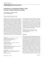
Figure 2. Nam Con Son sedimentary basin.

(a) Bouguer gravity anomaly, (b) Residual gravity, (c)Regional effect,(d) Inversed depth of basin,
(e) The gravity anomaly at the last iteration, (f) Rate of convergence

30

35

40


52

P.T. Luan, D.D. Thanh / VNU Journal of Science: Mathematics – Physics, Vol. 33, No. 2 (2017) 48-52

The hybrid technique is also applied in gravity field to determine the depth distribution of Nam
Con Son sedimentary basin. Study area is about 100,000 km2, ranging from 90N to 110N latitude and
106.50E to 109.50E longitude. The results are shown in Figure 2.
Figure 2a is the Bouguer gravity anomaly map presented by Bui Cong Que and Nguyen Hiep [9].
Figure 2b illustrates the residual gravity of Nam Con Son sedimentary basin obtained from the
Bouguer gravity anomalies by removing the regional effect (Figure 2c). Residual density of basin is
which was determined from density data of drillhole 21S - 1X [9].
Figure 2d shows the depth result of Nam Con Son sedimentary basin. Figure 2e shows gravity
anomaly at the last iteration. By compared Figure 2e and Figure 2b, it is clearly that the depth model
of Nam Con Son sedimentary basin obtained from the hybrid technique produces the gravity anomaly
very similar in shape to the residual gravity. The rate of convergence of method is fast, and it only
takes 5 seconds for calculation. The depths to the interface compare favorably with the results of
seismic exploration methods [9].
5. Conclusions
The computation results obtained from numerical and field examples showed that the hybrid
technique based on the FFT and space domain techniques would be a useful approach in gravity

interpretation, especially in inversion procedure. According to the technique, the gravity anomaly is
easily computed from Parker and Granser’s formula. Then, the depth to the interface is determined by
Bott’s approach. The obtained results compare very favorably with theoretical models and seismic
data. The computation speed of the hybrid technique is much faster than that of space domain
technique. Moreover, the depth results using hybrid technique are also more accurate than those using
Parker-Oldenburg method.
References
[1] R. L. Parker, The Rapid Calculation of Potential Anomalies, Geophys. J. R. astr. SOC. 31 (1972) 447–455.
[2] Oldenburg, The inversion and interpretation of gravity anomalies, Geophysics, 39 (1974) 526-536.
[3] David Gómez Ortiz, Bhrigu N.P. Agarwal, 3DINVER.M: A MATLAB program to invert the gravity anomaly
over a 3D horizontal density interface by Parker–Oldenburg’s algorithm, Computers & Geosciences, 31 (2005)
513–520.
[4] Young Hong Shin, Kwang Sun Choi, HouzeXu, Three-dimensional forward and inverse models for gravity fields
based on the Fast Fourier Transform, Computers & Geosciences, 32 (2006) 727–738.
[5] R. Nagendra, P.V.S. Prasad, V.L.S. Bhimasankaram, Forward and inverse computer modeling of gravity field
resulting from a density interface using Parker-Oldenberg method, Computers & Geosciences, 22 (1996) 227231.
[6] R. Nagendra, P.V.S. Prasad, V.L.S. Bhimasankaram, FORTRAN program based on Granser's algorithm for
inverting a gravity field resulting from a density interface, Computers & Geosciences, 2 (1996) 219-225.
[7] Bott, M.H.P, The use of rapid digital computing methods for direct gravity interpretation of sedimentary basins,
Geophysical Journal of the Royal Astronomical Society, 3(1960)63-67.
[8] Harald Granser, Three - dimensional interpretation of gravity data from sedimentary basins using an exponential
density – depth function, Geophysical Prospecting, 35(1987)1030 – 1041.
[9] Bui Cong Que and Nguyen Hiep, Geophysical field characteristics of Vietnam continental shelf and its neighbor,
Project final report No. 48-B.03.02, 48-B marine research program, Hanoi, 1990. (in Vietnamese)