DSpace at VNU: A new method for separation of randow noise from capacitance signal in dlts measurement
Bạn đang xem bản rút gọn của tài liệu. Xem và tải ngay bản đầy đủ của tài liệu tại đây (2.63 MB, 8 trang )
VNU JOURNAL OF SCIENCE. Mathematics - Physics T XVIII. N0 2 - 2002
A N E W M E T H O D F O R S E P A R A T IO N O F R A N D O M N O IS E
F R O M C A P A C I T A N C E S IG N A L IN D L T S M E A S U R E M E N T
Hoang Nam Nhat, Pham Quoc Trieu
D epartm ent o f P h y sics y College o f S cien ce - V N U
A bstract. We introduce a new statistical method f o r separation o f random noise
fro m capacitance signal in D L T S m easurement.
F o r the in te rfe re n ce o f a white
random no ise £ with capacitance signals (7(0 of general expo nen tial fo rm
%
we show that, noise £ and e m issio n fa c t o r 6 are statistically different and can be well
separated each fro m other.
Theoretical fo rm a lis m f o r re co n stru ctio n o j noise-free
capacitance signals based on d ete rm in a tio n o f e m is s io n fa c to r is presented. The
method has been tested f o r v a n o u s sign a l-to -n oise ratio s fro m 1000 down to 10 .
S im u la tio n and examples are given.
Abbreviations
T tem perature
t tim e
C n (t) normalized capacitance at certain fixed T
L ( t ) L n ( C n ) e.g. natural logarithm of normalized capacitance at fixed T
p(£) density probability of random variable £
P (0 cumulative probability of random variable £
6 , emission factor of a deep center I
i?, activation energy of a deep center i
LJi ratio E i / k between E i and Boltzmann constant k for a deep center i
Definition of terms
1 . We will work with a so-called n o rm a lized capacitance C n at certain temperature
T defined as C n { t ) = Cq 1 X [C(/) — Cl), where C{) is C ( t ) at t = 0 and C \ is C ( t ) at
t. = oo. For 0 < t < 0 0 , C n (t) always specifies relation 0 < c n (t) < 1 , this means that
L n ( Cri) has definite and negative value within this range. Taking Ln on Ln { Cn) is not
possible bu t L n \ - L n ( C Ti)} has definite values.
2. The average value of a variable X defined on the probability distribution p(£) of
a random variable £ will be denoted by < X
. Practically we will consider :.he average
values of X = Exp { - E / k T ) and L n ( X ) according to probability distribution of emission
factor p (e ). Generally, the small p — s denotes density function where the capital p - s
means cum ulative probability.
3. A random noise with uniform probability distribution in whole range of frequen
cies is called white ran d om noise. White random noise in restricted area of frequencies
will be called white gaussian n oise if possessing Gaussian distribution.
32
A
n e w m e th o d fo r se p a ra tio n o f r a n d o m
n o ise fr o m .
33
I. Introduction
Tilt 1 oenu rrnec of noise always disturbs the signals and lowers the* quality of mea
surement or rvrii
it iiujx>ssiK>lo. In a fine-tuned measurement system like DLTS the
or.nuTPWP of noisr is rxtmnolv critical for many important cases. Doolittle Kf, Rohatgi
lirivi* trslrd thí' iuiK t ionnlit V of various techniques when noise iii1 .ori’(T<\s and there have
observed tlicit nil hrliuiqiK's Ini loci (‘Xcopt for lock-in [ 1 j. In general tli
either temperature or frequency micro-fluctuation and ii) white random noise which pro
duces constant mhlitivr out puts to the signal at all temperatures and frequencies. While
the first kind of noise always disturbs signal exponentially, i.e. the measure of disturbance
grows exponentially wit Ik inrrrasrd time or temperature variable, th<* white random noise
is statistically indcprihicnt to I hr Signal. In this paper we will focus on this kind of noise.
T1kt<* an* many hrlmiqws how to filter the random noise, probably the most popular
oiu‘ is lock-in. In gcAin*nil tliOM1 t«‘cliniques may he considered a»s the correlation averaging
techniques which H'lv 0 1 : tlir correlation between input and output and/or the averaging
of signal ov«*r prrsH timo period I2|. They major disadvantage is that the smooth local
St nu t lire of signal within the preset time is usually removed together with t he averaging
process so 1 1 0 information is thru available for examination of close-spaced states. Obvi
ously. the prak struct tin' of any correlation integral of signal is more widened and more
smooth('ii(‘(l thiui of llìí' siftmil itself. Thus when the close-spaced (loop levels occur (and
îhrir DLTS linger prints overlap) the correlation averaging techniques usually U'acl to the
average value, not to the real ones. In this paper we discuss a new method for recovering
signal from lioisr while* preserving the signal original structure. The method is based on
tho differences in statist k ill brhaviors of signal and noise and is able to separate thorn ill
hravy noisy environment dur tu their characteristic signatures. The mathematical concept
is discussed in section II and ill section I II we introduce the full automated computer-based
prom.lurr for rmmstrucnng emission factor and thus the capacitance signal. The applica
bility of this promlun* ir* illustrated by simulation for sample with two preset close-spaced
deep levels and tlion tested in measurement with SiAu sample.
II. Statistical theory of interference of random white noise and exponential
signal
a ) S t a t i s t i c s o f e m i s s i o n f a c t o r 'p(e) i n a b s e n c e o f n o i s e
At each time / and fixed temperature T, the average value of emission factor € is
given by: < ( > ỵ2 ,p i(t)< :i where p-i(e) is a statistical weight for emission factor i. To
(Irtermim* the density probability function p(f.) wo perform the calculation for all measured
t:
{ L n \ C n(t)
} t — €f —< € > .
W ith respect to this distribution C n reads:
c
„
Exp!-
<
(
>
t
\
~
Expj- / ^
p,(c)et ] = n , E x p [ - i p , ( f ) f , ] .
( a *l)
H oang N a m Nhaty P ham Quoc Tri.eu
34
Denote c , = Exp[-£p,(f.)€i] we have the emission law for the close-spaced deep centers:
Cn = TUCi
(a.2 )
C i may be refereed to as t he p a rtia l capacitance of deep center i in statistical distribution
p(e)b) S t a t i s t i c s o f a c t i v a t i o n e n e r g y p ( E ) i n a b s e n c e o f n o i s e
Define x t = Exp( —E i / k T ) with E i is activation energy of deep center i. We have
Ln(A'i) = —E i / k T . Giving any probability distribution p {ri), the averages < L n ( X ) > n
and - < E > r? / k T must be identical. To determine the density probability function p(r/)
we perform the calculation for all measured t (with respect to that e = p T 2 E x p ( - E / k T )
where p is a constant):
{ v = L n { - r l T - * L n C n ( t ) } } t = { L n ( p ) - E / k T } t.
As seen, p(rj) does not reveal < E > v directly but < L n ( p ) - E / k T > v
holds fixed we may suppose that:
< L n ( p ) - E / k T > f;= L n (p )- < E / k T
As consequence p (£ ) = p(rç).
( b. l )
in ease L n ( p )
L n (p )- < £ > „ /fcT.
(b.2)
However, statistics (b.l) always produces < L n ( p ) -
E / k T > ff not < E > n in general.
c ) R e l a t i o n be tween p (f ) a n d p { E )
Suppose that (b.2) holds e.g. p ( E ) = p(f?). Ill term of < E >,), the average
< L n X >TJ reads:
< L n X > „ = - < E > n / k T = ~ ^ Vl{ E ) E J k T .
i
(c.l)
Emission factor becomes < e > , = p T 2Exp(< L n X
Whi le in term of < X >€,<
e >=
— p T 2 Y ì i P Ì { e) X i — p T 2 < X > e . Comparing these two relations leads
to:
L n < X > E = < L n X >r> .
(c.2)
We use this relation to check how much p(e) and p ( E ) differ each from other. If they
differ too much then the relation (b.2 ) may not hold for the case under investigation. The
physical meaning of (b.2 ) is that the noise effecting activation energy does not influence
level concentration and capture cross-section, th at is to say, E and L n ( p ) are statistically
independent.
d ) S t a t i s t i c s o f e m i s s i o n f a c t o r p(e) i n o c c u r r e n c e o f w h it e r a n d o m
n o is e
With existence of a random white noise, capacitance signal has the form:
C n = Noise-1-Exp[— < e > t\.
(d.1 )
A
new
m e th o d f o r s e p a m tio n o f r a n d o m
35
n o ise fr o m .
Rr-write C n to:
Cn
ICxpf— < ( > /]( 1 + Noise/Exp[- < € > t\)
and put:
Noise1
K.Exp[- < 6 > /ỊExpị—£/],
(ii.2)
when' K is constant aiK. £ is i\ random variable. Wo havo f'n a's:
c u - Exp[— < f > t](l + /cExp(-£fị).
D r n o tr o , = Exp- — < f > 1 .
c\
r„ = C Q
( 1 -r/\E x p - £ / ; ) and
— (C{ - 1 )/k :
o rC + n = c < (1 + k Q „ ) .
((1.3)
This moans that the cnpacit.rUKT transicMit in
occurrriier of noisr follows relation (a.2 ) for
closo-spacrd deep centfTs. r.u,. random noise
behaves as if it is a drop miter. This would
not he true if £ does not have; (Irnsity prob
ability similar to On . Fortunately, for ar
bitrary positive noise lcvrl Noise] (‘quation
(d.2) always has solution £ Lĩ ỉ ( Noise/*;)' 1/f
— < ( >. If [Noise is a random noiso with
uniform density, than £ has density proba
Í [a.u]
bility of L//(Noìs('/k) ]/t -~ < < > which is
practically the same as C n . (Sor Fig.l)
Fig. 1. Density probability p(£) of £=Ln
Clearly, for all measured / th(‘ statistics p { f ) :
(Noise/K)'1/l- <£>
{ Ỉ M C r > r l / t }t = { - < f > + f£}r,
(d.4)
where = { L n ( \ -f tfKxpi—£/j) 1 f} will re
veal average value of { — < ( > -fir} which
differs generally from (a. I). Fig.2 shows p(e)
for 3 different T . As seen, while at the middle
T the real f peak is high and proportional to
the noise peak
, at the high T the real e
peak is much smaller than tho noise peak
The side-effect of is that it widdens
the width of a delta-like (a. I) peak with the
amount proportional to <
>. One mav
expect that if < e > and are absolutely ad
ditive than the distribution spectrum of (cl.4)
Fig,2. Spectrum |Ln(Cn)'ỉ/f)ị at
will contain only one smooth Gaussian peak.
various temperature T. Noise=2%
However Fig.3 shows two different areas, one
of Cn unit.
corresponds to < e > and the other to €£.
This separation is true with two exceptions, the first occurs at low T when C n ispractically
equal
1and the second occurs at high T when Cn is near 0. In both cases, noise
so dominating that spectrum { L n ( C n ) ~ i ^t}t contains only values of
becom es
Hoang N a m N h a t , P h a m Quoc Tineu
36
e) T e m p e r a t u r e d e p e n d e n c e o f s i g n a l n o i s e s e p a r a t i o n i n { L n { C n) ~ ì ỉ t }t. s p e c
trum
There exists a threshold temperature
Tcrit where < e > is small enough and can not
be distinguished from €£. Let ớ ị and ơ ị be
variance of < 6 > and <
>, the criteria for
threshold temperature T crtt is that at Tcrit
the displacement < € > — < € $ > becomes
proportional to (ơf — ớ ị ) / 2 . This relation
is used to filter-off the noise where no signal
structure is seen:.
Fig. 3. The exitstence of two different
area for <£> and e* at noise level 5%,
10% and 2 0 % of Cn unit
(< e > - < * > ) Trrtt
fe.l)
III. Simulation and measurement
a ) P r o c e d u r e f o r the r e c o n s t r u c t i o n o f n o i s e - f r e e c a p a c i t a n c e s i g n a l
Data in the capacitance transient measurement are usually c o l l e c t e d at preset tem
perature T when the emission factor e can be considered as constant. To obtain the
statistical characteristics of e we should measure C n { t ) as dense as possible. However
the number of several hundreds data is adequate and 1 0 0 0 recorded data provide quite
satisfied results on simulation.
At the first step a logic circuit should be
available' to transform C n (t) into Ln[Crn(/-)'~1^]
and then into L n \ —t ~ l T ~ 2L n C n {t)}- This is
easy w ith com puter. The sta tistics p(c) is ob
tained after recording all L n [ C n ( t ) ~ l / i ] and sim
ilarly p(rj) by all L n [ —t ~ l T ~ 2L n C n (t)}. Two
statistics are then checked against each other
using relation (c.2) to see if p { E ) can be set
equal to p ( 7 7 ). If p ( E ) = /;(?/) holds we hâve
a simple case of one noise-free center, other
wise overlapped centers occur and noise should
be filtered. A numeric calculation of deriva
tion [dp(e)/de] should provide peak value fmax
of p(e). As noted before, we have two differ
ent cases: i) at the extremely low and high end
T there is only one e.£ peak. This noise-driven
exponentially-distributed peak should be removed
Fig. 4. (a) Un-filtered signal Cn(t);
(b) Cn(t)c reconstructed by Enwu;
(c) Cn(t)i obtained using lock-in;
(d) Cn(t)ç reconstructed bv
Noise = 2% of c„ unit
A
n e w m e th o d fo r se p a ra tio n o f r a n d o m
n o ise fr o m .
37
since it does not rorn spuinl to signals and contains no information about omission factor;
ii) i\i the middlo nuụ>,<' T (here arc two peak values, one corresponds to emission factor
f and thí' second relrrs to fi. They can be distinguished easily since p (e ) is a delta-like
Gaussian symmetrical (listribution while* p(c^) is a wide-spread asymmetrical exponential
OIK'. Some statistical trsis exist to help to automate the selection process.
Normally whoii measurement is kept ill
a roasouahlo T rangi1. the first case should not
occur and wo should only obsc-TVi1 the change
in prak bright for 'max
f Ẹ wli(‘n T varies.
Wit.h T increased poak f„,ax also grows and
bright ratio f./f£ iTiichi's maximum a! certain
T . Tho height rat io ( / ( c is proportional to
signal-to-Iioise ratio at preset T. If T grows
further, noise-đriVH» ft becomes higher and
may grow faster than ' m;ix- At extreme T
noise may even dominate over signal. This is
duo to thí» fact that i\i extreme high T the
C n (t) is practically ZCTOCM'I and we measure
T[K]
only noise. On simulation we have observed
that tlu* signal is still separable from noise
Fig. 5. DLTS finger-prints obtained from
at noise level 1 0 -times higher than the sig
(d) c n(t)eand (b) Cn(t)4. The first
nal. By averaging U'cln.ique oii(‘ would ob
discovers the real center and the second
tain false average at (ftniiX4- < fc > ) / 2 inshows the false ones. Noise=2% of Cn
Stead of real value4 f max Once 6 max is €<)1unit
lectod for each T . th<‘ noisf'-free capacitance
curve C n (t) can be reconstructed. Fig.4 com
pares c „ (/.)*• reconstructed by €max and the
capacitance signal obt ained by lock-in. Fig.5
shows DLTS finger-prints obtained using C n { t ) {
and C n ( t ) ^ Clearly, noise participates as a
set of emission cent (MS.
b)
S i m u l a t i o n f o r s a m p l e w it h tw o
c l o s e - s p a c e d d e e p le v e ls
The above* procedure has been tested
on simulation for a sample with two preset
close-spaced dee]) levels at 0.30 oV and 0.38
oV. Capture-cross sortions have been sot. at
1.0 X 10 ƯJcrn 2 and 2.0 X 10- 1 5 cm2, respec
tively. Both level concent rat ions wore 0.1 X
10” 1 5 cm~ 3. Constant random noise at 2%,
3% and 5% of signal maximum was added to
output.. Then the out-put. was filtmul-off a)
using lock-in and h) using p( f ) statistics.
T[K]
Fig. 6. DLT5 s p e c t r a obtained using (a)
lock-in filtered signal and (b) p(e) filtered
signal
Hoang N a m N h a t , P ham Quoc Trieu
38
Level analysis was carried out using the classical Lang’s DLTS scheme [3| for two cases:
a) filtered by lock-in; b) filtered by p (f ). Fig . 6 shows the resulting DLTS spectra for these.'
cases at noise 2%. As seen p(c)-filtered signal reveals the two preset close-spaced levels
while the lock-in filtered signal sees only their average at 0.34 eV. As noise increases the
spectrum of nil-filtered signal becomes unstable and failed to provide meaningful result .
c)
M e a s u r e m e n t w it h S i A u s a m p l e
The measurement was carried oil SiAu
sam ple.
T his sam ple has been investigated
by Fourier DLTS [4] on BIO -RAD’s DLTS
equipm ent at Center for M aterials Science,
Faculty of Physics, Hanoi University of Sci
ence and 3 different levels were shown. The
re-examination of the widdening of }){(■) peak
has reveal the interference of a constant white
random noise at 1.2% of maximal signal. Af
ter filtering off noise the reconstructed noisefree data was used for Fourier calculation and
the resulting 1)1 coefficient, is plotted in Fig.7.
As seen there are at least 2 more levels. All
of them are close-spaced to the existing ones
and did not appear in the original Fourier
calculation using un-filtered signal.
Fig. 7. Temperature dependence of
fourier coeficient bl for (a) unfiltered
signal and (b) p(e) filtered signal
IV. Conclusion
The method is officient to recover signals from noise in heavy noisy environment
when signal-to-noise ratio drops below 1 0 . Unlike averaging techniques, which take av
erages of signals and noise over certain time period and usually remove the local smooth
structure of signals within this period, the present method is able to separate signals di
rectly from noise due to the difference in their statistical behaviours. The method can
reveal the real values of signals while reserving the signal original smooth struc ture, which
is significantly important for obtaining the information about the existence of close-spaced
deep levels. Some modem method like Laplace DLTS [5, 6 ] is extremely sensible for noise
so the reconstructed noise-free data would be helpful to reduce instability of such met hods.
References
1 . W.A. Doolittle
A. Rohatgi, ./. A p p L Phys. 75(1994).
2 . M. Schwartz et al., C oram . System s & Techniques, McGraw-Hill, 1966.
3. D .v . Lang, J. Appl. Phys. 45(1974).
4. S. Weiss & R. Kassing, S o lid State E le c tro n ic s , Vol. 31, 12(1988).
5. s.w . Provencher, Com p. Phys. Com m un.y 27(1982) p.213
6 . L. Dobaczewski k. A.R. Peaker, 1997, />
A
new
m eth o d fo r
s e p a ra tio n
o f ran d o m
n o is e
fro m .
39
TAP CHÍ KHOA HỌC ĐHQGHN, Toán - Lý. T XVIII. So 2 - 2002
MỘT PHUƠNG PHÁP MỚI TÁCH N H lỄ ư
TỪ TÍN HIỆU PHỔ QUÁ ĐỘ TÂM SÂU
H o à n g N a m N h ậ t, P h ạ m Q u ố c T r iệ u
Khoa Lý, Đại học Khoa học T ự nhiên - ĐHQG Hà Nội
Bài báo nàv giới thiệu một phương pháp thống kẻ để tách nhiẻu ngẫu nhiên từ tín
hiệu diện dune trong phép đo phổ quá độ các tâm sâu (DLTS). Để tách biệt nhiẻu ngẫu
nhiên £ với tín hiệu điện dung c.(t) dạng hàm mũ Coe“ €í, các tác giả đã chỉ ra nhiẻu í và
hệ số phát xạ e là có thể tách biệt. Phương pháp này đã được thử cHo các tỷ số tín hiệu
trên tạp khác nhau từ 1000 đến 10. Sự mô phỏng và các ví dụ đã được chi ra.