DSpace at VNU: Electronic and magnetic properties of C-60-Fe-n-graphene intercalating nanostructures (n=1-6) predicted from first-principles calculations
Bạn đang xem bản rút gọn của tài liệu. Xem và tải ngay bản đầy đủ của tài liệu tại đây (1.74 MB, 5 trang )
Chemical Physics Letters 618 (2015) 127–131
Contents lists available at ScienceDirect
Chemical Physics Letters
journal homepage: www.elsevier.com/locate/cplett
Electronic and magnetic properties of C60 –Fen –graphene intercalating
nanostructures (n = 1–6) predicted from first-principles calculations
Hung M. Le a,b,∗ , Wilson K.H. Ng a , Hajime Hirao a,∗
a
Division of Chemistry and Biological Chemistry, School of Physical and Mathematical Sciences, Nanyang Technological University, 21 Nanyang Link,
Singapore 637371, Singapore
b
Faculty of Materials Science, University of Science, Vietnam National University, Ho Chi Minh City, Vietnam
a r t i c l e
i n f o
Article history:
Received 10 September 2014
In final form 21 October 2014
Available online 30 October 2014
a b s t r a c t
Graphene and C60 can establish coordination bonds with transition metal atoms/clusters. Using firstprinciples modeling methods, we explore the C60 –Fen –graphene intercalating nanostructures (n = 1–6),
which may have potential applications in, e.g., spintronics. Twelve optimized configurations are found to
possess good energetic stability (with binding energies of 4.22–20.54 eV). Eleven structures have different
magnitudes of magnetism (2.00–12.75 B /cell), whereas one is non-magnetic. The magnetism is highly
correlated with the bonding orientations between Fe atoms and C60 . Seven nanostructures possess good
half metallicity (with the spin polarization effects >0.8), while the non-magnetic structure is found to be
insulating.
© 2014 Elsevier B.V. All rights reserved.
1. Introduction
Since the successful experimental synthesis of graphene, a
material that features a two-dimensional carbon-made structure, many advanced technologies have been invented through
its utilization. At the nanometer scale, graphene has remarkable
mechanical stability because of the fully sp2 -bonding arrangement of carbon atoms [1]. Moreover, graphene is regarded as
a zero-gap semiconductor that exhibits superconductivity and
potentially offers useful applications in electronic devices [2]. Reaction catalysis is another noticeable application because graphene
can be employed as a hosting material to carry catalyzing metal
atoms/clusters/complexes [3–5]. For that reason, the chemistry of
metal-bonding interactions of graphene is an important aspect that
has been intensively investigated over the past few years [6–8].
The metal–graphene contact is formed upon hybridization of d and
p orbitals, similar to that in the intercalating structures of metal
and benzene [9]. The sp2 bonds are responsible for the formation
of a graphene monolayer; however, the 2pz orbitals, which are not
involved in the sp2 bonds, tend to interact with the vacant d shells
of metal atoms and form coordination bonds. So far, there have
been a large number of experimental studies of metal–graphene
nanostructures, such as those involving Ni [10], Au, Fe, Cr [11–13],
∗ Corresponding authors.
E-mail addresses: (H.M. Le),
(H. Hirao).
/>0009-2614/© 2014 Elsevier B.V. All rights reserved.
or Ag [14]. By employing electrolysis, Zhang et al. [15] investigated
the intercalating compounds of iron chloride on graphite. In addition, there have been efforts to attach graphene on metal surfaces
to derive interesting electronic properties [16].
Theoretical and computational investigations of graphene–
metal interactions have been conducted using density functional
theory (DFT) calculations [17,18]. Significant achievements in
graphene research have been attained during the past few years,
which have enhanced attention to the electronic and magnetic
properties of graphene. Importantly, Nakata and Ishii have provided theoretical evidence that 3d transition metals bind strongly
to graphene [19]. Moreover, the attachment of various types of
ligands on graphene via a transition-metal atom bridge has been
investigated in several previous studies [6,9,20,21]. Recently, we
have explored C60 –M–G nanostructures, in which buckminsterfullerene [22,23] (C60 ) was steadied on a graphene surface via one
bridging transition-metal atom [4,24]. Interestingly, when Cr, Mn,
Fe, or Ni is used as a bridging metal atom, C60 –M does not stand
upright on graphene; instead, we observe geometry distortions
that correlate with spin polarization in the 3d orbitals and dispersion interactions between graphene and C60 . We hypothesize
that such a geometry distorting feature may be effectively exploited
to design new nanostructures, in which multiple transition-metal
atoms are arranged in a crown-like manner. This strategy may allow
one to construct more stable graphene–metal–C60 nanostructures
that might find applications in spintronics or catalysis [25]. In this
Letter, we present a DFT investigation of bridging C60 and graphene
using several Fe atoms (up to six atoms).
128
H.M. Le et al. / Chemical Physics Letters 618 (2015) 127–131
Table 1
Binding energies, average Fe stabilization energies, MT and MA for the investigated
nanostructures.
Fe distribution
C60 –Fe–G
Figure 1. C60 steadied on graphene using six bridging Fe atoms. Twelve configurations (pre-optimized) based on Fe allocations are suggested: (a) C60 –Fe–G, (b)
C60 –Fe5 –G, (c) C60 –Fe6 –G, three C60 –Fe2 –G configurations, namely (d) (1,2), (e)
(1,3), and (f) (1,4), three C60 –Fe3 –G configurations, namely (g) (1,2,3), (h) (1,2,4),
and (i) (1,3,5), and three C60 –Fe4 –G configurations, namely (j) (1,2,3,4), (k) (1,2,3,5),
and (l) (1,2,4,5). For convenience, the given nomenclatures are used to address the
structures throughout the Letter.
2. Computational details
DFT calculations are executed using the Quantum
Espresso (QE) package [26]. Specifically, we employ the
Perdew–Burke–Ernzerhof (PBE) exchange-correlation functional [27,28] with the ultrasoft pseudopotentials [29,30] (USPP).
The kinetic energy cutoff for plane-wave expansion is set to 45
Rydberg. The empirical corrections for long-range dispersions are
also included [31,32]. To approximate the continuity of energy
bands, we employ the Gaussian smearing technique with a
small smearing width (0.002 Rydberg). Structural optimizations
are performed with an energy-convergence criterion of 10−6
Rydberg/cell. Initially, full structural optimizations are executed
at the -point by relaxing the atomic positions and unit cells
simultaneously. Then, the final relaxed structures are determined
by further relaxing the atomic positions with a k-point mesh of
(6 × 6 × 1).
The theoretical models have two-dimensional characteristics
and consist of three major building units: a periodic graphene
monolayer (54 C atoms), bridging atoms (i.e. Fen ), and C60 . In
those two-dimensional slabs, the length of c-axis is set to 40 Bohr
˚ to allow vacuum treatments in the z direction perpen(21.17 A)
dicular to the graphene sheet. In the C60 –Fe–G structure (Figure
S2, Supplementary Material (SM)), C60 –Fe does not stand upright
on the graphene sheet, and Fe interacts with only two C atoms in
C60 . In Figure 1, we show a complex structure with a maximum
load of six Fe atoms, which fully interact with a honeycomb ring
of C60 . Also, all other possible structures of C60 –Fen –G (n < 6) are
constructed. For illustration purposes, the top and side views of all
optimized C60 –Fen –G structures are presented in the SM.
After a geometry optimization, the binding energy of a complex
nanostructure with n Fe atoms can be calculated using the following
equation:
Ebinding = EC60 + nEFe + EG − Estructure ,
Ebinding
(eV)
ES
(eV)
MT
(B /cell)
MA
(B /cell)
4.22
4.22
2.00
3.09
7.62
6.78
6.83
3.81
3.39
3.42
4.11
0.00
4.05
6.33
0.00
5.40
C60 –Fe2 –G
(1,2)
(1,3)
(1,4)
C60 –Fe3 –G
(1,2,3)
(1,2,4)
(1,3,5)
10.68
10.38
9.74
3.56
3.46
3.25
6.13
6.11
6.00
8.58
8.51
8.02
C60 –Fe4 –G
(1,2,3,4)
(1,2,3,5)
(1,2,4,5)
13.88
13.98
14.05
3.47
3.49
3.51
8.50
8.14
8.09
11.31
10.55
11.30
C60 –Fe5 –G
17.73
3.55
10.36
14.12
C60 –Fe6 –G
20.54
3.42
12.75
16.60
3. Results and discussion
As shown in Table 1, with a full load of six Fe atoms, the
C60 –Fe6 –G nanostructure (Figure S3, SM) is highly stable with a
binding energy of 20.54 eV. On average, the stabilization energy
arising from each Fe atom in this case is 3.42 eV, which indicates
good stabilization of the nanostructure, although this stabilization
energy is lower than that of C60 –Fe–G (4.22 eV). The DOS data allow
us to estimate the total magnetization (MT ) and absolute magnetization (MA ) as reported in Table 1.
MT and MA of C60 –Fe6 –G are calculated as 12.75 and
16.60 B /cell, respectively. Such ferromagnetism is mainly produced by the strong spin polarization of the Fe atoms in the
nanostructure (with the major contribution of d orbital polarization). Recall that in a previous work [24], with the use of one Fe
atom, C60 –Fe–G was reported to exhibit a total magnetic moment
of 2.00 B /cell (Figure 2a), which is slightly smaller than one sixth
(1)
where EC60 , EFe , and EG are the total energies of C60 , an isolated Fe
atom, and the periodic graphene layer, respectively, while Estructure
denotes the total energy of the complex obtained from DFT calculations. For fair comparisons among the investigated cases, we define
average stabilization energy for a C60 –Fen –G nanostructure as
ES =
Ebinding
n
(2)
Figure 2. Spin-polarized total DOS (left panels) and PDOS of Fe atoms (right panels) in (a) C60 –Fe–G, (b) C60 –Fe4 –G (1,2,3,4), (c) C60 –Fe4 –G (1,2,3,5), (d) C60 –Fe4 –G
(1,2,4,5), (e) C60 –Fe5 –G, and (f) C60 –Fe6 –G. The Fermi level is positioned at 0.
H.M. Le et al. / Chemical Physics Letters 618 (2015) 127–131
Table 2
Magnetic contributions (B ) from Fe atoms (and their 3d shells) and spin polarization effects for the investigated C60 –Fen –G nanostructures.
Fe distribution
Fe magnetic contribution
(B )
Total
C60 –Fe–G
P
3d
2.33
2.22
1.00
C60 –Fe2 –G
(1,2)
(1,3)
(1,4)
4.81
0.00
3.68
4.75
0.00
3.57
1.00
–
0.87
C60 –Fe3 –G
(1,2,3)
(1,2,4)
(1,3,5)
7.01
6.80
6.42
6.87
6.63
6.19
0.81
1.00
1.00
C60 –Fe4 –G
(1,2,3,4)
(1,2,3,5)
(1,2,4,5)
9.46
8.27
9.32
9.30
8.10
9.16
0.61
0.76
0.68
11.91
14.27
11.75
14.14
0.39
0.89
C60 –Fe5 –G
C60 –Fe6 –G
of MT exhibited by C60 –Fe6 –G. Interestingly, we observe an alternate pattern of Fe occupations in C60 –Fe6 –G: three are closer to
C60 and possess slightly larger magnetic terms (2.50 B ), whereas
the other three are closer to graphene and possess smaller terms
(2.25 B ) as illustrated in Figure 2f. Moreover, the Löwdin charge
[33] analysis indicates that Fe2 , Fe4 , and Fe6 have smaller positive
charges than the others (see Table S1, SM).
The half-metallicity is an interesting feature that can be
observed in several nanostructures. In those nanostructures, while
one electronic spin state (up) indicates insulation, the other spin
state (down) is conductive. In a typical case of perfect halfmetallicity, the spin-up DOS should completely vanish at the Fermi
level. Particularly in the C60 –Fe6 –G case, the spin-up DOS does not
vanish at the Fermi level, but it is very small compared to the
spin-down DOS as shown in the total DOS diagram (Figure 2f).
Therefore, we regard this structure as an imperfect half metal. The
half-metallic property can be evaluated by the spin-polarization
effect P [34,35]:
P=
↑ (E ) −
F
↑ (E ) +
F
↓ (E )
F
↓ (E )
F
,
(3)
where ↑ (EF ) and ↓ (EF ) represent the spin-up and spin-down DOS
at the Fermi level, respectively. If P is unity, the material can be
regarded as a perfect half metal. Indeed, the spin polarization effect
of C60 –Fe6 –G is 0.89. In the C60 –Fe–G case, the spin polarization
effect is determined to be unity, which indicates a good half-metal.
For convenience, we summarize the magnetic contributions from
the metal atoms (and their 3d orbitals) and the calculated spin
polarization effects of the investigated nanostructures in Table 2.
When five Fe atoms are used (C60 –Fe5 –G), the bonding interactions between the metal atoms and graphene change significantly.
From the top view (Figure S4, SM), it can be seen that those five
Fe atoms constitute a pentagon-like structure. Closer inspection
shows that there are three types of Fe–graphene interactions with
different degrees of spin polarization. Two Fe atoms (2.52 B /atom)
interact with graphene via three Fe–C bonds, two Fe atoms
(2.33 B /atom) interact with full honeycomb units of graphene (but
dislocated from the center of the honeycomb rings), and one Fe
(2.24 B /atom) is located above the center of a honeycomb ring.
The difference in Fe locations can also be observed from the PDOS
of Fe (Figure 2e). The binding energy of C60 –Fe5 –G is 17.73 eV, while
the stabilization energy for one Fe atom is 3.55 eV, slightly higher
than that in C60 –Fe6 –G. C60 –Fe5 –G possesses weak half metallicity
because of its low spin-polarization effect (0.39).
129
As shown in Figure 1, three different C60 –Fe4 –G nanostructures
are optimized. When four Fe atoms are located at the (1,2,3,5)
positions (Figure S5, SM), the structure has an intermediate binding
energy (13.98 eV) and exhibits an intermediate magnetic moment
(8.14 B /cell) among the three possibilities. In this structure, four Fe
atoms fully interact with four corresponding honeycomb units from
graphene. Each of the first three metal atoms (Fe1 , Fe2 , Fe3 ) interacts with C60 via two Fe–C linkages, while the remaining Fe atom
(Fe4 in Figure 2c) fully interacts with a five-membered pentagonal
ring from C60 . Indeed, this special Fe atom has the smallest spin
polarization term (1.01 B ) among the four and a negative charge
(−0.06), while the other three Fe atoms have positive charges and
exhibit greater magnetic moments of 2.31–2.64 B . The partial DOS
(PDOS) profiles for Fe1 and Fe3 are very similar, and the highest
polarization term originates from Fe2 . Overall, this nanostructure
has a spin polarization effect of 0.76.
When four Fe atoms reside at the (1,2,3,4) positions (Figure S6,
SM), the resulting structure has a binding energy of 13.88 eV (lowest of the three cases), while it has the strongest ferromagnetism
of the three (8.50 B /cell). In this case, the Fe atoms are observed
to behave in slightly different manners (see Figure 2b). Each Fe
atom has a positive charge and produces a strong ferromagnetic
moment (higher than 2 B /atom). In the DOS plot (Figure 2b), it
is observed that the (1,2,3,4) structure has a low spin polarization effect (0.61). Similar to the case of (1,2,3,4), there are two
different types of Fe allocations in the (1,2,4,5) structure (Figure
S7, SM), which has the largest binding energy (14.05 eV) of the
three C60 –Fe4 –G cases. All four atoms are found to shift slightly
away from the center of the honeycomb rings in graphene and
each Fe interacts with two C atoms from C60 , which results in a
strong ferromagnetic moment (2.25–2.41 B /atom). Consequently,
a strong magnetic moment of 8.09 B /cell is found (but the smallest of the three C60 –Fe4 –G cases). Like in the cases of (1,2,3,4) and
(1,2,3,5), the (1,2,4,5) structure does not really possess the halfmetal characteristics, because there is still electron density in the
spin-up state at the Fermi level (see the DOS plot in Figure 2d),
and the spin polarization effect for the (1,2,4,5) structure is as low
as 0.68. Additional validation calculations are executed using QE
with the USPP and the Vienna Ab Initio Package [36–38] (VASP 4.6)
with the projector-augmented-wave method for the inspection of
ferromagnetic/anti-ferromagnetic states in C60 –Fe4 –G (1,2,4,5) and
three other structures (Figure S1, SM). We conclude that neighboring Fe atoms favor the ferromagnetic spin alignment and do not
have opposing magnetic moments.
There are three possibilities to distribute two Fe atoms in
C60 –Fe2 –G. In those three cases, the two Fe atoms are observed
to shift slightly away from the centers of the honeycomb units
in graphene; however, the major distinctions come from various
interacting schemes between Fe and C60 . When two Fe atoms are
placed in the (1,2) arrangement (Figure S8, SM) (resulting in an
˚ each Fe atom interacts with C60 via two
Fe–Fe distance of 2.47 A),
Fe–C linkages, receives a positive charge, and exhibits a large ferromagnetic moment (2.41 B per each Fe atom). Overall, the (1,2)
structure exhibits a total magnetic moment of 4.11 B /cell. From
binding energy calculations, it is shown that the (1,2) structure is
the most stable of the three C60 –Fe2 –G structures examined and the
corresponding average stabilization energy is the largest (3.81 eV)
of all structures reported in this study (excluding the C60 –Fe–G
case). According to the DOS distribution (Figure 3a), the (1,2) structure can be regarded as a perfect half-metal with the P value of 1.00
(largest among three C60 –Fe2 –G cases).
The (1,3) and (1,4) structures (Figures S9 and S10 in the SM,
respectively) are less stable, with the binding energies being 6.78
and 6.83 eV, respectively. It is seen from the DOS plots (Figure 3b
and c) that the (1,3) nanostructure is a non-magnetic and insulating material, while (1,4) possesses half-metallicity with the
130
H.M. Le et al. / Chemical Physics Letters 618 (2015) 127–131
Figure 3. Spin-polarized total DOS (left panels) and PDOS of Fe atoms (right panels)
in (a) C60 –Fe2 –G (1,2), (b) C60 –Fe2 –G (1,3), (c) C60 –Fe2 –G (1,4), (d) C60 –Fe3 –G (1,2,3),
(e) C60 –Fe3 –G (1,2,4), and (f) C60 –Fe3 –G (1,3,5). The Fermi level is positioned at 0.
spin-polarization effect estimated as 0.87. In the (1,3) case, two
Fe atoms play similar roles in the bonding interaction with C60 ,
and each of them establishes bonding to C60 via three Fe–C linkages. Interestingly enough, such an unusual interacting scheme
causes the spin-up and spin-down DOS to cancel each other out
and consequently produces a non-magnetic structure (illustrated
in Figure 3b). The band gap of this insulating case is very narrow
(0.09 eV) according to our band energy examination. Both Fe atoms
in the (1,3) case have negative charges. On the other hand, two Fe
atoms in the (1,4) case behave differently from each other. While
Fe1 (as denoted in Figure 3) makes bonds to a five-membered ring
from C60 and exhibits a weak ferromagnetic term (1.30 B ) with
a negative charge (−0.04), Fe2 interacts with two C atoms and
exhibits a stronger ferromagnetic moment (2.38 B ) with a positive charge (0.13). Unlike the other magnetic structures where Fe
atoms contribute ferromagnetic terms and C atoms contribute antiferromagnetic terms, the (1,4) structure is the sole case where Fe,
C60 , and graphene jointly contribute ferromagnetism.
With the inclusion of three metal atoms, each Fe is found to
interact fully with the honeycomb rings in graphene while binding
to C60 via two Fe–C linkages. When three metal atoms are located at
the (1,2,3) positions (Figure S11, SM), Fe1 and Fe3 behave similarly
in their interactions with graphene and C60 as proved by the PDOS
of Fe1 and Fe3 (with a magnetic alignment of 2.23 B /atom). Fe2 , on
the other hand, exhibits a larger magnetic contribution (2.55 B )
than the others. The total ferromagnetic moment of the (1,2,3)
structure (6.13 B /cell) is actually observed to be the largest of all
C60 –Fe3 –G cases. In the next structure having the (1,2,4) arrangement for three Fe atoms (Figure S12, SM), the role of each metal
atom is different from that of the others, as seen in the PDOS distribution in Figure 3e. This structure exhibits a magnetic moment with
an intermediate magnitude among three cases (6.11 B /cell). In the
last case, three Fe atoms are equally distributed on the graphene
sheet (Figure S13, SM), so that they interact with C60 in an almost
similar manner (see Figure 3f). As a result, they establish the same
spin polarizations, which produce an approximate magnetic alignment of 2.14 B /Fe atom. The total magnetic moment given by this
structure is 6.00 B /cell. It can be seen that the computed total magnetizations of three C60 –Fe3 –G structures vary in a small range.
Figure 4. Charge density plots of the planes containing three Fe atoms in the (a) (1,2,3) and (b) (1,2,4) C60 –Fe3 –G nanostructures. The Fe atoms are represented by red
spheres. (For interpretation of the references to color in this figure legend, the reader is referred to the web version of this article.)
H.M. Le et al. / Chemical Physics Letters 618 (2015) 127–131
Notably, all the investigated C60 –Fe3 –G structures possess semimetallicity. Among the three C60 –Fe3 –G nanostructures, the (1,2,3)
structure has the lowest spin polarization effect (0.81). At the same
time, this structure also has the largest binding energy and magnetic moment (shown in Table 1). In contrast, (1,2,4) and (1,3,5)
have perfect spin polarization effects (1.00), while they are quite
less stable (with binding energies of 10.38 and 9.74 eV, respectively)
and exhibit smaller magnetic moments (6.11 and 6.00 B /cell).
The interactions between intercalated Fe atoms and graphene
have large binding energies and thus can be regarded as strong
coordination bonds. Interestingly, this bonding interaction alters
the electronic structure of graphene by doping electron density
to build up the highest occupied bands in the -spin. Not only
does this behavior result in magnetism, but it also causes halfmetallicity of most nanostructures, as can be seen in Figure S14
(SM) where we observe significant contributions of C60 –Fen groups
at the highest occupied bands. Semi-metallicity, which arises from
the incorporation of the d-bands across the Fermi energy level, has
also been found in other carbon materials intercalated with transition metal atoms [20,39]. In cyclopentadienyl–Fe–carbon nanotube
(Cp–Fe–CNT) [39], the magnetic moment of Fe is quenched to 0.00
or 0.97 B /cell, whereas in benzene–Fe–graphene [20] and the current system, the magnetic moment of Fe remains large. The smaller
magnetic moment in Cp–Fe–CNT is due to the strong interactions
and multiple chemical bonds between metal and CNT. Another
notable difference between previous studies and ours is the slant
orientation of C60 in the one-Fe case, while the Cp ring and benzene
remain flat and preserve the Á5 and Á6 hapticities, respectively. In
fact, Á2 hapticity in organometallic compounds containing a buckminsterfullerene ligand is common [40].
It is of particular interest to inspect the Fe–Fe interactions, which
may affect the stability of the nanostructures to some extent. In
order to verify the possible interactions between Fe atoms, we
choose to examine charge density distributions in two C60 –Fe3 –G
models: (1,2,3) and (1,2,4). In the (1,2,3) structure, there are two
possible Fe–Fe bonds (with 2.37 A˚ in length), while in the (1,2,4)
structure, we suspect that there is only one Fe–Fe interaction
˚ because one Fe is distant from the other two Fe atoms. In
(2.35 A)
the two-dimensional charge density plots of the Fe atoms (Figure 4),
we observe that there are actually two weak Fe–Fe interactions
in the (1,2,3) case, while there is only one Fe–Fe interaction in
(1,2,4). Such metal–metal interactions explain why the stabilization energy of (1,2,3) is the largest and the stabilization energy of
(1,3,5) is the smallest. The contribution of metal–metal interactions
in structural stabilizations is also significant in C60 –Fe2 –G, because
the (1,2) structure with a Fe–Fe distance of 2.47 A˚ has the largest
stabilization energy.
a five-membered ring of C60 ). From the charge distribution plots
(Figure 4), it is observed that there is a weak Fe–Fe interaction
˚ which contributes
when the distance is relatively short (∼2.3 A),
somewhat to the enhanced stabilization of Fe atoms in the structures. Importantly, seven half-metals with spin polarization effects
greater than 0.8 are found. With the interesting magnetism and stability, the C60 –Fen –G nanostructures may find useful applications
in spintronics, catalysis, etc.
Acknowledgments
The authors thank the High-Performance Computing Centre at
Nanyang Technological University and the Institute for Materials
Research at Tohoku University, Japan (under VNU B2014-18-03) for
computer resources. This work is supported by a Nanyang Assistant
Professorship and an AcRF Tier 1 grant (RG3/13).
Appendix A. Supplementary data
Supplementary data associated with this article can be found, in
the online version, at doi:10.1016/j.cplett.2014.10.051.
References
[1]
[2]
[3]
[4]
[5]
[6]
[7]
[8]
[9]
[10]
[11]
[12]
[13]
[14]
[15]
[16]
[17]
[18]
[19]
[20]
[21]
[22]
[23]
[24]
4. Conclusions
In summary, the C60 –Fen –G nanostructures (n ≤ 6) investigated in this study are highly stable. The nanostructures seem
to be stabilized significantly with the average stabilization energies amounting to >3 eV. Most structures exhibit ferromagnetism
(except the C60 –Fe2 –G (1,3) case where magnetism vanishes and
a narrow band gap of 0.09 eV is open). The magnetic alignment
of each Fe atom exhibits dependency on the bonding situation
between graphene and C60 . For instance, when the metal atom is
bound to C60 via two Fe–C linkages, the electron spin in 3d orbitals
is highly polarized to produce a magnetization above 2 B . Otherwise, the metal atom exhibits a weak magnetic moment (when
it interacts fully with a five-membered ring from C60 ) or even
becomes non-magnetic (when it interacts with three C atoms from
131
[25]
[26]
[27]
[28]
[29]
[30]
[31]
[32]
[33]
[34]
[35]
[36]
[37]
[38]
[39]
[40]
R. Prasher, Science 328 (2010) 185.
A.K. Geim, K.S. Novoselov, Nat. Mater. 6 (2007) 183.
Y.-H. Lu, M. Zhou, C. Zhang, Y.-P. Feng, J. Phys. Chem. C 113 (2009) 20156.
H.M. Le, H. Hirao, Y. Kawazoe, D. Nguyen-Manh, Phys. Chem. Chem. Phys. 15
(2013) 19395.
L. Shang, et al., Angew. Chem. Int. Ed. 53 (2014) 250.
V.Q. Bui, H.M. Le, Y. Kawazoe, D. Nguyen-Manh, J. Phys. Chem. C 117 (2013)
3605.
H.R. Byon, J. Suntivich, Y. Shao-Horn, Chem. Mater. 23 (2011) 3421.
H. Huang, H. Zhang, Z. Ma, Y. Liu, H. Ming, H. Li, Z. Kang, Nanoscale 4 (2012)
4964.
I.S. Youn, D.Y. Kim, N.J. Singh, S.W. Park, J. Youn, K.S. Kim, J. Chem. Theory
Comput. 8 (2012) 99.
M. Weser, et al., Appl. Phys. Lett. 96 (2010) 012504.
R. Muszynski, B. Seger, P.V. Kamat, J. Phys. Chem. C 112 (2008) 5263.
W. Hong, H. Bai, Y. Xu, Z. Yao, Z. Gu, G. Shi, J. Phys. Chem. C 114 (2010)
1822.
R. Zan, U. Bangert, Q. Ramasse, K.S. Novoselov, Nano Lett. 11 (2011) 1087.
Y. Hajati, et al., Nanotechnology 23 (2012) 505501.
H.Y. Zhang, W.C. Shen, Z.D. Wang, F. Zhang, Carbon 35 (1997) 285.
J. Wintterlin, M.L. Bocquet, Surf. Sci. 603 (2009) 1841.
P. Hohenberg, W. Kohn, Phys. Rev. 136 (1964) B864.
W. Kohn, L.J. Sham, Phys. Rev. 140 (1965) A1133.
K. Nakada, A. Ishii, Solid State Commun. 151 (2011) 13.
P. Plachinda, D.R. Evans, R. Solanki, J. Chem. Phys. 135 (2011) 044103.
S.M. Avdoshenko, I.N. Ioffe, G. Cuniberti, L. Dunsch, A.A. Popov, ACS Nano 5
(2011) 9939.
H.W. Kroto, Nature 329 (1987) 529.
H.W. Kroto, J.R. Heath, S.C. O’Brien, R.F. Curl, R.E. Smalley, Nature 318 (1985)
162.
H.M. Le, H. Hirao, Y. Kawazoe, D. Nguyen-Manh, J. Phys. Chem. C 118 (2014)
21057.
A. Ludwig, et al., in: H. Zabel, M. Farle (Eds.), Magnetic Nanostructures, 246,
Springer, Berlin, Heidelberg, 2013, p. 235.
P. Giannozzi, et al., J. Phys.: Condens. Matter 21 (2009) 395502.
J.P. Perdew, K. Burke, M. Ernzerhof, Phys. Rev. Lett. 77 (1996) 3865.
J.P. Perdew, K. Burke, M. Ernzerhof, Phys. Rev. Lett. 78 (1997) 1396.
A. Dal Corso, Phys. Rev. B 64 (2001) 235118.
D. Vanderbilt, Phys. Rev. B 41 (1990) 7892.
S. Grimme, J. Comput. Chem. 27 (2006) 1787.
V. Barone, M. Casarin, D. Forrer, M. Pavone, M. Sambi, A. Vittadini, J. Comput.
Chem. 30 (2009) 94.
D. Sanchez-Portal, E. Artacho, J.M. Soler, Solid State Commun. 95 (1995) 685.
R.J. Soulen, et al., Science 282 (1998) 85.
V.Q. Bui, T.-T. Pham, H.-V.S. Nguyen, H.M. Le, J. Phys. Chem. C 117 (2013) 23364.
G. Kresse, J. Hafner, Phys. Rev. B 47 (1993) 558.
G. Kresse, J. Furthmüller, Comput. Mater. Sci. 6 (1996) 15.
G. Kresse, J. Furthmüller, Phys. Rev. B 54 (1996) 11169.
Z. Zhang, C.H. Turner, J. Phys. Chem. C 117 (2013) 8758.
A.L. Balch, M.M. Olmstead, Chem. Rev. 98 (1998) 2123.