DSpace at VNU: Rayleigh waves in an incompressible elastic half-space overlaid with a water layer under the effect of gravity
Bạn đang xem bản rút gọn của tài liệu. Xem và tải ngay bản đầy đủ của tài liệu tại đây (455.74 KB, 10 trang )
Meccanica
DOI 10.1007/s11012-013-9723-x
Rayleigh waves in an incompressible elastic half-space
overlaid with a water layer under the effect of gravity
Pham Chi Vinh · Nguyen Thi Khanh Linh
Received: 13 May 2012 / Accepted: 28 February 2013
© Springer Science+Business Media Dordrecht 2013
Abstract This paper is concerned with the propagation of Rayleigh waves in an incompressible isotropic
elastic half-space overlaid with a layer of non-viscous
incompressible water under the effect of gravity. The
authors have derived the exact secular equation of the
wave which did not appear in the literature. Based on
it the existence of Rayleigh waves is considered. It is
shown that a Rayleigh wave can be possible or not,
and when a Rayleigh wave exists it is not necessary
unique. From the exact secular equation the authors
arrive immediately at the first-order approximate secular equation derived by Bromwich [Proc. Lond. Math.
Soc. 30:98–120, 1898]. When the layer is assumed to
be thin, a fourth-order approximate secular equation
is derived and of which the first-order approximate
secular equation obtained by Bromwich is a special
case. Some approximate formulas for the velocity of
Rayleigh waves are established. In particular, when the
layer being thin and the effect of gravity being small,
a second-order approximate formula for the velocity is
created which recovers the first-order approximate formula obtained by Bromwich [Proc. Lond. Math. Soc.
P.C. Vinh ( )
Faculty of Mathematics, Mechanics and Informatics,
Hanoi University of Science, 334, Nguyen Trai Str., Thanh
Xuan, Hanoi, Vietnam
e-mail:
N.T.K. Linh
Department of Engineering Mechanics, Water Resources
University of Vietnam, 175 Tay Son Str., Hanoi, Vietnam
30:98–120, 1898]. For the case of thin layer, a secondorder approximate formula for the velocity is provided
and an approximation, called global approximation,
for it is derived by using the best approximate secondorder polynomials of the third- and fourth-powers.
Keywords Rayleigh waves · An incompressible
elastic half-space · A layer of non-viscous water ·
Gravity · Secular equations · Formulas for the
velocity
1 Introduction
Elastic surface waves in isotropic elastic solids, discovered by Lord Rayleigh [1] more than 120 years
ago, have been studied extensively and exploited in a
wide range of applications in seismology, acoustics,
geophysics, telecommunications industry and materials science, for example. It would not be far-fetched
to say that Rayleigh’s study of surface waves upon
an elastic half-space has had fundamental and farreaching effects upon modern life and many things
that we take for granted today, stretching from mobile phones through to the study of earthquakes, as addressed by Adams et al. [2].
The problem on the propagation of Rayleigh waves
under the effect of gravity is a significant problem in
Seismology and Geophysics, and many investigations
on this topic have been carried out, see for examples
[3–21].
Meccanica
The propagation of Rayleigh waves in an incompressible isotropic elastic half-space underlying a nonviscous incompressible fluid layer under the effect of
gravity was studied also by Bromwich [3]. In his study
Bromwich assumed that the fluid layer is thin and
the effect of gravity is small. With these assumption
the author derived the first-order approximate dispersion equation of the wave by approximating directly
the boundary conditions. However, as illustrated below in Sect. 2.1, that approximate secular equation is
not valid for all possible values of the Rayleigh wave
velocity (lying between zero and the velocity of the
bulk transverse wave in the elastic substrate). Based
on the obtained first-order approximate secular equation, Bromwich derived a first-order approximate formula for the Rayleigh wave velocity. Bromwich did
not consider the general problem when the depth of
the layer and the effect of gravity being arbitrary. This
problem is significant in practical applications.
The main aim of this paper is to investigate the general problem and to improve on Bromwich’s results. In
particular: (i) We first derive the exact secular equation
of Rayleigh waves for the general problem. From this
we arrive immediately at the first-order approximate
secular equation derived by Bromwich [3] and indicate that it is not valid for all possible values of the
Rayleigh wave velocity. (ii) Based on the exact secular equation the study of the existence of Rayleigh
waves is carried out. It is shown that a Rayleigh wave
can be possible or not, and when a Rayleigh wave
exists it is not necessary unique. Note that from the
first-order approximate dispersion equation derived by
Bromwich it is implied that if a Rayleigh wave exists it must be unique. (iii) When the fluid layer being
thin we establish a fourth-order approximate secular
equation and of which the first-order approximate secular equation obtained by Bromwich is a special case.
(iv) For the case of thin layer and small effect of gravity, a second-order approximate formula for the velocity is created which recovers the first-order approximate formula obtained by Bromwich [3]. (v) When
only the layer being thin, a second-order approximate
formula for the velocity is provided and an approximation, called global approximation, of the velocity
is derived by using the best approximate second-order
polynomials of the third- and fourth-powers.
We note that, for the Rayleigh wave its speed is a
fundamental quantity which is of great interest to researchers in various fields of science. It is discussed
Fig. 1 Elastic half-space overlaid with a water layer
in almost every survey and monograph on the subject
of surface acoustic waves in solids. Further, it also
involves Green’s function for many elastodynamic
problems for a half-space, explicit formulas for the
Rayleigh wave speed are clearly of practical as well
as theoretical interest.
2 Secular equation
2.1 Exact secular equation
Consider an incompressible isotropic elastic halfspace x3 < 0 that is overlaid with a layer of incompressible non-viscous water occupying the domain
0 < x3 ≤ h (see Fig. 1). The elastic half-space and
the water layer is separated by the plane x3 = 0. Both
the elastic half-space and the water layer are assumed
to be under the gravity. We are concerned with a plane
strain such that:
uk = uk (x1 , x3 , t),
p = p(x1 , x3 , t),
k = 1, 3,
u2 ≡ 0
φ = φ(x1 , x3 , t)
(1)
where uk and p are respectively the displacement
components and the hydrostatic pressure corresponding to the elastic half-space, φ is the velocity-potential
of the water layer with ∂φ/∂s as the velocity in the
direction ds (see [3]), t is the time. According to
Bromwich [3], the equations governing the motion of
the elastic half-space and the water layer are:
p,1 + μ
2
u1 = ρ u¨ 1 ,
u1,1 + u3,3 = 0,
p,3 + μ
2φ
=0
2
u3 = ρ u¨ 3
(2)
Meccanica
where commas indicate differentiation with respect to
spatial variables xk , a superposed dot denotes differentiation with respect to t, 2 f = f,11 + f,33 , ρ and μ
are the mass density and the Lame constant of the elastic solid. Addition to Eqs. (2) are required the boundary condition at x3 = h [3]:
gφ,3 + φ¨ = 0 at x3 = h
(3)
the continuity conditions at x3 = 0 [3]:
φ,3 = u˙ 3
at x3 = 0
(4)
μ(u1,3 + u3,1 ) = 0 at x3 = 0
(5)
˙
p + 2μu3,3 + g ρ − ρ u3 − ρ φ = 0 at x3 = 0 (6)
and the decay condition at x3 = −∞:
uk = 0 (k = 1, 3),
p = 0,
at x3 = −∞
(7)
where ρ is the mass density of the water, g is the
acceleration due to the gravity. Now we consider the
propagation of a Rayleigh wave, travelling with the velocity c (> 0) and the wave number k (> 0) in the x1 direction, and decaying in the x3 -direction. According
to Bromwich [3], the solution of Eqs. (2) satisfying the
decay condition (7) is:
p
= Qekx3 exp(ikx1 + iωt)
μk22
p,1
u1 = − 2 + Aesx3 exp(ikx1 + iωt)
μk2
p,3
u3 = − 2 + Besx3 exp(ikx1 + iωt)
μk2
(8)
(9)
(10)
φ = C cosh(kx3 ) + D sinh(kx3 ) exp(ikx1 + iωt)
(11)
where ω = kc is the circular frequency, k2 = ω/c2 <
√
k, c2 = μ/ρ, s = k 2 − k22 (> 0), Q, A, B, C, D
are constants to be determined from the conditions (3),
(4) and the relation ikA + sB = 0. Using Eqs. (8)–
(10) into Eq. (5) and taking into account ikA + sB = 0
yield:
2Q + (x − 2)Bˆ = 0
(12)
where Bˆ = B/k, x = c2 /c22 called the squared dimensionless velocity of Rayleigh waves and 0 < x < 1 in
order to satisfy the decay condition (7). From Eqs. (6),
(8), (10) and (11) we have:
μk22 Q + 2μ sB − k 2 Q
+ g ρ − ρ (B − kQ) − iρ ωC = 0
(13)
It follows from Eqs. (4), (8), (10) and (11):
D = iω(Bˆ − Q)
(14)
On use of (11) in (3) and taking into account (14)
yield:
(x − ε tanh δ)C = iω(Bˆ − Q)(ε − x tanh δ)
(15)
where ε = g/(kc22 ) (> 0) and δ = kh (> 0).
Since 0 < tanh δ < 1, it follows from (15) that:
x = ε tanh δ, because otherwise either Bˆ = Q or ε −
x tanh δ = 0. If Bˆ = Q then Bˆ = Q = D = C = A = 0
by (12)–(14) and ikA + sB = 0. It is impossible because this leads to a trivial solution. If ε − x tanh δ = 0,
from x = ε tanh δ we have immediately tanh δ = 1.
From (15) and x = ε tanh δ we have:
C = iω(Bˆ − Q)f (x, ε, δ)
(16)
where:
ε − x tanh δ
x − ε tanh δ
With the help of (16), Eq. (13) becomes:
f (x, ε, δ) =
(x − 2) − ε(1 − r) − rf x Q
√
+ 2 1 − x + ε(1 − r) + rf x Bˆ = 0
(17)
(18)
where r = ρ /ρ (> 0). Equations (12) and (18) establish a homogeneous system of two linear equations for
ˆ Vanishing the determinant of this system
Q and B.
gives:
√
(2 − x)2 − 4 1 − x − εx + rεx
− rf (x, ε, δ)x 2 = 0,
0
(19)
Equation (19) is the exact secular equation of Rayleigh
waves propagating in an incompressible isotropic elastic half-space overlaid with a layer of incompressible
non-viscous water of the finite depth h under the gravity. The dimensionless parameters ε and δ characterize
the effect on the Rayleigh waves of the gravity and the
water layer, respectively.
Remark 1
(i) To the best knowledge of the authors the exact secular equation (19) did not appear in the literature.
(ii) With the assumption that ε and δ are both sufficiently small, Bromwich [3] derived the firstorder approximate secular equation of the wave,
namely:
√
(20)
(2 − x)2 − 4 1 − x − εx + rδx 2 = 0
Meccanica
by using approximations: sinh δ = δ, cosh δ = 1
(equivalently, tanh δ = δ) and neglecting the quantity εδ/x (see [3], lines 12–14, p. 107). Unfortunately, for x ∈ (0, ε tanh δ) this quantity is not
small at all, therefore, in the interval (0, ε tanh δ)
Eq. (20) is not an approximate equation of the
exact equation (19), i.e. the approximate secular
equation (20) holds for only the values of x ∈
(ε tanh δ, 1). It will be shown later that Eq. (20)
can be derived from the exact equation (19) by
approximating its left-hand side in the domain
ε tanh δ < x < 1.
When ρ → 0, then r → 0, from (19) we have:
√
(2 − x)2 − 4 1 − x − x = 0
(21)
that is the secular equation of Rayleigh waves
propagating in an incompressible isotropic elastic half-space under the gravity (see also [3]).
When h → 0, then δ → 0, it follows from (17)
that f (x, ε, δ) → ε/x. This fact yields rεx −
rf (x, ε, δ)x 2 → 0 and we again arrive at the secular equation (21).
When ε → 0, f → − tanh δ by (17), then Eq. (19)
simplifies to:
√
(2 − x) − 4 1 − x + rx 2 tanh δ = 0
2
(22)
This is the exact secular equation of Rayleigh waves
propagating in an incompressible isotropic elastic
half-space underlying a layer of non-viscous incompressible fluid (without effect of gravity).
Now, suppose that δ and ε are both sufficiently
small. By approximating tanh δ by δ and ε tanh δ by
zero, from Eq. (19) we arrive immediately at Eq. (20).
Since ε tanh δ ≈ 0, it follows that x − ε tanh δ ≈ 0 ∀x ∈
(0, ε tanh δ). Therefore, the function f does not define
in the interval (0, ε tanh δ). This fact says that Eq. (20)
is the first-order approximate equation of the exact
secular equation (19) only in the domain (ε tanh δ, 1),
not in the interval (0, ε tanh δ) at all.
2.2 On existence of Rayleigh waves
Since the existence of Rayleigh waves depends on the
existence of solution of Eq. (19) in the interval (0, 1),
we first prove the proposition:
Proposition 1
(i) If 0 < ε < 1, then Eq. (19) has a unique real root
belong to (0, 1) for r ≥ 1 + 2/ε and for 0 < r <
1 + 2/ε it has exactly two real roots x (1) , x (2)
in the interval (0, 1): x (1) ∈ (0, ε tanh δ), x (2) ∈
(ε tanh δ, 1).
(ii) If ε ≥ 1 and 0 < ε tanh δ ≤ 1, then Eq. (19) has
no real roots in the interval (0, 1) for r ≥ 1 + 2/ε
and it has a unique real solution belong to (0, 1)
for 0 < r < 1 + 2/ε.
(iii) If ε ≥ 1 and ε tanh δ > 1, then Eq. (19) has no
real roots in the interval (0, 1) for r ∈ (0, m] ∪
[1 + 2/ε, +∞) and it has a unique real solution
belong to (0, 1) for m < r < 1 + 2/ε, where m =
(ε tanh δ − 1)/((1 + ε) tanh δ).
Proof Equation (19) is equivalent to:
φ2 (x) ≡ φ(x) + φ1 (x) + ε(r − 1) = 0
x ∈ (0, 1), x = ε tanh δ
(23)
where:
√
(2 − x)2 − 4 1 − x
,
φ(x) =
x
and:
φ1 (x) = −rxf (x, ε, δ),
x ∈ (0, 1)
(24)
x ∈ (0, 1), x = ε tanh δ
(25)
It is not difficult to see that:
√
x 2 1 − xφ (x)
√
= (2 − x) 2 − 1 − x(2 + x) > 0 ∀x ∈ (0, 1)
(26)
Therefore, φ (x) > 0 ∀x ∈ (0, 1), i.e. φ(x) is strictly
increasingly monotonous in the interval (0, 1). Since
(noting that 0 < tanh δ < 1):
r tanh δ[(x − ε)2 + 2εx(1 − tanh δ)]
>0
(x − ε tanh δ)2
∀x ∈ (0, 1), x = ε tanh δ, ∀ε > 0
(27)
φ1 (x) =
the function φ2 (x) is strictly increasingly monotonous
in the intervals (0, ε tanh δ) and (ε tanh δ, 1) ∀δ, r, ε >
0. It follows from (23)–(25) that:
φ2 (+0) = −2 + ε(r − 1)
(28)
φ2 (−ε tanh δ) = +∞
(29)
φ2 (+ε tanh δ) = −∞
(30)
φ2 (1) = 1 − ε +
r tanh δ(1 − ε 2 )
(1 − ε tanh δ)
(31)
Meccanica
(i) Suppose 0 < ε < 1, it follows that 0 < ε tanh δ <
1 (due to 0 < tanh δ < 1) and φ2 (1) > 0 (according to
(31)). From φ2 (1) > 0 and (30) it implies that Eq. (19)
has alway a unique real root in (ε tanh δ, 1). From (28)
and (29), if −2 + ε(r − 1) ≥ 0 ↔ r ≥ 1 + 2/ε Eq. (19)
has no real roots in (0, ε tanh δ) and it has exactly one
real root belong to (0, ε tanh δ) if 0 < r < 1 + 2/ε. The
observation (i) is proved.
(ii) (+) Let ε ≥ 1 and 0 < ε tanh δ < 1. Then
φ2 (1) ≤ 0 by (31), therefore Eq. (19) has no real root
in the interval (ε tanh δ, 1) due to (30). By (29), if
φ2 (0) ≥ 0, Eq. (19) thus has no real root in the interval (0, ε tanh δ) and it has exactly one real root in
(0, ε tanh δ) if φ2 (0) < 0. With the help of these facts
and (28) the observation (ii) for 0 < ε tanh δ < 1 is
proved.
(+) Suppose ε ≥ 1 and ε tanh δ = 1. One can
see that for this case φ2 (+1) = +∞. Since φ2 (x)
is strictly increasingly monotonous in the intervals
(0, 1), Eq. (19) has no real root in the interval (0, 1)
if φ2 (0) ≥ 0 and it has exactly one real root in (0, 1)
if φ2 (0) < 0. These facts along with (28) leads to the
observation (ii) for ε tanh δ = 1.
(iii) Let ε ≥ 1 and ε tanh δ > 1. Since φ2 (x) is continuous and strictly increasingly monotonous in the interval (0, 1), (⊂ (0, ε tanh δ)), Eq. (19) has a unique
real root in the interval (0, 1) if φ2 (0) < 0 and φ2 (1) >
0, and it has no real root in the interval (0, 1) if either
φ2 (0) ≥ 0 or φ2 (1) ≤ 0. With these facts we arrive immediately at the observation (iii).
(iii) There exists a unique Rayleigh wave, namely
GRW, if either {ε ≥ 1, 0 < ε tanh δ ≤ 1, 0 <
r < 1 + 2/ε} or {ε ≥ 1, ε tanh δ > 1, m < r <
1 + 2/ε}.
(iv) There exist exactly two Rayleigh waves, one CRW
and one GRW, if {0 < ε < 1, 0 < r < 1 + 2/ε}.
Remark 2 When ε → 0: x (1) → 0 and x (2) → xr (δ),
where xr (δ) is the unique real root of Eq. (22) (see Remark 3). The wave corresponding to x (2) is therefore
originates from the classical Rayleigh wave and the
wave corresponding to x (1) exists only when the gravity is present. To distinguish between these waves the
former is called “classical Rayleigh wave (CRW)” and
the latter is called “gravity-Rayleigh wave (GRW)”.
From Proposition 1 and its proof we have the following theorem saying about the existence of Rayleigh
waves.
2.3 Approximate secular equations
Theorem 1
(i) A Rayleigh wave is impossible if either {ε ≥
1, 0 < ε tanh δ ≤ 1, r ≥ 1 + 2/ε} or {ε ≥ 1,
ε tanh δ > 1, r ∈ (0, m] ∪ [1 + 2/ε, +∞)}.
(ii) There exists a unique Rayleigh wave, namely
CRW, if {0 < ε < 1, r ≥ 1 + 2/ε}.
Remark 3 By the same argument used for Proposition 1, one can prove that:
(i) Equation (21) has a (unique) real solution in the
interval (0, 1) if and only if 0 ≤ ε < 1.
(ii) Equation (22) has always exactly one real root in
the interval (0, 1).
While the exact secular equation (19) has either no
root or one root, or two roots in the interval (0, 1), the
approximate secular equation (20) has at most one root
in the interval (0, 1) as shown below.
Proposition 2
(i) If Eq. (20) has a real solution in the interval (0, 1),
then it is unique.
(ii) Equation (20) has a real solution in the interval
(0, 1) if and only if 0 ≤ ε < 1 + rδ.
Proof By the same argument used for Proposition 1.
We note that Bromwich [3] did not consider the existence and uniqueness of solution of Eq. (20).
Let 0 < ε < 1, then according to Theorem 1, a (unique)
CRW exists and its squared dimensionless velocity x (2) is determined by Eq. (19) in the domain
ε tanh δ < x < 1. Since 0 < ε∗ tanh δ < 1, ε∗ = ε/x,
for x ∈ (ε tanh δ, 1), the following expansion holds for
x : ε tanh δ < x < 1:
(1 − ε∗ tanh δ)−1
= 1 + ε∗ tanh δ + ε∗2 tanh2 δ + ε∗3 tanh3 δ
+ ε∗4 tanh4 δ + O δ 5
(32)
here δ is assumed to be sufficiently small. From (17)
and (32) we have:
f (x, ε, δ) = (ε∗ − tanh δ)(1 − ε∗ tanh δ)−1
= ε∗ + ε∗2 − 1 tanh δ + ε∗ tanh2 δ
+ ε∗2 tanh3 δ + ε∗3 tanh4 δ + O δ 5
(33)
Meccanica
Using the expansion tanh δ = δ − δ 3 /3 + O(δ 5 ) into
(33) leads to:
f (x, ε, δ) = ε∗ + ε∗2 − 1 δ + ε∗ δ 2 + ε∗2 − 1/3 δ 3
+ ε∗3 − 2ε∗ /3 δ 4 + O δ 5
(34)
Substituting (34) into Eq. (19) yields the fourth-order
approximate secular equation of the exact secular
equation (19) in the domain ε tanh δ < x < 1, namely:
√
F (x, ε, δ) ≡ (2 − x)2 − 4 1 − x − εx − r ε 2 − x 2 δ
−r
ε3
− εx δ 2
x
−r
ε 4 4ε 2 x 2 3
−
+
δ
3
3
x2
−r
ε5
x3
ε tanh δ < x < 1
−
5ε 3
3x
+
proximate formula for the dimensionless velocity
of Rayleigh wave, namely:
x
= 1 + 0.109ε − 0.099rδ
x0
2
4+
3
or [23, 24]:
x0 = 1 −
(35)
In the first-order approximation, Eq. (35) takes the
form:
√
F (x, ε, δ) ≡ (2 − x)2 − 4 1 − x − εx
− r ε 2 − x 2 δ = 0,
ε tanh δ < x < 1
(36)
If ε and δ are both sufficiently small, from (36) we
immediately arrive at Eq. (20) by neglecting −rε 2 δ.
Remark 4
(i) Equation (35) determines the approximation of
x (2) , not of x (1) .
(ii) To obtain approximate equations for x (1) (i.e. approximate secular equations for GRWs) we can
start from:
√
(x − ε tanh δ) (2 − x)2 − 4 1 − x − εx + rεx
− rx 2 (ε − x tanh δ) = 0
0 < x < 1, x = ε tanh δ
(37)
that is equivalent to Eq. (19).
(38)
where x 0 is the squared dimensionless velocity of
Rayleigh waves propagating in an incompressible
isotropic elastic half-space (i.e. x 0 = x(0, 0)). It is
well-known that x 0 is approximately 0.9126 (see [6]),
and its exact value is given by [22]:
x0 =
2εx 4
δ =0
3
−
3
√
−17 + 3 33 −
26 2
+
27 3
11
3
8 26 2
+
9 27 3
11
3
3
√
17 + 3 33
3.1 Both ε and δ being small
In [3], with the assumption that both ε and δ being
sufficiently small, Bromwich derived a first-order ap-
(39)
1/3
−1/3
−
1
3
2
(40)
Now we extend the expression (38) to the one of
second-order. Let x(ε, δ) is the solution of Eq. (35),
then we have:
ϕ(ε, δ) = F x(ε, δ), ε, δ ≡ 0
(41)
From (41) it follows:
ϕε = 0,
ϕεδ = 0,
ϕδ = 0,
ϕεε = 0
ϕδδ = 0
(42)
here we use the notations fε = ∂f/∂ε, fδ = ∂f/∂δ,
fεε = ∂ 2 f/∂ε 2 , fεδ = ∂ 2 f/∂ε∂δ, fδδ = ∂ 2 f/∂δ 2 ,
f = f (ε, δ). Using (41) and (42) provides:
xε = −Fε /Fx ,
xεε = −
Fxx xε2
xδ = −Fδ /Fx
+ 2Fxε xε + Fεε /Fx
xεδ = −(Fxx xε xδ + Fxδ xε + Fxε xδ + Fεδ )/Fx
(43)
xδδ = − Fxx xδ2 + 2Fxδ xδ + Fδδ /Fx
here F = F [x(ε, δ), ε, δ]. On the other hand, by expanding x(ε, δ) into Taylor series about the point
(0, 0) up to the second order we have:
x(ε, δ) = x(0, 0) + xε0 ε + xδ0 δ
0 2
0
0 2
+ xεε
ε + 2xεδ
εδ + xδδ
δ /2
3 Approximate formulas for the velocity
√
x
(44)
where f 0 = f (0, 0). One can see that in order to get a
second-order approximation for x(ε, δ) we can neglect
the terms of order bigger than two in the expression
(35), i.e. it is sufficient to take the function F as:
√
F (x, ε, δ) = (2 − x)2 − 4 1 − x − εx + rδx 2 (45)
Meccanica
From (43) and (45), after some manipulations we
have:
xε0 = 0.1988,
xδ0 = −0.1814r
0 = −0.2638,
xεε
0
xδδ
0 = 0.2012r
xεδ
(46)
= −0.1475r 2
Substituting these results into (44) yields:
x(ε, δ) = 0.9126 + 0.1988ε − 0.1814rδ − 0.1319ε 2
+ 0.2012rεδ − 0.0737r 2 δ 2
(47)
This is the second-order approximation of the squared
dimensionless velocity of Rayleigh waves. From (47)
it is not difficult to get the second-order approximation of the dimensionless velocity of Rayleigh waves,
namely:
x
= 1 + 0.1089ε − 0.0994rδ − 0.0782ε 2
x0
+ 0.1211rεδ − 0.0453r 2 δ 2
x0 =
2(4 + ε)
−
3
3
(48)
3.2 Only δ being small
Now suppose that δ is sufficiently small and 0 < ε < 1.
Let x(δ) is solution of (35) for a fixed given value of
ε, then: F [x(δ), δ] ≡ 0, where F is given by (35). By
expanding x(δ) into Taylor series about δ = 0 we have:
x(δ) = x0 + x (0)δ + O δ 2
9
3
(49)
where x0 = x(0) is the velocity of Rayleigh waves
propagating in an incompressible isotropic elastic
half-space under the gravity and:
x (0) = −Fδ0 /Fx0
(50)
here f 0 = f [x(0), 0], f = f [x(δ), δ]. Note that x0 is
determined by the following exact formula (see [25]):
16(ε + 11) ε 2 + 4 /27 + ε 3 + 12ε 2 + 12ε + 136 /27
8 − 8ε − ε 2
+
,
16(ε + 11)(ε 2 + 4)/27 + (ε 3 + 12ε 2 + 12ε + 136)/27
or it is calculated by a very highly accurate approximation, namely (see [25]):
√
B − B 2 − 4AC
(52)
x0 =
2A
where:
A = −(5.1311 + 2ε)
B = − 21.2576 + 8ε + ε 2
− r ε2 − x 2 δ
(54)
Using (54) in (50) gives:
r(ε 2 − x02 )
2(x0 − 2) + 2(1 − x0 )−1/2 − ε
x(δ) = x0 +
r(ε 2 − x02 )δ
2(x0 − 2) + 2(1 − x0 )−1/2 − ε
(56)
r(ε 2 − x02 )δ
+ a2 δ 2
a1
(57)
where:
a1 = 2(x0 − 2) + 2(1 − x0 )−1/2 − ε
a2 = −
−
(55)
(51)
Following the same procedure one can see that the
second-order approximation x(δ) is:
x(δ) = x0 +
For obtaining the first-order approximation of x(δ) we
can ignore three last terms of F in (35), i.e. the function F is taken as:
√
F (x, ε, δ) = (2 − x)2 − 4 1 − x − εx
ε ∈ (0, 1)
Therefore, at the first-order approximation x(δ) is
given by:
(53)
C = −(15.1266 + 8ε)
x (0) =
that recovers the first-order approximation (38). Note
that following the same procedure one can obtain the
√
higher-orders approximations of x and x.
[2 + (1 − x0 )−3/2 ]r 2 (ε 2 − x02 )2
a13
4r 2 x
0
(ε 2
a12
− x02 )
−
(58)
2rε(x0 −
and x0 given by (51) or (52).
a1
ε2
x0 )
Meccanica
3.3 Global approximations
Suppose 0 < ε < 1 and δ is sufficiently small. Then,
according to Theorem 1, a (unique) CRW exists and
its squared dimensionless velocity x (2) is determined
approximately by Eq. (36). By dividing its two sides
by x (> 0), Eq. (36) is equivalent to:
Φ x, ε, δ ∗ ≡ φ3 x, δ ∗ − δ ∗ ε 2 /x − ε = 0
(59)
ε tanh δ < x < 1, δ ∗ = rδ > 0
where φ3 (x, δ ∗ ) is given by:
√
(2 − x)2 − 4 1 − x
φ3 (x) =
+ δ∗x
x
x ∈ (ε tanh δ, 1)
(60)
Following the same procedure presented in Proposition 1, one can prove that:
because as shown in Sect. 2.1: ∂φ3 /∂x > 0 ∀x ∈
(0, 1), δ ∗ > 0. As xε = −Φε /Φx , from (63) we conclude that: xε > 0 ∀ε > 0, δ ∗ > 0. That means:
x ε, δ ∗ > x 0, δ ∗
∀ε > 0, δ ∗ > 0
(64)
where x(0, δ ∗ ) is the (unique) solution of the equation:
√
(2 − x)2 − 4 1 − x
φ3 x, δ ∗ =
+ δ ∗ x = 0,
x
x ∈ (ε tanh δ, 1)
(65)
On use of (65) it is not difficult to verify that dx(0, δ ∗ )/
dδ ∗ < 0, ∀δ ∗ > 0, therefore: x(0, δ ∗ ) > x(0, δ0∗ ) if
0 < δ ∗ < δ0∗ . From this fact and (64) we conclude that:
x ε, δ ∗ > x 0, δ0∗
∀ε > 0, ∀δ : 0 < δ ∗ < δ0∗
(66)
Now we want to have approximate expressions of
the solution of Eq. (36) by using the best approximate
second-order polynomials of the powers x 3 and x 4
(see [26]) in the sense of least-square. We call them the
global approximations. After squaring and rearranging
Eq. (36) is converted to:
Inequality (66) says that the best interval on which
we determine the best approximate second-order polynomials of the powers x 3 and x 4 is the interval
[x(0, δ0∗ ), 1]. Note that for a given value of δ0∗ it is
easy to calculate x(0, δ0∗ ) by solving directly Eq. (65).
As an example, let r = 0.5, δ = 0.1, then δ0∗ = 0.05.
By solving directly Eq. (65) we have: x(0, 0.05) =
0.9034. Following Vinh and Malischewsky [26], the
best approximate second-order polynomials of the
powers x 3 and x 4 in the interval [0.9034, 1] in the
sense of least-square are:
a4 x 4 + a3 x 3 + a2 x 2 + a1 x + a0 = 0
x 4 = 5.4364x 2 − 6.8944x + 2.4578
(67)
x = 2.8551x − 2.7158x + 0.8607
(68)
Proposition 3 Let 0 < ε < 1 and δ is sufficiently
small. Then Eq. (36) has a unique real solution in the
interval (ε tanh δ, 1).
(61)
3
where:
a0
= δ ∗ ε2
δ ∗ ε2
a1
= −16 + 8δ ∗ ε 2
a2
= 8ε − 2δ ∗ ε 2
−8 ,
+ 2ε 3 δ ∗
+ 8δ ∗
− 8ε
+ ε2
(62)
− 2δ ∗ 2 ε 2 + 24
a3 = −2(4 + ε) 1 + δ ∗ ,
a4 = 1 + δ ∗
2
δ ∗ ε2
∂φ3
+ 2 >0
∂x
x
2δ ∗ ε
<0
Φε = − 1 +
x
∀ x ∈ (0, 1), ε > 0, δ ∗ > 0
Replacing x 4 and x 3 in Eq. (61) by (67) and (68),
respectively, we obtain a quadratic equation for x,
namely:
Ax 2 + Bx + C = 0
After replacing x 4 and x 3 by the best approximate
second-order polynomials Eq. (62) becomes a quadratic equation of which one solution corresponding to
the Rayleigh waves.
Let x(ε, δ ∗ ) is the (unique) solution of Eq. (36),
then it is the (unique) solution of Eq. (59). Thus we
have: Φ[x(ε, δ ∗ ), ε, δ ∗ ] ≡ 0, where Φ[x(ε, δ ∗ ), ε, δ ∗ ]
is defined by (59). From (59) it follows:
Φx =
2
(69)
whose solution corresponding to Rayleigh waves is:
√
−B + B 2 − 4AC
(70)
x=
2A
where 0 < ε < 1, 0 < δ ∗ < 0.05, and:
A = 5.4364 1 + δ ∗
2
− 2δ ∗ 2 ε 2 + 24 − 2.8551(8 + 2ε) 1 + δ ∗
B = −6.8944 1 + δ ∗
(63)
+ 8ε − 2δ ∗ ε 2 + 8δ ∗ + ε 2
2
− 16 + 8δ ∗ ε 2 + 2ε 3 δ ∗
− 8ε + 2.7158(8 + 2ε) 1 + δ ∗
C = 2.4578 1 + δ ∗
2
− 8δ ∗ ε 2
− 0.8607(8 + 2ε) 1 + δ ∗ + δ ∗ 2 ε 4
(71)
Meccanica
Fig. 2 Plots of x(ε, 0.04) calculated by the approximate formula (56), by the global approximation (70), (71) and by solving
directly Eq. (36). They most totally coincide with each other
Figure 2 shows the dependence on ε ∈ [0, 0.9] of
x(ε, 0.04) which is calculated by the approximate formula (56), by the globally approximate formulae (70),
(71) and by solving directly Eq. (36). They most totally coincide with each other. This says that the approximation (70) has a very high accuracy.
Remark 5
(i) Since 0 < x < 1, we can take the interval [0, 1] for
determining the best approximate second-order
polynomials of the powers x 3 and x 4 . According
to Vinh and Malischewsky [26], the best approximate second-order polynomials of the powers x 3
and x 4 in [0, 1] in the sense of least-square are:
3
12 2 32
x − x+
7
35
35
x 3 = 1.5x 2 − 0.6x + 0.05
x4 =
(72)
in which 0 < ε < 1 and δ ∗ > 0. However, this
approximation of x is less accurate than the one
given by (70)–(71), as shown in Fig. 3, because
the polynomials given by (72) and (73) are not the
best approximate second-order polynomials of x 4
and x 3 , respectively, in the interval [x(0, δ0∗ ), 1]
(⊂ [0, 1]).
(ii) While the accuracy of the global approximation
(70) is the same as that of the approximation (56),
as shown in Fig. 2, the global approximation (70)
is more simple, it is therefore more useful in practical applications.
4 Conclusions
(73)
With the approximations (72), (73), x is given by
(70) in which A, B, C are calculated by:
12
2
1 + δ ∗ + 8ε − 2δ ∗ ε 2 + 8δ ∗ + ε 2
7
3
− 2δ ∗ 2 ε 2 + 24 − (8 + 2ε) 1 + δ ∗
2
32
∗ 2
1+δ
B=−
− 16 + 8δ ∗ ε 2 + 2ε 3 δ ∗ − 8ε
35
(74)
3
+ (8 + 2ε) 1 + δ ∗
5
3
2
1 + δ ∗ − 8δ ∗ ε 2
C=
35
1
− (8 + 2ε) 1 + δ ∗ + δ ∗ 2 ε 4
20
A=
Fig. 3 Plots of x(ε, 0.04) calculated by the globally approximate formulae (70), (74) (dashed line), (70), (71) (solid line)
and by solving directly Eq. (36) (solid line)
In this paper, the propagation of Rayleigh waves in
an incompressible isotropic elastic half-space overlaid
with a layer of non-viscous water under the effect of
gravity is investigated. The exact secular equation of
the wave is derived and based on it the existence of
Rayleigh waves is examined. When the layer being
thin, a fourth-order approximate secular equation is
established and using it some approximate formulas
for the velocity are established. The obtained secular
equations and formulas for the Rayleigh wave velocity
are powerful tools for analyzing the effect of the water
layer and the gravity on the propagation of Rayleigh
waves, especially for solving the inverse problems.
Meccanica
Acknowledgements The work was supported by the Vietnam
National Foundation For Science and Technology Development
(NAFOSTED) under Grant no. 107.02-2012.12.
References
1. Lord Rayleigh (1885) On waves propagating along the
plane surface of an elastic solid. Proc R Soc Lond A 17:4–
11
2. Adams SDM, Craster RV, Williams RV (2007) Rayleigh
waves guided by topography. Proc R Soc A 463:531–550
3. Bromwich TJIA (1898) On the influence of gravity on elastic waves, and, in particular, on the vibrations of an elastic
globe. Proc Lond Math Soc 30:98–120
4. Biot MA (1940) The influence of initial stress on elastic
waves. J Appl Phys 11:522–530
5. Love AE (1957) Some problems of geodynamics. Dover,
New York
6. Ewing WM, Jardetzky WS, Press F (1957) Elastic waves in
layered media. McGraw-Hill, New York–Toronto–London
7. Biot MA (1965) Mechanics of incremental deformation.
Wiley, New York
8. Acharya D, Sengupta PR (1976) Thermoelastic surface
waves in the effects of gravity. Acta Cienica Indica 2:4–13
9. De SN, Sengupta PR (1976) Surface waves under the influence of gravity. Gerlands Beitr Geophys 85:311–318
10. Dey SK, Sengupta PR (1978) Effects of anisotropy on surface waves under the influence of gravity. Acta Geophys
Pol 26:291–298
11. Datta BK (1986) Some observation on interaction of
Rayleigh waves in an elastic solid medium with the gravity
field. Rev Roum Sci Tech, Sér Méc Appl 31:369–374
12. Dey S, Mahto P (1988) Surface waves in a highly prestressed medium. Acta Geophys Pol 36:89–99
13. Kuipers M, van de Ven AAF (1990) Rayleigh-gravity
waves in a heavy elastic medium. Acta Mech 81:181–190
14. Das SC, Acharya DP, Sengupta PR (1992) Surface waves
in an inhomogeneous elastic medium under the influence
of gravity. Rev Roum Sci Tech, Sér Méc Appl 37:359–368
15. El-Naggar AM, Abd-Alla AM, Ahmed SM (1994)
Rayleigh waves in magnetoelastic initially stressed conducting medium with the gravity field. Bull Calcutta Math
Soc 86:243–248
16. Abd-Alla AM, Ahmed SM (1996) Rayleigh waves in an
orthotropic thermoelastic medium under gravity field and
initial stress. Earth Moon Planets 75:185–197
17. Abd-Alla AM, Ahmed SM (2003) Stoneley waves and
Rayleigh waves in a non-homogeneous orthotropic elastic
medium under the influence of gravity. Appl Math Comput
135:187–200
18. Abd-Alla AM, Hammad HAH (2004) Rayleigh waves in
a magnetoelastic half-space of orthotropic material under
the influence of initial stress and gravity field. Appl Math
Comput 154:583–597
19. Vinh PC, Seriani G (2009) Explicit secular equations of
Rayleigh waves in a non-homogeneous orthotropic elastic medium under the influence of gravity. Wave Motion
46:427–434
20. Vinh PC (2009) Explicit secular equations of Rayleigh
waves in elastic media under the influence of gravity and
initial stress. Appl Math Comput 215:395–404
21. Mahmoud SR (2012) Influence of rotation and generalized magneto-thermoelastic on Rayleigh waves in a granular medium under effect of initial stress and gravity field.
Meccanica 47:1561–1579
22. Malischewsky PG (2000) Some special solutions of
Rayleigh’s equation and the reflections of body waves at
a free surface. Geofís Int 39:155–160
23. Ogden RW, Pham CV (2004) On Rayleigh waves in incompressible orthotropic elastic solids. J Acoust Soc Am
115:530–533
24. Vinh PC (2010) On formulas for the velocity of Rayleigh
waves in prestrained incompressible elastic solids. Trans
ASME J Appl Mech 77:021006 (9 pages)
25. Vinh PC, Linh NTK (2012 in press) New results on
Rayleigh waves in incompressible elastic media subjected
to gravity. Acta Mech. doi:10.1007/s00707-012-0664-6
26. Vinh PC, Malischewsky P (2007) An approach for obtaining approximate formulas for the Rayleigh wave velocity.
Wave Motion 44:549–562