DSpace at VNU: Properties of the Wave Curves in the Shallow Water Equations with Discontinuous Topography

Bull. Malays. Math. Sci. Soc. (2016) 39:305–337
DOI 10.1007/s40840-015-0186-1

Properties of the Wave Curves in the Shallow Water
Equations with Discontinuous Topography
Mai Duc Thanh1 · Dao Huy Cuong2

Received: 23 April 2013 / Revised: 7 October 2013 / Published online: 5 August 2015
© Malaysian Mathematical Sciences Society and Universiti Sains Malaysia 2015

Abstract We first establish the monotonicity of the curves of composite waves for
shallow water equations with discontinuous topography. Second, a critical investigation of the Riemann problem yields deterministic results for large data on the existence
of Riemann solutions made of Lax shocks, rarefaction waves, and admissible stationary contacts. Although multiple solutions can be constructed for certain Riemann
data, we can determine relatively large neighborhoods of Riemann data in which the
Riemann problem admits a unique solution.
Keywords Shallow water equations · Discontinuous topography · Shock wave ·
Nonconservative · Composite wave · Monotonicity · Riemann problem
Mathematics Subject Classification
76L05

Primary 35L65 · 74XX · Secondary 76N10 ·

1 Introduction
The curves of composite waves in the shallow water equations with discontinuous
topography play an essential role in solving theRiemann problem. However, the
Communicated by Ahmad Izani MD. Ismail.

B

Mai Duc Thanh

Dao Huy Cuong


1

Department of Mathematics, International University, Quarter 6, Linh Trung Ward, Thu Duc
District, Ho Chi Minh City, Vietnam

2

Nguyen Huu Cau High School, 07 Nguyen Anh Thu, Trung Chanh, Hoc Mon, Ho Chi Minh City,
Vietnam

123


306

M. D. Thanh, D. H. Cuong

monotonicity of this kind of curves has not been proved, partly due to its complicatedness of composing waves in one characteristic family along a curve of waves in
another characteristic family. This gives us a motivation for this study. Furthermore,
we provide in this paper a critical investigation the Riemann problem for shallow water
equations with discontinuous topography. Precisely, the model is given by
∂t h + ∂x (hu) = 0,
∂t (hu) + ∂x h u 2 +

gh
2

= −gh∂x a,

∂t a = 0,

(1.1)

where the height of the water from the bottom to the surface, denoted by h, and the
fluid velocity u are the main unknowns. Here, g is the gravity constant, and a = a(x)
(with x ∈ R) is the height of the bottom from a given level. Observe that the third
equation in (1.1) is a trivial equation.
The Riemann problem for (1.1) is the Cauchy problem with the initial data, called
the Riemann data, of the form
(h, u, a)(x, 0) =

(h L , u L , a L ), for x < 0,
(h R , u R , a R ), for x > 0.

(1.2)

It has been known that the system of balance laws in nonconservative form (1.1) is
hyperbolic whose characteristic fields may coincide, see [15] for example. Building
Riemann solutions of this kind of systems would involve the construction of curves of
composite waves, which include waves in a genuinely nonlinear and a linearly degenerate characteristic fields. For example, in the general case a (local) existence result was
established by Goatin and LeFloch [5]. The Riemann problem for (1.1) was studied
in Refs. [15,16], where the existence for large data was obtained. Furthermore, it was
shown in Ref. [16] that up to three solutions can be constructed for certain Riemann
data. However, the monotonicity property of the curves of composite waves has not
been proved before. That leaves an open question for the completeness of the theory of
this kind of systems. Furthermore, when does a Riemann solution existence, precisely?
Hence, the current paper has two goals: the first goal is to establish the monotonicity

property of the curves of composite waves—and so the domain of uniqueness could
be found, and the second goal is to seek for a deterministic version of the existence of
Riemann solutions—where explicit large domains of existence could be found.
Systems of balance laws in nonconservative form have attracted many authors.
A general framework for systems of balance laws in nonconservative form was
introduced by Dal Maso-LeFloch-Murat [4], see also LeFloch [13]. The standard
admissibility criterion for shock waves for hyperbolic systems of conservation laws
was addressed in the pioneering work by Lax [12]. Shock waves and the related
traveling waves in scalar conservation laws with a nonzero right-hand side were
studied by Isaacson-Temple [7,8] and Thanh [24]. As mentioned above, a local
existence of Riemann solutions for general systems of balance laws with resonance
was established by Goatin-LeFloch [5]. The Riemann problem for fluid flows in a
nozzle with discontinuous cross-section were considered by MarchesinPaes-Leme

123


Properties of the Wave Curves in the Shallow Water...

307

[17], Andrianov-Warnecke [1], LeFloch-Thanh [14], Kroener-LeFloch-Thanh [11],
and Thanh [20]. Recently, the Riemann problem and exact solutions for two-phase
flow models are considered by Andrianov-Warnecke [2], Schwendeman-Wahle-Kapila
[19], and Thanh [22,23]. Numerical schemes for shallow water equations were
studied by Chinnayya-LeRoux-Seguin [3], Thanh-Fazlul-Ismail [16,21], Jin-Wen
[9,10], Rosatti-Begnudelli [18], and Gallardo-Parés-Castro [6]. See also the references therein.
The organization of this paper is as follows. In Sect. 2 we recall basic concepts
and properties of the system (1.1). In Sect. 3 we study the monotonicity of the curves
of composite waves. Finally, in Sect. 4 we present deterministic version of existence

results, and uniqueness of Riemann solutions of the problems (1.1)–(1.2).

2 Preliminaries
2.1 Wave Curves
The system (1.1) can be re-written as a nonconservative system as
∂t U + A(U )∂x U = 0,

(2.1)

where
⎛ ⎞
h
U = ⎝u ⎠ ,
a

⎛

u
A(U ) = ⎝g
0

h
u
0

⎞
0
g⎠ .
0

The matrix A = A(U ) has three real eigenvalues
λ1 (U ) := u −

gh < λ2 (U ) := u +

gh, λ3 (U ) := 0,

(2.2)

together with the corresponding eigenvectors which can be chosen as
⎞
⎛
⎛
⎛
⎞
⎞
gh
h
√
√h
r1 (U ) := ⎝− gh ⎠ , r2 (U ) := ⎝ gh ⎠ , r3 (U ) := ⎝ −gu ⎠ .
0
0
u 2 − gh

(2.3)

Thus, the system (2.1) is hyperbolic. Moreover, the first and the third characteristic
speeds can coincide, i.e.,
λ1 (U ) = λ3 (U ) = 0,

on the surface
C+ := (h, u, a)| u =

gh ,

(2.4)

and the second and the third characteristic fields can coincide, i.e.,
λ2 (U ) = λ3 (U ) = 0,

123


308

M. D. Thanh, D. H. Cuong

on the surface
C− := (h, u, a)| u = − gh .

(2.5)

The above argument means that the system (1.1)–(1.2) is hyperbolic, but is not strictly
hyperbolic.
Besides, it is easy to see that the first and second characteristic fields (λ1 , r1 ), (λ2 , r2 )
are genuinely nonlinear, that is
∇λ1 · r1 = 0, ∇λ2 · r2 = 0,
and that the third characteristic field (λ3 , r3 ) is linearly degenerate, that is
∇λ3 · r3 = 0.
Set

C := C+ ∪ C− ,
G 1 := U | λ1 (U ) > λ3 (U ) = U | u >

gh ,

G 2 := U | λ2 (U ) > λ3 (U ) > λ1 (U ) = U | |u| <
G+
2 := {U ∈ G 2 | u ≥ 0} = U | 0 ≤ u <

gh ,

gh ,

G−
2 := {U ∈ G 2 | u < 0} = U | 0 > u > − gh ,
G 3 := U | λ3 (U ) > λ2 (U ) = U | u < − gh .

(2.6)

As discussed in [15], across a discontinuity there are two possibilities:
(i) either the bottom height a remains constant,
(ii) or the discontinuity is stationary (i.e., propagates with zero speed).
Let us consider the first case (i), where the system (1.1) is reduced to the usual shallow
water equations with flat bottom. Then, we can determine the Rankine–Hugoniot
relations and the admissibility criterion for shock waves as usual. Let us recall that a
shock wave of (1.1) is a weak solution of the form
U (x, t) =

U− , x < st,
U+ , x > st,

(2.7)

where U− , U+ are the left-hand and right-hand states, respectively, and s = s(U− , U+ )
is the shock speed. A shock wave (2.7) is admissible, called an i-Lax shock, if it satisfies
the Lax shock inequalities, see [12],
λi (U+ ) < s(U− , U+ ) < λi (U− ), i = 1, 2.
From now on, we consider admissible shock waves, only.

123

(2.8)


Properties of the Wave Curves in the Shallow Water...

309

Given a left-hand state U0 , the set of all right-hand states that can be connected
to U0 by an i-Lax shock forms a curve, denoted by Si (U0 ), i = 1, 2. In a backward
way, given a right-hand state U0 , the set of all left-hand states that can be connected
to U0 by an i-Lax shock forms a curve, denoted by SiB (U0 ), i = 1, 2. These curves
are defined by
S1 (U0 ) :

u = u0 −

1
g
1

(h − h 0 )
+ , h > h0,
2
h
h0

S2 (U0 ) :

u = u0 +

1
g
1
(h − h 0 )
+ , h < h0,
2
h
h0

S1B (U0 ) :

u = u0 −

1
g
1
(h − h 0 )
+ , h < h0,
2
h

h0

S2B (U0 ) :

u = u0 +

1
g
1
(h − h 0 )
+ , h > h0,
2
h
h0

(2.9)

see [15].
It is interesting that the shock speeds in the nonlinear characteristic fields may
coincide with the characteristic speed of the linearly degenerate field as stated in the
following lemma.
Lemma 2.1 (Lem. 2.1, [16]) Consider the projection on the (h, u)-plan. To every
U L = (h L , u L ) ∈ G 1 there exists exactly one point U L# ∈ S1 (U L ) ∩ G +
2 such that the
1-shock speed λ1 (U L , U L# ) = 0. The state U L# = (h #L , u #L ) is defined by
h #L =

−h L +

h 2L + 8h L u 2L /g

2

, u #L =

uLhL
.
h #L

Moreover, for any U ∈ S1 (U L ), the shock speed λ1 (U L , U ) > 0 if and only if U is
located above U L# on S1 (U L ).
Next, let us consider rarefaction waves, which are piecewise smooth self-similar solutions of (2.1). It was shown by [?] that the bottom height a remains constant through
any rarefaction fan. Given a left-hand state U0 , the set of all right-hand states that
can be connected to U0 by an i-rarefaction waves of (2.1) forms a curve, denoted
by Ri (U0 ), i = 1, 2. In a backward way, given a right-hand state U0 , the set of all
left-hand states that can be connected to U0 by an i-rarefaction wave forms a curve,
denoted by RiB (U0 ), i = 1, 2. These curves are given by
√ √
u = u0 − 2 g
h − h0 , h ≤ h0,
√
√
R2 (U0 ) : u = u 0 + 2 g
h − h0 , h ≥ h0,
√
√
R1B (U0 ) : u = u 0 − 2 g
h − h0 , h ≥ h0,

R1 (U0 ) :

123


310

M. D. Thanh, D. H. Cuong

R2B (U0 ) :

√ √
u = u0 + 2 g
h−

h0 , h ≤ h0,

(2.10)

see [15]. We can therefore define the forward and backward wave curves in the nonlinear characteristic fields as follows:
Wi (U0 ) = Ri (U0 ) ∪ Si (U0 ),
WiB (U0 ) = RiB (U0 ) ∪ SiB (U0 ), i = 1, 2.

(2.11)

As seen above, the curves Wi (U0 ) can be parameterized as a function u = wi (U0 ; h)
of h ≥ 0, and the curves WiB (U0 ) can be parameterized as a function u = wiB (U0 ; h)
of h ≥ 0, i = 1, 2. Precisely,
W1 (U0 ) :

u = w1 (U0 ; h) :=

W2 (U0 ) :

u = w2 (U0 ; h) :=

W1B (U0 ) :

W2B (U0 ) :

⎧
√
√
⎨ u 0 − 2√ g
h − h0 , h ≤ h0,
⎩ u 0 − g (h − h 0 ) 1 + 1 , h > h 0 ,
2
h
h0
⎧
√
√
√
⎨ u0 + 2 g
h − h0 , h ≥ h0,

⎩ u 0 + g (h − h 0 ) 1 + 1 , h < h 0 ,
2
h
h0
⎧
√

√
√
⎨ u0 − 2 g
h − h0 , h ≥ h0,
u = w1B (U0 ; h) =:
⎩ u 0 − g (h − h 0 ) 1 + 1 , h < h 0 ,
2
h
h0
⎧
√
√
√
⎨ u0 + 2 g
h − h0 , h ≤ h0,
u = w2B (U0 ; h) :=
(2.12)
g
1
1
⎩ u0 +
2 (h − h 0 ) h + h 0 , h > h 0 .

It was shown in [15] that w1 (U0 ; h) and w1B (U0 ; h) are strictly convex and strictly
decreasing functions of h, while w2 (U0 ; h) and w2B (U0 ; h) are strictly concave and
strictly increasing functions of h ≥ 0.
Let us now consider the case (ii), where the discontinuity satisfies the jump relations
[hu] = 0,
u2
+ g(h + a) = 0.

2
The last jump relations determine the stationary-wave curve (parameterized with h)
as follows:
W3 (U0 ) :

u = w3 (U0 ; h) :=
a = a0 +

u0h0
, h ≥ 0,
h

u 20 − u 2
+ h 0 − h.
2g

(2.13)

It is easy to check that the function w3 (U0 ; h), h ≥ 0, is strictly convex and strictly
decreasing for u 0 > 0, and strictly concave and strictly increasing for u 0 < 0.

123


Properties of the Wave Curves in the Shallow Water...

311

2.2 Properties of Stationary Contacts
Given a state U0 = (h 0 , u 0 , a0 ) and another bottom level a = a0 , we let U = (h, u, a)

be the corresponding right-hand state of the stationary contact issuing from the given
left-hand state U0 . We now determine h, u in terms of U0 , a, as follows. Substituting
u = h 0 u 0 / h from the first equation of (2.13) to the second equation of (2.13) , we
obtain
h0u0 2
1
a0 +
(2.14)
+ h 0 − h = a.
u 20 −
2g
h
Multiplying both sides of (2.14) by 2gh 2 , and then re-arranging terms, we get
F(h) = F(U0 , a; h) := 2gh 3 + 2g(a − a0 − h 0 ) − u 20 h 2 + h 20 u 20 = 0.

(2.15)

We easily check
F(0) = h 20 u 20 ≥ 0,
F (h) = 6gh 2 + 2 2g(a − a0 − h 0 ) − u 20 h,
F (h) = 12gh + 2 2g(a − a0 − h 0 ) − u 20 ,
so that
F (h) = 0 iff h = 0 or h = h ∗ = h ∗ (U0 , a) :=

u 20 + 2g(a0 + h 0 − a)
.
3g
(2.16)

u 20

, then h ∗ < 0 and F (h) > 0, h > 0. Since F(0) ≥ 0, there
2g
u2
is no root for (2.15). Otherwise, if a ≤ a0 + h 0 + 0 , then F (h) > 0, h > h ∗ and
2g
F (h) < 0, 0 < h < h ∗ . In this case, F(h) has two zeros h if and only if

If a > a0 + h 0 +

Fmin := F(h ∗ ) = −gh 3∗ + h 20 u 20 ≤ 0,
or
h ∗ ≥ h min (U0 ) := (h 20 u 20 /g)1/3 .
It is easy to check that h ∗ ≥ h min (U0 ) if and only if
a ≤ amax (U0 ) := a0 + h 0 +

u 20
3
− 1/3 (h 0 u 0 )2/3 .
2g
2g

Lemma 2.2 (Lem. 2.2, [16]) Given a state U0 = (h 0 , u 0 , a0 ) and a bottom level
a = a0 . The following conclusions hold.

123


312

M. D. Thanh, D. H. Cuong

(i) amax (U0 ) ≥ a0 , amax (U0 ) = a0 if and only if (h 0 , u 0 ) ∈ C± .
(ii) The nonlinear equation (2.14) admits a root if and only if a ≤ amax (U0 ), and in
this case it has two roots ϕ1 (a) ≤ h ∗ (U0 , a) ≤ ϕ2 (a). Moreover, if a < amax (U0 ),
these two roots are distinct.
(iii) According to the part (ii), whenever a ≤ amax (U0 ), there are two states
Ui (a) = (ϕi (a), u i (a), a), where u i (a) = h 0 u 0 /ϕi (a), i = 1, 2 to which a
stationary contact from U0 is possible. Moreover, the locations of these states
can be determined as follows:
U1 (a) ∈ G 1 if u 0 > 0,
U1 (a) ∈ G 3 if u 0 < 0,
U2 (a) ∈ G 2 .
We next prove the following result, which has been stated in [15] without a proof.
Lemma 2.3 We have the following comparisons
(i) If a < a0 , then
ϕ1 (a) < h 0 < ϕ2 (a).
(ii) If a0 < a < amax (U0 ), then
h 0 < ϕ1 (a) for U0 ∈ G 1 ∪ G 3 ,
h 0 > ϕ2 (a) for U0 ∈ G 2 .
Proof We have
F(h 0 ) = 2g(a − a0 )h 0 .
If a < a0 , then a < a0 ≤ amax (U0 ) and F(h 0 ) < 0. It implies that F(h) has two zeros
ϕ1,2 (a) such that
ϕ1 (a) < h 0 < ϕ2 (a).
If a0 < a < amax (U0 ), then F(h 0 ) > 0 and F(h) has two distinct zeros ϕ1,2 (a) such
that
h 0 < ϕ1 (a) or h 0 > ϕ2 (a).
u 20 h 20 1/3
> h 0 . In the case
g

2
U0 ∈ G 2 , h 0 > ϕ2 (a) since F (h 0 ) = 2h 0 [gh 0 − u 0 + 2g(a − a0 )] > 0.
In the case U0 ∈ G 1 ∪ G 3 , h 0 < ϕ1 (a) since h ∗ =

From Lemma 2.2 , we can construct two-parameter wave sets. The Riemann problem
may therefore admit up to a one-parameter family of solutions. To select a unique

123


Properties of the Wave Curves in the Shallow Water...

313

solution, we impose an admissibility condition for stationary contacts, referred to as
the Monotonicity Criterion and defined as follows
(MC) Along any stationary curve W3 (U0 ), the bottom level a is monotone as a function of h. The total variation of the bottom level component of any Riemann
solution must not exceed |a L − a R |, where a L , a R are left-hand and right-hand
bottom levels.
A similar criterion was used in [15].
Lemma 2.4 The Monotonicity Criterion implies that any stationary shock does not
cross the boundary of strict hyperbolicity, in other words
(i) If U0 ∈ G 1 ∪ G 3 , then only the stationary contact based on the value ϕ1 (a) is
allowed.
(ii) If U0 ∈ G 2 , then only the stationary contact using ϕ2 (a) is allowed.

3 Monotone Property of Curves of Composite Waves
Observe that by the transformation x → −x, u → −u, a left-hand (right-hand)
state U = (h, u, a) in G −
2 (in G 3 ∪ C− ) will be transformed to the right-hand (lefthand, respectively) state V = (h, −u, a) in G +

2 (in G 1 ∪ C+ , respectively). Thus, the
construction of wave curves, and therefore, the Riemann solutions for Riemann data
around C− can be obtained from the one for Riemann data around C+ . Thus, without
loss of generality, in the sequel we consider only the case, where Riemann data are in
G 1 ∪C+ ∪ G +
2 . Moreover, the construction will be relied on the left-hand state U L (and
hence the region of the right-hand states will follow) if a L > a R , and the construction
will be relied on the right-hand state U R (and hence the region of the left-hand states
will follow), otherwise.
Notations
(i) Wk (Ui , U j ) (Sk (Ui , U j ), Rk (Ui , U j )) denotes the kth-wave (kth-shock, kthrarefaction wave, respectively) connecting the left-hand state Ui to the right-hand
state U j , k = 1, 2, 3.
(ii) Wm (Ui , U j )⊕Wn (U j , Uk ) indicates that there is an mth-wave from the left-hand
state Ui to the right-hand state U j , followed by an nth-wave from the left-hand
state U j to the right-hand state Uk , m, n ∈ {1, 2, 3}.
(iii) We will sometimes write for simplicity in this section the curves defined by
(2.1) as u = wi (h) instead of u = wi (U0 ; h), and u = wiB (h) instead of
u = wiB (U0 ; h), i = 1, 2, when U0 is clear, if this does not any confusion.
(iv) U # denotes the state resulted by a shock wave from U with zero speed; U 0
denotes the state resulted by an admissible stationary contact from U .
3.1 Case : U L ∈ G 1 ∪ C+ and a L > a R
Let U± = (h ± , u ± ) stand for the states at which the wave W1 (U L ) intersects with
the curves C± , respectively. From U L (a L ) the Riemann solution can begin with a

123


314

M. D. Thanh, D. H. Cuong

stationary contact wave to some state U L0 (a R ) ∈ G 1 using ϕ1 (U L , a R ). There is one
0
0#
0
state U L0# (a R ) ∈ W1 (U L0 ) ∩ G +
2 such that λ1 (U L , U L ) = 0 and λ1 (U L , U ) > 0 for
0
0#
h 0L < h < h 0#
L , λ1 (U L , U ) < 0 for h > h L . So, the solution can continue by a 1-wave
0
0#
from U L to state U such that 0 ≤ h ≤ h L . The set of these states U form the curve composite W3→1 (U L ). The composite curve W3→1 (U L ) is a part of the curve W1 (U L0 ).
The curve W1 (U L0 ) intersects axis h = 0 at the point I = 0, u up := u 0L + 2 gh 0L .
I and U L0# are two endpoints of the composite curve W3→1 (U L ).
From U L the Riemann solution can begin with 1-shock to state A ∈ S1 (U L ) ∩ G 2
such that λ1 (U L , A) ≤ 0. So, A is between U L# and U− . The solution continue with
a stationary contact wave from state A(a L ) to state A0 (a R ) ∈ G 2 using ϕ2 (A, a R ).
The set of such states A0 forms the curve composite W1→3 (U L ). U L#0 and U−0 are two
endpoints of this curve, where
U−0 = (h 0− , u 0− ) = (ϕ2 (U− , a R ), w3 (U− , ϕ2 (U− , a R ))) .
Of course, the curve of composite waves can be constructed beyond h > h 0− . However,
in the region G 3 , the characteristic speed λ2 (U ) < 0 = λ3 (U ), U ∈ G 3 . In this case,
the construction of the Riemann solution(as seen below) may not be well defined. That
is the reason why we stop the composite curve at U−0 .
Besides, at each level a ∈ [a R , a L ], from U L (a L ) the Riemann solution can begin
with the stationary contact wave to some state B(a) ∈ G 1 ∪ C+ using ϕ1 (U L , a). The
solution is continued with 1-shock from state B to state B # ∈ G +
2 ∪ C+ such that

#
λ1 (B, B ) = 0. Then, the solution is continued with the stationary contact wave from
state B # (a) to state B #0 (a R ) ∈ G 2 using ϕ2 (B # , a R ). The set of such states B #0 forms
the curve composite W3→1→3 (U L ). If a = a R , then B = U L0 and B # = U L0# = B #0 . If
a = a L , then B = U L , B # = U L# and B #0 = U L#0 . So, U L#0 and U L0# are two endpoints
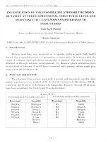
of this curve. The curve of composite waves (U L ) is defined as follows
(U L ) := W3→1 (U L ) ∪ W1→3 (U L ) ∪ W3→1→3 (U L ).

(3.1)

Thus, (U L ) has two endpoints I and U−0 = (h 0− , u 0− ) ∈ G −
2 (Fig. 1).
As mentioned above, the first part of (U L ), which is W3→1 (U L ) is an arc of the
curve W1 (U L0 ), and so it is strictly decreasing as written in the form u = u(h). The
third part of (U L ), which is W3→1→3 (U L ) is an arc of the hyperbola u/ h = positive
constant, so it is also strictly decreasing as written in the form u = u(h) as well. Now,
we consider the monotone property of the composite curve W1→3 (U L ). As seen in
Sect. 2, given a state U0 = (h 0 , u 0 ) at topography level a0 , the state U = (h, u) at
topography level a = a0 that can be connected to U0 by a stationary wave satisfies
the equations
F(h; U0 ) = 2gh 3 + (2g(a − a0 − h 0 ) − u 20 )h 2 + h 20 u 20 = 0,

123

u=

u0h0
. (3.2)
h

Properties of the Wave Curves in the Shallow Water...

315

Fig. 1 The composite wave curve (U L )

In view by Lemmas 2.2 and 2.3, the equation F(h; U0 ) = 0 could admit two roots
denoted by ϕ1 (U0 , a) and ϕ2 (U0 , a) such that
ϕ1 (U0 , a) < h 0 < ϕ2 (U0 , a) if a < a0 .
Moreover, as seen in Sect. 2, the Monotone Criterion selects ϕ2 (U0 , a) when U0 ∈
G 2 , and the state resulting from the stationary wave U = (h = ϕ2 (U0 , a), u =
u 0 h 0 /ϕ2 (U0 , a)) ∈ G 2 .
Now, let U0 vary on the curve W1 (U L )∩ G 2 , so we replace U0 by U1 (h) = (h, u =
w1 (U L ; h)) ∈ W1 (U L ) ∩ G 2 , at the topography level a L . In the sequel for simplicity
we write
w1 (h) = w1 (U L ; h), ϕ2 (h) = ϕ2 (U1 (h), a R ) where U1 (h) = (h, u = w1 (U L ; h)).
Then, the state on the other side of the admissible stationary wave from U1 (h) is
determined by
U10 (h) = (ϕ2 (U1 (h), a R ), u = w1 (h)h/ϕ2 (h)) ∈ G 2 .

123


316

M. D. Thanh, D. H. Cuong

Observe that ϕ2 (h) satisfying the equation
G(h) := F(h; U1 (h))

= 2gϕ23 (h) + 2g(a R − a L − h) − w12 (h) ϕ2 (h)2 + h 2 w12 (h) = 0. (3.3)

Lemma 3.1 Let U L ∈ G 1 ∪ C+ ∪ G +
2 , a L > a R , and let U1 (h) = (h, u =
w1 (U L ; h)) ∈ W1 (U L ) ∩ G 2 , where w1 is defined by (2.1), and (h ± , u ± ) ∈
W1 (U L ) ∩ C± . Then, the function ϕ2 (h) := ϕ2 (U1 (h), a R ) is strictly increasing for
h ∈ [h + , h − ].
Proof Differentiating (3.3) with respect to h, we get
0 = G (h) = 6gϕ22 (h)ϕ2 (h) + 2 2g(a R − a L − h) − w12 (h) ϕ2 (h)ϕ2 (h)
+ ϕ22 (h) −2g − 2w1 (h)w1 (h) + 2hw12 + 2h 2 w1 (h)w1 (h)
= ϕ2 (h)ϕ2 (h) 6gϕ2 (h) + 2 2g(a R − a L − h) − w12 (h)
+ 2 hw12 (h) − gϕ22 (h) + 2w1 (h)w1 (h) h 2 − ϕ22 (h) .

Then,
0 = ϕ2 (h)A + B,

(3.4)

where
A = ϕ22 (h) 3gϕ2 (h) + 2g(a R − a L − h) − w12 (h) ,
B = ϕ2 (h)

hw12 (h) − gϕ22 (h) + w1 (h)w1 (h) h 2 − ϕ22 (h)

From (3.4), to prove that ϕ2 (h) > 0, we need to show that
A > 0,

B < 0.

Indeed, it holds that

A = 3gϕ23 (h) − 2gϕ23 (h) + h 2 w12 (h)
= gϕ23 (h) − h 2 w12 (h)
> gh 3 − h 2 w12 (h) = h 2 gh − w12 (h) ≥ 0,
since U1 (h) = (h, w1 (h)) ∈ G 2 . This gives
A > 0.

123

.


Properties of the Wave Curves in the Shallow Water...

317

To prove that B < 0, we need to show that
θ (h) := w1 (h)w1 (h) ≥ −g, h + ≤ h ≤ h − .

(3.5)

Indeed, if w1 (h) < 0, then
θ (h) = w1 (h)w1 (h) > 0 > −g.
So, we remain to prove (3.5) for the case w1 (h) ≥ 0, i.e., h + ≤ h ≤ h , where h is
the h-intercept of the shock curve W1 (U L ). It holds that
d2
d
2w1 (h)w1 (h) = 2 w12 + w1 (h)w1 (h) > 0,
(w 2 (h)) =
dh 2 1
dh

for h + ≤ h ≤ h , since the curve W1 (U L ) is strictly convex. This implies that the
function θ (h) is increasing. So,
θ (h) ≥ θ (h + ) =

gh + w1 (h + ), h + ≤ h ≤ h .

(3.6)

We will show that
w1 (h + ) ≥ −

g
.
h+

Indeed, since the function w1 (h) is strictly convex, w1 (h) > 0, so w1 (h) is increasing.
That gives
w1 (h) > w1 (h ), h > h .
√
√ √
If h < h L , then w1 (h) = u L − 2 g h − h L . Thus,
w1 (h) = −
If h ≥ h L , then w1 (h) = u L −

g
2 (h

g
, h < hL.
h

− hL)

(h L , h) = w1 (h) − u L = −

1
h

+

1
hL

g
(h − h L )
2

(3.7)

. Set
1
1
.
+
h
hL

Then, it holds that
(h L , h) = − (h, h L ).

123


318

M. D. Thanh, D. H. Cuong

This yields
0 < −w1 (h) = −

h (h L , h)

=

h L (h, h L ),

so that
h L (h, h L )

≤

h L (h, h)

=

g
, h L ≤ h.
h

The last inequality yields

w1 (h) ≥ −

g
, h ≥ hL.
h

(3.8)

It follows from (3.7) and (3.8) that
w1 (h) ≥ −

g
, h+ ≤ h ≤ h .
h

Substituting the last inequality into (3.6) for h = h + , we get
θ (h) := w1 (h)w1 (h) ≥ θ (h + ) = − gh +

g
= −g, h + ≤ h ≤ h ,
h+

which establishes (3.5). Thus,
B = ϕ2 (h) hw12 (h) − gϕ22 (h) + w1 (h)w1 (h) h 2 − ϕ22 (h)
< ϕ2 (h) hw12 (h) − gϕ22 (h) + g ϕ22 (h) − h 2
= ϕ2 (h)h w12 (h) − gh < 0,
by (3.1) and U1 (h) = (h, w1 (h)) ∈ G 2 . Thus, A > 0, B < 0 and therefore
ϕ2 (h) =

d

ϕ2 (U1 (h), a R ) > 0.
dh

This terminates the proof of Lemma 3.1.
For the u-component of the composite wave curve, we have the following result.
Lemma 3.2 Consider the function u(h) = w1 (U L ; h)h/ϕ2 (U1 (h), a R ), where
U1 (h) = (h, u = w1 (U L ; h)) ∈ W1 (U L ) ∩ G 2 .
(a) If U L ∈ G 1 ∪ C+ and a L > a R , then the function u(h) is strictly decreasing for
h ∈ [h #L , h − ].
(b) If U L ∈ G +
2 and a L > a R , then the function u(h) is strictly decreasing for
h ∈ [h + , h − ].

123


Properties of the Wave Curves in the Shallow Water...

319

Proof First, consider the case w1 (h) ≥ 0, or h ∈ (h #L , h ), where h is the h-intercept
of the shock curve W1 (U L ). We will show that if U L ∈ G 1 ∪ C+ , then the function
f 1 (h) = w1 (h)h is strictly decreasing for h ∈ [h #L , h − ]. Actually, we have
√
f 1 (h) = u L −

√

It holds that
f 1 (h) = −

2g h L h + 4h 2 − h 2L
1
h

4hh L

+

1
hL

.

g/2 8h 3 + 12h 2 h L + 3hh L + h 3L
4h 3 h 3L

1
h

+

1
hL

3

(3.9)

(3.10)

˙ the function f in (3.10) is strictly decreasing on the
which is negative for h > 0So,
1
interval h ∈ (h #L , h ). The value f 1 (h # ) can be evaluated as follows:
f 1 h #L = u L −

2
2
2
g h L + 16u L /g − 3 h L + 8h L u L /g
.
8
uL

We will show that f 1 (h #L ) ≤ 0. Indeed, the condition
f 1 h #L ≤ 0
is equivalent to
u 2L ≤ gh L + 16u 2L − 3g h 2L + 8h L u 2L /g,
or
3g h 2L + 8h L u 2L /g ≤

g
h 2 + 8h L u 2L /g .
hL L

Simplifying the last inequality, we obtain
u L 2 ≥ gh L .
This shows that f 1 (h) < 0, h #L < h < h and so f 1 is strictly decreasing for h #L <
h

Similarly, we will show that if U L ∈ G 2 , then the function f 1 (h) = w1 (h)h is
strictly decreasing for h ∈ [h + , h ], where h is the h-intercept of the shock curve
W1 (U L ). Indeed, if U L ∈ G 2 , then w1 (h + ) = −

g
h+ ,

therefore

f 1 (h + ) = w1 (h + )h + + w1 (h + )
g
=−
h + + gh + = 0.
h+

123


320

M. D. Thanh, D. H. Cuong

Since f 1 (h) < 0, it implies that
f 1 (h) < 0, h + < h < h .
Thus, f 1 is strictly decreasing function for h + < h < h .
In both cases U L ∈ G 1 ∪ C+ and U L ∈ G 2 ,
u(h) = w1 (h)h

1
ϕ2 (U1 (h), h)

(3.11)

is the product of two positive and strictly decreasing functions of h #L < h < h and
h + < h < h , respectively, which is also strictly decreasing.
Second, we consider the case w1 (h) < 0. Observe that u(h) satisfying the equation
aL − a R +

1
w12 (h) − u 2 (h) + h − ϕ2 (h) = 0.
2g

Differentiating that equation with respect to h, we get
1
w1 (h)w1 (h) − u(h)u (h) + 1 − ϕ2 (h) = 0,
g
or
u(h)u (h) = w1 (h)w1 (h) + g − gϕ2 (h).
Multiplying both sides of the last equation by A and using (3.5), we get
u(h)u (h)A = w1 (h)w1 (h) + g A − g Aϕ2 (h)
= w1 (h)w1 (h) + g A + g B
= w1 (h)w1 (h) + g

gϕ23 (h) − h 2 w12 (h)

+ gϕ2 (h) hw12 (h) − gϕ22 (h) + w1 (h)w1 (h) h 2 − ϕ22 (h)
= w1 (h)w1 (h)h 2 gϕ2 (h) − w12 (h) + ghw12 (h) (ϕ2 (h) − h) > 0,
since w1 (h) < 0, ϕ2 (h) > h and U1 (h) = (h, w1 (h)) ∈ G 2 . Since A > 0 and
u(h) = w1 (h)h/ϕ2 (h) < 0, the last inequality implies that u (h) < 0 by (3.11). This
terminates the proof of Lemma 3.2.

Lemmas 3.1 and 3.2 yield the monotone property of the composite wave curve
W1→3 (U L ) as in the following theorem.
Theorem 3.3 If U L ∈ G 1 ∪ C+ and a L > a R , then the composite curve W1→3 (U L )
can be parameterized by h-component in the form u = u(h),
˜
h #L ≤ h ≤ h − , where
#
u = u(h)
˜
is strictly decreasing function of h L ≤ h ≤ h − .

123


Properties of the Wave Curves in the Shallow Water...

321

3.2 Case : U L ∈ G +
2 and a L > a R
From U L , the solution begins with a 1-rarefaction wave to a state U+ (h + , u + ) =
W1 (U L ) ∩ C+ . The solution is continued with a stationary wave from U+ (a L ) to the
state U+1 (a R ) ∈ G 1 using ϕ1 (U+ , a R ). There is one state U+1# ∈ W1 (U+1 ) such that
λ1 U+1 , U+1# = 0.
The solution is continued by a 1-wave from U+1 to state U such that 0 ≤ h ≤ h 1#
+ . The
set of U form the composite curve W1→3→1 (U L ). The composite curve W1→3→1 (U L )
is a part of the curve W1 (U+1 ). The curve W1 (U+1 ) intersects axis {h = 0} at the
point I = 0, u up := u 1+ + 2 gh 1+ . So, I and U+1# are two endpoints of the curve
W1→3→1 (U L ).

Again, let us denote by U± = (h ± , u ± ) the state at which the wave W1 (U L )
intersects with the curves C± , respectively. Then, from U L the Riemann solution can
begin with a 1-wave to state U ∈ W1 (U L )∩G 2 . This 1-wave is followed by a stationary
contact wave from state U (a L ) to a state U 0 (a R ) ∈ G 2 using ϕ2 (U, a R ). The set of
such a states U 0 forms a curve composite, denoted by W1→3 (U L ). Let U+0 and U−0 be
the two endpoints of this curve, i.e.,
U±0 = (h 0± , u 0± ) = (ϕ2 (U± , a R ), w3 (U± , ϕ2 (U± , a R ))) .

(3.12)

Besides, each level a ∈ [a R , a L ], from U L the Riemann solution can begin with the
1-rarefaction wave to U+ = W1 (U L ) ∩ C+ . This rarefaction wave can be followed
by a stationary contact wave from U+ (a L ) to a state M = M(a) ∈ G 1 ∪ C+ using
ϕ1 (U+ , a). The solution is continued with the 1-shock wave from the state M to the
state M # ∈ S1 (M) ∩ (G +
2 ∪ C+ ) such that
λ1 M, M # = 0.
Then, the solution is continued with the stationary contact wave from the state M # (a)
to the state M #0 (a R ) ∈ G 2 using ϕ2 (M # , a R ). The set of M #0 forms a curve composite,
denoted by W1→3→1→3 (U L ). If a = a R , then M = U+1 and M # = M #0 = U+1# . If
a = a L , then M = M # = U+ and M #0 = U+0 . So, U+1# and U+0 are two endpoints of
the curve composite W1→3→1→3 (U L ).
Let us define the composite wave curve
(U L ) = W1→3→1 (U L ) ∪ W1→3 (U L ) ∪ W1→3→1→3 (U L ).

(3.13)

Note that I and U−0 are the two endpoints of the curve (U L ).
Lemmas 3.1 and 3.2 provide us with the monotone property of the composite wave
curve W1→3 (U L ), as seen in the following theorem.

123


322

M. D. Thanh, D. H. Cuong

Fig. 2 The composite curve

(U L )

Theorem 3.4 If U L ∈ G +
2 and a L > a R , then the composite curve W1→3 (U L ) can be
˜
parameterized by h-component in the form u = u(h),
˜
h + ≤ h ≤ h − , where u = u(h)
is strictly decreasing function of h + ≤ h ≤ h − .
We have studied the curves of composite waves above in the case a R < a L above,
where composite waves are found in the form of combinations of 1-waves and stationary waves. When a R > a L , the construction will be relied on the backward wave
curve W2B (U R ). So, composite waves will be found as a combination of stationary
waves and backward 2-waves. The curve of these composite waves will be investigated
below (Figs. 2, 3).
3.3 Case : U R ∈ G 1 ∪ C+ ∪ G +
2 and a R > a L
At the right-hand state U R , the Riemann solution can arrive by a 2-wave from a state
U ∈ W2B (U R ) ∩ (G 2 ∩ C± ). Then, the Riemann solution is proceeded by a stationary
wave to U (a R ) from U 0 (a L ) ∈ G 2 using ϕ2 (U, a L ). The set of such states U 0 forms
B (U ). Let U 0 and U 0 denote the two endpoints

the backward composite curve W2←3
R
+
−
of this curve, where
U± = (h ± , u ± ) = W2B (U R ) ∩ C± ,
U±0 = (h 0± , u 0± ) = (ϕ2 (U± , a L ), w3 (U± , ϕ2 (U± , a L ))) .

123

(3.14)


Properties of the Wave Curves in the Shallow Water...

323

B (U )
Fig. 3 The composite curve W2←3
R

Similar to Lemma 3.1, we have following lemma.
Lemma 3.5 Let U R ∈ G 1 ∪ C+ ∪ G +
2 , a R > a L , and let U2 (h) = (h, u =
w2B (U R ; h)) ∈ W2B (U L ) ∩ G 2 , where w2B is defined by (2.1) and (h ± , u ± ) =
W1 (U L ) ∩ C± . Then, the function ϕ2 (h) = ϕ2 (U2 (h), a L ), h ∈ [h − , h + ] is strictly
increasing.
Proof The function ϕ2 (h) satisfies the equation
G(h) := F(h; U1 (h)) = 2gϕ23 (h)
2

2

+ 2g(a L − a R − h) − w2B (h) ϕ2 (h)2 + h 2 w2B (h) = 0.

(3.15)

0 = ϕ2 (h)A + B,

(3.16)

Therefore,
where
2

A = ϕ22 (h) 3gϕ2 (h) + 2g(a L − a R − h) − w2B (h) ,
B = ϕ2 (h)

2

hw2B (h) − gϕ22 (h) + w2B (h)w2B (h) h 2 − ϕ22 (h)

.

To establish the monotony of ϕ2 , we will show that
A > 0,

B < 0.

123

324

M. D. Thanh, D. H. Cuong

Indeed, it holds that
2

A = 3gϕ23 (h) − 2gϕ23 (h) + h 2 w2B (h)
2

= gϕ23 (h) − h 2 w2B (h)
2

2

> gh 3 − h 2 w2B (h) = h 2 gh − w2B (h) ≥ 0,
since U2 (h) = (h, w2B (h)) ∈ G 2 .
Next, to prove that B < 0, we need to show that
θ (h) := w2B (h)w2B (h) ≥ −g, h − ≤ h ≤ h + .

(3.17)

Indeed, if w2B (h) > 0, then
θ (h) = w2B (h)w2B (h) > 0 > −g.
So, we remain to prove (3.17) for the case w2B (h) ≤ 0. This means that h − ≤ h ≤ h ,
where h is the h-intercept of the backward curve W2B (U R ). It holds that
d
2

w2B (h)w2B (h) = w2B + w2B (h)w2B (h) > 0,
dh
for h − ≤ h ≤ h , since the curve W2B (U R ) is strictly concave. This implies that the
function θ (h) is increasing. So,
θ (h) ≥ θ (h − ) = − gh − w2B (h − ) = − gh −

g
= −g, h − ≤ h ≤ h . (3.18)
h−

which establishes (3.17). Thus,
2

B = ϕ2 (h) hw2B (h) − gϕ22 (h) + w2B (h)w2B (h) h 2 − ϕ22 (h)
2

< ϕ2 (h) hw2B (h) − gϕ22 (h) + g ϕ22 (h) − h 2
2

= ϕ2 (h)h w2B (h) − gh < 0,
by (3.17) and U2 (h) = (h, w2B (h)) ∈ G 2 . Thus, A > 0, B < 0 and therefore
ϕ2 (h) =

d
ϕ2 (U2 (h), a L ) > 0.
dh

This terminates the proof of Lemma 3.5.
Lemma 3.6 If U R ∈ G 1 ∪ C+ ∪ G +
2 and a R > a L , the function u(h) =

w2B (h)h/ϕ2 (U2 (h), a L ) is strictly increasing with respect to h ∈ [h − , h + ], where
U2 (h) = (h, u = w2B (U R ; h)) ∈ W2B (U R ) ∩ G 2 and w2B is defined by (2.1).

123


Properties of the Wave Curves in the Shallow Water...

325

Proof First, consider the case w2B (h) ≤ 0. We will show that the function f 2 (h) =
w2B (h)h is strictly increasing with respect to h ∈ [h − , h ]. Actually, since w2B (h) =
√
√ √
u R + 2 g h − h R , we have

f 2 (h) = w2B (h)h + w2B (h) =

g
h + w2B (h) =
h

gh + w2B (h).

(3.19)

It holds that
f 2 (h) =

1

2

g
+
h

3
g
=
h
2

g
,
h

which is positive for h > 0. So, the function f 2 is strictly increasing on the interval
h ∈ (h − , h ), where h is the h-intercept of the backward curve W2B (U R ). Moreover,
f 2 (h − ) =

gh − + w2B (h − ) =

gh − −

gh − = 0.

From (3.19), the last inequality shows that f 2 (h) > 0, h − < h < h and so f 2 is
strictly increasing for h − ≤ h ≤ h . Let us now consider the function
u(h) =

w2B (h)h
f 2 (h)
=
, h− ≤ h ≤ h .
ϕ2 (U1 (h), a L )
ϕ2 (h)

(3.20)

It holds that
u (h) =

f 2 (h)ϕ2 (h) − f 2 (h)ϕ2 (h)
ϕ22 (h)

> 0,

since ϕ2 (h) > 0, f 2 (h) > 0 and f 2 (h) < 0.
Next, we consider the case w2B (h) > 0. Observe that u(h) satisfying the equation
a R − aL +

1
2
w2B (h) − u 2 (h) + h − ϕ2 (h) = 0.
2g

Differentiating that equation with respect to h, we get
1
w2B (h)w2B (h) − u(h)u (h) + 1 − ϕ2 (h) = 0,
g

or
u(h)u (h) = w2B (h)w2B (h) + g − gϕ2 (h).

123


326

M. D. Thanh, D. H. Cuong

Multiplying both sides of the last equation by A and using (3.17), we get
u(h)u (h)A = w2B (h)w2B (h) + g A − g Aϕ2 (h)
= w2B (h)w2B (h) + g A + g B
= w2B (h)w2B (h) + g

2

gϕ23 (h) − h 2 w2B (h)

2

+ gϕ2 (h) hw2B (h) − gϕ22 (h) + w2B (h)w2B (h) h 2 − ϕ22 (h)
2

2

= w2B (h)w2B (h)h 2 gϕ2 (h) − w2B (h) + ghw2B (h)(ϕ2 (h) − h) > 0,
since w2B (h) > 0, ϕ2 (h) > h and U2 (h) = (h, w2B (h)) ∈ G 2 . Since A > 0 and
u(h) = w2B (h)h/ϕ2 (h) > 0 by (3.20), the last inequality implies that u (h) > 0. This
terminates the proof of Lemma 3.6.

From Lemmas 3.5 and 3.6, we obtain the monotonicity of the composite wave curve
B (U ) as follows.
W2←3
R

Theorem 3.7 If U R ∈ G 1 ∪ C+ ∪ G +
2 and a R > a L , then the composite curve
B (U ) can be parameterized by h-component in the form u = u(h),
˜
h− ≤ h ≤
W2←3
R
˜
is strictly increasing function of h − ≤ h ≤ h + .
h + , where u = u(h)

4 Deterministic Existence for the Riemann Problem
4.1 Case : U L ∈ G 1 ∪ C+ and a L > a R
Let us denoted by J = 0, w2B (U R , 0) the intersection point of the curve W2B (U R ) :
u = w2B (U R , h) and the u-axis. If w2B (U R , 0) < u up , then I = (0, u up ) is located
above the curve W2B (U R ). If u 0− < w2B (U R , h 0− ) then U−0 = (h 0− , u 0− ) is located below
the curve W2B (U R ). Whenever these two conditions are met, the backward wave curve
W2B (U R ) intersects the composite curve (U L ). This leads to the existence of solutions
of the Riemann problem, as stated in the following theorem.
Theorem 4.1 Let w2B and w3 be given by (2.1) and (2.13), respectively. Assume that
the left-hand state U L ∈ G 1 ∪ C+ , a L > a R , and the right-hand state U R satisfies
w2B (U R , 0) < u up ,
w2B (U R , h 0− ) > u 0− ,

(4.1)

where
u up = u 0L + 2 gh 0L ,
U L0 = (h 0L , u 0L ) = (ϕ1 (U L , a R ), w3 (U L , ϕ1 (U L , a R ))) ,
U− (h − , u − ) = W1 (U L ) ∩ C− ,
U−0 = (h 0− , u 0− ) = (ϕ2 (U− , a R ), w3 (U− , ϕ2 (U− , a R ))) .

123

(4.2)


Properties of the Wave Curves in the Shallow Water...

327

Then, the Riemann problems (1.1)–(1.2) has a solution.
Proof Let the curve (U L ) be parameterized as
h = h(m), u = u(m),
for m in some interval I . Since I, U−0 are the two endpoints of (U L ), we can assume
without loss of generality that I = [m 1 , m 2 ], where the values m 1 , m 2 are such that
I = (h(m 1 ), u(m 1 )) , and U−0 = (h(m 2 ), u(m 2 )) .
We define a function
G(m) := u(m) − w2B (U R , h(m)), m ∈ I.
it is easy to see that the function G(m) is continuous on I = [m 1 , m 2 ]. Moreover, it
holds that
G(m 1 ) = u(m 1 ) − w2B (U R , h(m 1 ))
= u up − w2B (U R , 0) > 0,
and
G(m 2 ) = u(m 2 ) − w2B (U R , h(m 2 ))

= u 0− − w2B (U R , h 0− ) < 0.
Therefore, there exists a value m 0 ∈ (m 1 , m 2 ) such that G(m 0 ) = 0, by IntermediateValue Theorem. This means that the curve (U L ) intersects the curve W2B (U R ) at
a point corresponding to m 0 , see Fig. 4. First, if the curve (U L ) intersects the part
W3→1 (U L ), then the Riemann problem has a solution of the form
W3 U L , U L0 ⊕ W1 U L0 , U ⊕ W2 (U, U R ).
Second, if the curve (U L ) intersects the part W3→1→3 (U L ), then the Riemann problem has a solution of the form
W3 U L , B ⊕ W1 B, B # ⊕ W3 B # , B #0 ⊕ W2 B #0 , U R .
Finally, if the curve (U L ) intersects the part W1→3 (U L ), then the Riemann problem
has a solution of the form
W1 U L , A ⊕ W3 A, A0 ⊕ W2 A0 , U R .
This completes the proof of Theorem 4.1.

123


328

M. D. Thanh, D. H. Cuong

Fig. 4 The composite curve (U L ) intersects the backward curve W2B (U R )

Consider the forward wave curve W2 (U0 ). A point is located above or below the curve
W2 (U0 ) can be characterized as in the following lemma.
Lemma 4.2 Given two states Ui = (h i , u i ), i = 1, 2. Then, u 1 < w2B (U2 , h 1 ) if
and only if u 2 > w2 (U1 , h 2 ). This means that a state U1 is located below the curve
W2B (U2 ) if and only if U2 is located above the curve W2 (U1 ) in the (h, u)-plane.
Proof The state U1 is located below the curve W2B (U2 ) means that
u 1 < w2B (U2 , h 1 ) ,
or
u1 <

√
√ √
u2 + 2 g h1 − h2 , h1 ≤ h2,
u2 +

g
2

(h 1 − h 2 )

1
h1

+

1
h2 ,

h1 > h2.

The last inequalities can be equivalently re-written as
u2 >

123

√
√ √
u1 + 2 g h2 − h1 , h2 ≥ h1,
u1 +

g
2

(h 2 − h 1 )

1
h2

+

1
h1 ,

h2 < h1,


Properties of the Wave Curves in the Shallow Water...

329

which means that
u 2 > w2 (U1 , h 2 ).
This completes the proof of Lemma 4.2.
As seen by Theorem 4.1, a large neighborhood of the left-hand state U L in which
the right-hand state U R can be chosen is obtained for the existence. It is interesting
that this region contains also large regions with simpler geometry such as triangles
and rectangles. This enables us to see more clearly the existence domain. Let us now
describe these regions. Since the curve W2 (U−0 ) is strictly concave, then the tangent
d of the curve W2 (U−0 ) at U−0 is always above the curve W2 (U−0 ). The tangent d is

given by
g
u = u bottom (h) := u 0− +
h − h 0− .
(4.3)
h 0−
The tangent d intersects the line u = u up , where u up is given by (4.2), in the (h, u)plane at a point with
h = h end := h 0− +

h 0−
u up − u 0− .
g

(4.4)

We define a triangle T as follows:
T = (h, u)| 0 < h < h end , u bottom (h) < u < u up ,

(4.5)

see Fig. 5.
Corollary 4.3 Assume that U L ∈ G 1 ∪ C+ , a L > a R . Then, U L ∈ T defined by (4.5),
and whenever U R ∈ T , the Riemann problem (1.1)–(1.2) has a solution.
Proof Since U R ∈ T , then U R is located above the tangent d, therefore, above the forward curve W2 (U−0 ). According to lemma 4.2, U−0 is located below the backward curve
√
W2B (U R ), therefore, u 0− < w2B (U R , h 0− ). Furthermore, w2B (0) = u R − 2 gh R <
u R < u up . According to theorem 4.1, the Riemann problem has a solution.
Now, we proof U L ∈ T . Since w1 (U L , h) is strictly decreasing function and U L ∈
G 1 , U− ∈ G 2 , then
0 < h L < h − < ϕ2 (U− , a R ) = h 0− < h end .

Other hand, since h 0L = ϕ1 (U L , a R ) < h L , then
u bottom (h L ) = u 0− +

g
uLhL
(h L − h 0− ) < 0 < u L <
0
h−
h 0L

= u 0L < u 0L + 2 gh 0L = u up .

123