DSpace at VNU: Acceleration of fast multipole method using special-purpose computer GRAPE
Bạn đang xem bản rút gọn của tài liệu. Xem và tải ngay bản đầy đủ của tài liệu tại đây (301.48 KB, 12 trang )
1
ACCELERATION OF FAST MULTIPOLE
METHOD USING SPECIAL-PURPOSE
COMPUTER GRAPE
1
Nguyen Hai Chau
2
Atsushi Kawai
3
Toshikazu Ebisuzaki
Abstract
We have implemented the fast multipole method (FMM) on
a special-purpose computer GRAPE (GRAvity piPE). The
FMM is one of the fastest approximate algorithms to calculate
forces among particles. Its calculation cost scales as O(N),
while the naive algorithm scales as O(N2). Here, N is the
number of particles in the system. GRAPE is hardware dedicated to the calculation of Coulombic or gravitational forces
among particles. GRAPE’s calculation speed is 100–1000
times faster than that of conventional computers of the same
price, though it cannot handle anything but force calculation.
We can expect significant speedup by the combination of the
fast algorithm and the fast hardware. However, a straightforward implementation of the algorithm actually runs on
GRAPE at rather modest speed. This is because of the limited functionality of the hardware. Since GRAPE can handle
particle forces only, just a small fraction of the overall calculation procedure can be put on it. The remaining part must
be performed on a conventional computer connected to
GRAPE. In order to take full advantage of the dedicated
hardware, we modified the FMM using the pseudoparticle
multipole method and Anderson’s method. In the modified
algorithm, multipole and local expansions are expressed by
distribution of a small number of imaginary particles (pseudoparticles), and thus they can be evaluated by GRAPE.
Results of numerical experiments on ordinary GRAPE systems show that, for large-N systems (N ≥ 105), GRAPE
accelerates the FMM by a factor ranging from 3 for low accuracy (RMS relative force error ~10–2) to 60 for high accuracy
(RMS relative force error ~10–5). Performance of the FMM
on GRAPE exceeds that of Barnes–Hut treecode on GRAPE
at high accuracy, in case of close-to-uniform distribution of
particles. However, in the same experimental environment
the treecode outperforms the FMM for inhomogeneous distribution of particles.
Key words: molecular dynamics, numerical simulation, fast
multipole method, tree algorithm, Anderson’s method, pseudoparticle multipole method, special-purpose computer.
Introduction
Molecular dynamics (MD) simulations are highly compute intensive. The most expensive part of MD is calculation of Coulombic forces among particles (i.e., atoms
and ions). In a naive direct-summation algorithm, cost of
the force calculation scales as O(N2), where N is the
number of particles. This is because Coulombic force is a
long-range interaction.
In order to reduce the cost of force calculation, fast
algorithms such as the Barnes–Hut treecode (Barnes and
Hut 1986) and the fast multipole method (FMM; Greengard and Rokhlin 1987) have been developed. In the treecode, particles are grouped and forces from them are
approximated by multipole expansions of the group. Particles that are more distant are organized into larger
groups, and thus the calculation cost scales as O(NlogN).
In the FMM, the force is also approximated by a multipole
expansion. Then the multipole expansion is converted to
a local expansion at each observation point. The force on
each particle is obtained by evaluating the local expansion. The calculation cost of this scheme scales as O(N).
These fast algorithms are widely used in the field of MD
simulation (Lakshminarasimhulu and Madura 2002;
Lupo et al. 2002).
There exists another approach to accelerate the force
calculation. It is to use hardware dedicated to the calculation of inter-particle forces. GRAPE (GRAvity PipE; Sugimoto et al. 1990; Makino and Taiji 1998) is one of the
most widely used pieces of special-purpose hardware of
this kind. Figure 1 shows the basic structure of a GRAPE
system. It consists of a GRAPE processor board and a
general-purpose computer (hereafter the host computer).
The host computer sends positions and charges of parti-
Fig. 1
Basic structure of a GRAPE system.
1
COLLEGE OF TECHNOLOGY, VIETNAM NATIONAL
UNIVERSITY, 144 XUAN THUY, CAU GIAY, HANOI, VIETNAM
(; )
2
K&F COMPUTING RESEARCH CO., 1-21-6-407,
KOJIMA-CHO, CHOFU, TOKYO, JAPAN 182-0026
3
The International Journal of High Performance Computing Applications,
Volume 22, No. 2, Summer 2008, pp. 194–205
DOI: 10.1177/1094342008090912
© 2008 SAGE Publications Los Angeles, London, New Delhi and Singapore
194
COMPUTATIONAL ASTROPHYSICS LABORATORY,
INSTITUTE OF PHYSICAL AND CHEMICAL RESEARCH,
(RIKEN), HIROSAWA 2-1, WAKO-SHI, SAITAMA,
JAPAN 351-0198
COMPUTING APPLICATIONS
Downloaded from hpc.sagepub.com at SETON HALL UNIV on March 30, 2015
cles to GRAPE. GRAPE then calculates the forces, and
sends results back to the host computer.
Using hardwired pipelines, a typical GRAPE system
performs the force calculation 100–1000 times faster
than conventional computers of the same price. For small5
N (say N <
∼ 10 ) particle systems, therefore, the combination of a simple direct-summation algorithm and GRAPE
is the fastest calculation scheme. Fast algorithms are not
very effective at such a small N.
For large-N particle systems, however, O(N2) directsummation becomes expensive, even with GRAPE. If we
successfully combine one of the fast algorithms and the
fast hardware, significant speed up for large-N particle
systems would be expected. As for the tree algorithm,
Makino (1991) has successfully implemented a modified
treecode (Barnes 1990) on GRAPE, and achieved a factor
of 30–50 speedup.
For the FMM, on the other hand, no implementation
on GRAPE so far exists. The FMM’s implementation on
dedicated hardware of a similar kind is reported, but its
performance is rather modest (Amisaki et al. 2003). This
is mainly because of the limited functionality of the hardware. Since dedicated hardware can calculate the particle
force only, it cannot handle multipole and local expansions. Therefore, only a small fraction of the FMM’s calculation can be performed on such hardware, and the
speedup gain remains rather modest.
In order to take full advantage of GRAPE, we modified the FMM using the pseudoparticle multipole method
(Makino 1999) and Anderson’s (1992) method. Using
these methods, we can express the multipole and local
expansion by a distribution of a small number of imaginary particles (pseudoparticles). With the modification, we
can use GRAPE to evaluate the expansions. Therefore, a
significant fraction of the modified FMM can be handled
on GRAPE.
In this paper we describe the implementation and performance of the modified FMM on GRAPE. The paper is
organized as follows. Section 2 gives a summary of the
FMM and related algorithms. In Section 3, a brief overview of GRAPE system is given. In Section 4, we describe
the implementation of our FMM code, which is modified
so that it runs on GRAPE. Results of numerical tests of the
code are shown in Section 6. Section 7 is devoted to discussion and Section 8 summarizes.
2
FMM and Related Algorithms
Here we give a brief description of the FMM (Section 2.1),
and two related algorithms, namely, the Anderson’s
method (Section 2.2) and the pseudoparticle multipole
method (Section 2.3). As will be seen in Section 4, the
latter two algorithms are used to implement the FMM on
GRAPE.
Fig. 2
2.1
Schematic idea of force approximation in FMM.
FMM
The FMM is an approximate algorithm to calculate
forces among particles. In case of close-to-uniform distribution of particles, the FMM’s calculation cost scales as
O(N). This scaling is achieved by approximation of the
forces using the multipole and local expansion technique.
Figure 2 shows a schematic idea of force approximation in the FMM. The force from a group of distant particles are approximated by a multipole expansion. At an
observation point, the multipole expansion is converted
to local expansion. The local expansion is evaluated by
each particle around the observation point. A hierarchical
tree structure is used for grouping of the particles.
The algorithm is applicable for two-dimensional (Greengard and Rokhlin 1987) and three-dimensional (Greengard
and Rokhlin 1997) particle systems. In the following, we
review the calculation procedure of the algorithm for the
three-dimensional case.
2.1.1 Tree construction Assume we have an isolated
particle system. Initially, we define a large enough cube
(root cell) to cover all particles in the system. We construct an oct-tree structure by hierarchical subdivision of
the cube into eight smaller cubes (child cells). The subdivision procedure starts from the root cell at refinement
level l = 0. The subdivision is then repeated recursively
for all sub cells, and stopped when l reaches an optimal
refinement level lmax. The optimal level lmax is determined
so that it optimizes the calculation speed.
2.1.2 M2M transition Next, we form multipole expansions for each leaf cell by calculating contributions from
all particles inside the cell.
Then we ascend the tree structure to form multipole
expansions of all non-leaf cells in all coarser levels. The
procedure starts from parents of the leaf cells. For each cell,
the multipole expansions of its children are shifted to the
geometric center of the cell (M2M transition) and summed.
This procedure is continued until it reaches the root cell.
ACCELERATION OF FMM USING GRAPE
Downloaded from hpc.sagepub.com at SETON HALL UNIV on March 30, 2015
195
2.2
Anderson’s Method
Anderson (1992) proposed a variant of the FMM using a
new formulation of the multipole and local expansions.
The advantage of his method is its simplicity. Anderson’s
method makes the implementation of the FMM significantly simpler. Here we briefly describe his method.
Anderson’s method is based on the Poisson’s formula.
This formula gives the solution of the boundary value
problem of the Laplace equation. When the potential on
the surface of a sphere of radius a is given, the potential
Φ at position →
r = (r, φ, θ) is expressed as
a n+1
1 ∞
s→⋅ →
r
→
→
( 2n + 1 ) --- P n --------- Φ ( as )ds (1)
Φ ( r ) = -----
r
4π S n = 0
r
∫∑
Fig. 3 Neighbour and interaction list of the hatched cell.
2.1.3 M2L conversion Then we evaluate the multipole
expansions. In order to describe this part, here we define
the terminology “neighbor list” and “interaction list.” The
neighbor list of a cell is a set of cells in the same level of
refinement which have contact with the cell. The interaction list of a cell is a set of cells which are children of the
neighbors of the cell’s parent and which are not neighbors
of the cell itself. Figure 3 shows the neighbor and interaction list of a cell for the two-dimensional case.
For each cell we evaluate the multipole expansion of
all cells in its interaction list. We convert the multipole
expansion to the local expansion at the geometric center
of the cell in question (M2L conversion), and sum them.
2.1.4 L2L transition In the next step, we descend the
tree structure. We sum the local expansions at different
refinement levels to obtain the total potential field at leaf
cells. For each cell in level l we shift the center of the
local expansion of its parent at level l – 1 (L2L transition), and then add it to the local expansion of the cell.
By this procedure, all cells in level l will have the local
expansion of the total potential field except for the contribution of the neighbor cells. By repeating this procedure for all levels, we obtain the potential field for all leaf
cells.
2.1.5 Force evaluation Finally, we calculate the force
on each particle in all leaf cells by summing the contributions of far field and near field forces. The near field contribution is directly calculated by evaluating the particle–
particle force. The far field contribution is calculated by
evaluating local expansion of the leaf cell at position of
the particle.
196
for r ≥ a, and
→ →
r n
1 ∞
s⋅r
→
→
( 2n + 1 ) --- P n --------- Φ ( as
Φ ( r ) = -----)ds
a
r
4π S n = 0
∫∑
(2)
for r ≤ a. Note that here we use a spherical coordinate
system. Here, Φ(a→
s ) is the given potential on the sphere
surface. The area of the integration S covers the surface
of the unit sphere centered at the origin. The function Pn
denotes the nth Legendre polynomial.
In order to use these formulae as replacements of the
multipole and local expansions, Anderson proposed a
discrete version of them, i.e., he truncated the right-hand
side of the equations (1)–(2) at a finite n, and replaced the
integrations over S with numerical ones using a spherical
t-design. Hardin and Sloane (1996) define the spherical tdesign as follows.
A set of K points 1 = {P1, …, PK} on the unit sphere
Ωd = Sd – 1 = {x = (x1, …, xd) ∈ Rd : x · x = 1} forms a
spherical t-design if the identity
∫ f ( x ) dµ ( x )
Ωd
1 K
f ( Pi )
= ---Ki = 1
∑
(3)
(where µ is a uniform measure on Ωd normalized to have
a total measure 1) holds for all polynomials f of degree ≤
t (Hardin and Sloane 1996).
Note that the optimal set, i.e., the smallest set of the
spherical t-design is not known so far for general t. In
practice we use spherical t-designs as empirically found
by Hardin and Sloane. Examples of such t-designs are available at />sphdesigns/.
Using the spherical t-design, Anderson obtained the
discrete versions of (1) and (2) as follows:
COMPUTING APPLICATIONS
Downloaded from hpc.sagepub.com at SETON HALL UNIV on March 30, 2015
→
Φ( r ) ≈
p
K
∑∑
i = 1n = 0
a
( 2n + 1 ) ---
r
n+1
s→i ⋅ →
r
- Φ ( as→i )w i (4)
P n -------- r
for r ≥ a (outer expansion) and
→
Φ( r ) ≈
p
∑∑
n
→
Qj =
(5)
for r ≤ a (inner expansion). Here wi is constant weight
value and p is the number of untruncated terms. Hereafter
we refer to p as the expansion order.
Anderson’s method uses equations (4) and (5) for
M2M and L2L transitions, respectively. The procedures
of other stages are the same as that of the original FMM.
2.3
p
N
→
i
s ⋅r
r
→
( 2n + 1 ) --- P n ---------- Φ ( as i )w i
a
r
i = 1n = 0
K
assigned to each pseudoparticle is then reduced from four
to one.
Makino’s approach systematically gives the solution
of the inversion formula as follows:
i
i=1
l
ij
),
(6)
l=0
where Qj is the charge of the pseudoparticle, →
r i = (ri, φ,
θ) is the position of the physical particle,
γ
is
the angle
ij
→
between →
r i and the position vector R j of the jth pseudoparticle. For the derivation procedure of equation (6),
see Makino (1999).
Equation (6) gives the solution for outer expansion.
We found that following a similar approach, we can
obtain the solution for inner expansion:
Pseudoparticle Multipole Method
Makino (1999) proposed the pseudoparticle multipole
method (P2M2) – yet another formulation of the multipole
expansion. The advantage of his method is that the expansions can be evaluated using GRAPE.
2 2
The basic idea of P M is to use a small number of
pseudoparticles to express the multipole expansions. In
other words, this method approximates the potential field
of physical particles by the field generated by a small
number of pseudoparticles. This idea is very similar to
that of Anderson’s method. Both methods use discrete
quantities to approximate the potential field of the original distribution of the particles. The difference is that
P2M2 uses the distribution of point charges, while Ander2 2
son’s method uses potential values. In the case of P M ,
the potential is expressed by point charges, and thus it
can be evaluated using GRAPE.
In the following, we describe the formulation procedure of P2M2.
The distribution of pseudoparticles is determined so
that it correctly describes the coefficients of a multipole
expansion. A naive approach to obtain the distribution is
to directly invert the multipole expansion formula. For a
relatively small expansion order, say p ≤ 2, we can solve
the inversion formula, and obtain the optimal distribution
with minimum number of pseudoparticles (Kawai and
Makino 2001).
However, it is rather difficult to solve the inversion
formula for higher p, since the formula is nonlinear. For
p > 2, we adopted Makino’s (1999) approach which is
more general. In his approach, pseudoparticles are fixed
at the positions given by the spherical t-design (Hardin
and Sloane 1996), and only their charges can change.
This makes the formula linear, although the necessary
number of pseudoparticles increases. This is because we
can adjust only the charges of pseudoparticles, since we
fixed the positions of them. The degree of freedom
l
2l + 1 r i
- --- P ( cos γ
∑ q ∑ ------------K a
p
N
Qj =
- ---
∑ q ∑ ------------K r
2l + 1 a
l+1
i
i=1
P l ( cos γ ij ).
(7)
i
l=0
For the derivation procedure of equation (7), see Appendix A.
3
Function of GRAPE
The
primary function of GRAPE is to calculate the force
→
f (→
i at position →
r i) exerted on particle
r i, and potential
→ →
→
φ( r i) associated with f ( r i). Although there are several
variants of GRAPE for different applications such as
astrophysics and MD, the basic functions of these hardware devices→are substantially the same.
→
The force f ( →
r i) and the potential φ( r i) are expressed as
→ →
i
f(r ) =
→
→
qj ( ri – rj )
--------------------3
rs
j=1
N
∑
(8)
and
→
φ ( ri ) =
N
qj
∑ ---r-,
j=1 s
(9)
where N is the number of particles to handle, →
r j and qj
are the position and the charge of particle j, and rs is the
softened distance between particle i and j defined as
2
2
→ 2
rs ≡ |→
r i – r j| + e , where e is →the softening parameter.
In order to calculate force f ( →
r i), relevant data, →
r i, →
r j,
qj, e, and N are sent from→the host computer to GRAPE.
GRAPE then calculates f ( →
r i) for every i, and sends it
back to the host. The potential φ( →
r i) is calculated in the
same manner.
4
Implementation of the FMM on GRAPE
The FMM consists of five stages (see Section 2.1),
namely, the tree construction, M2M transition, M2L con-
ACCELERATION OF FMM USING GRAPE
Downloaded from hpc.sagepub.com at SETON HALL UNIV on March 30, 2015
197
Table 1
Mathematical expressions and operations used in different implementations of the FMM.
Underlined parts run on GRAPE.
Original (Greengard and Rokhlin 1997)
M2M
Multipole expansion
M2L
M2L conversion formula
L2L
Local expansion
Near field force
Evaluation of physical-particle force
Far field force
Evaluation of local expansion
2
PM
Code B (Section 5)
2
P2M2
Evaluation of
pseudoparticle potential
Evaluation of
pseudoparticle potential
Anderson’s method
P 2 M2
Evaluation of
physical-particle force
Evaluation of
physical-particle force
Equation (10)
Evaluation of pseudo
particles force
version, L2L transition, and the force evaluation. The
force evaluation stage consists of near field and far field
evaluation parts.
In the case of the original FMM, only the near field
part of the force evaluation stage can be performed on
GRAPE. At this stage, GRAPE directly evaluates force
from each particle expressed in the form of equation (8).
At all other stages, mathematical operations not in the
form of equation (8) or equation (9) are required. GRAPE
cannot handle these operations.
In our implementation (hereafter code A), we modified
the original FMM so that GRAPE could handle the M2L
conversion stage, which is the most time consuming. For
2 2
this purpose, we used P M to express the multipole
expansions. With this modification GRAPE can handle
the M2L stage by evaluating potential values from the
pseudoparticles. At the L2L stage, potential values are
locally expanded and shifted using Anderson’s method.
Table 1 summarizes mathematical expressions and operations used at each calculation stage.
In the following, we describe the detail of our implementation.
reaches the root cell. This process is performed completely
on the host computer.
4.1 Tree Construction
4.6
The tree construction stage has no change. It is performed in the same way as in the original FMM.
Using equation (5), the far field potential on a particle at
position →
r can be calculated from the set of potential values
of the leaf cell which contains the particle. Meanwhile the far
field force is calculated using a derivative of equation (5):
4.2
M2M Transition
At the M2M transition stage, we compute positions and
charges of pseudoparticles, instead of forming multipole
expansion as in the original FMM.
The procedure starts from the leaf cells. Positions and
charges of the leaf cells are calculated from positions and
charges of physical particles. Then, those of non-leaf cells
are calculated from positions and charges of pseudoparticles of their child cells. This procedure is continued until it
198
Code A (Section 4)
4.3
M2L Conversion
The M2L conversion stage is done on GRAPE. In contrast to the original FMM we do not use the formula to
convert the multipole expansion to a local expansion. We
directly calculate potential values due to pseudoparticles
in the interaction list of each cell.
4.4
L2L Transition
The L2L transition is done in the same manner as Anderson. We use equation (5) to convert the local expansion
of each cell to that of its children.
4.5
Force Evaluation (Near Field)
The near field contribution is directly calculated by evaluating the particle–particle force. GRAPE can handle this
part without any modification of the algorithm.
Force Evaluation (Far Field)
→
– ∇Φ ( r ) ≈
ur→ – →
si r
→
nrP
n ( u ) + ------------------ ∇P n ( u )
2
i = 1n = 0
1–u
K
p
∑∑
r n – -2 →
g ( as i )w i,
× ( 2n + 1 ) -------an
where u = →
si · →
r /r.
COMPUTING APPLICATIONS
Downloaded from hpc.sagepub.com at SETON HALL UNIV on March 30, 2015
(10)
All the calculation at this stage is done on the host
computer.
5
Further Improved Implementation
With the modification described in Section 4, we have
successfully put the bottleneck, namely, the M2L conversion stage, on GRAPE. The overall calculation of the
FMM is significantly accelerated.
However, we still have room for improvement. The
M2L stage is put on GRAPE and is no longer a bottleneck. Now the most expensive part is the far field force
evaluation. Equation (10) is complicated and evaluation
of it would take rather a large fraction of the overall calculation time (Chau, Kawai, and Ebisuzaki 2002).
If we can convert a set of potential values into a set of
pseudoparticles at marginal calculation cost, the force
from those pseudoparticles can be evaluated on GRAPE,
and the bottleneck would disappear. In order to facilitate
this conversion, we have developed a new systematic
procedure (hereafter A2P conversion).
Using the A2P conversion, we have implemented yet
another version of FMM (hereafter code B). In code B,
we use A2P conversion to obtain a distribution of pseudoparticles that reproduces the potential field given by
Anderson’s inner expansion. Once the distribution of
pseudoparticles is obtained, the L2L stage can be performed using inner-P2M2 formula (equation (7)), and
then the force evaluation stage is totally done on GRAPE
(the final column of Table 1).
In the following, we show the procedure of A2P conversion.
For the first step, we distribute pseudoparticles on the
surface of a sphere with radius b using the spherical tdesign. Here, b should be larger than the radius of the
sphere a on which Anderson’s potential values g(a→
s i) are
defined. According to equation (7), it is guaranteed that
we can adjust the charge of the pseudoparticles so that
g(a→
s i) are reproduced. Therefore, the relation
K
Qj
∑ -------------------→
j=1
→
i
= Φ ( as→i )
R j – as
(11)
should
be satisfied for all i →= 1 … K. Using a matrix 1
=
→
→
→
T
{1/| R j – a s i|} and vectors Q = [Q1, Q2, …, QK] and P =
T
[Φ(a→
s 1), Φ(a→
s 2), …, Φ(a→
s K)], we can rewrite equation
(11) as
→
→
1Q = P.
(12)
In the next step, we solve the linear equation (12) to
obtain charges Qj. By numerical experiment we found
that appropriate value of radius b is about 6.0 for particles inside a cell with side length 1.0. Anderson (1992)
specified that a should be about 0.4. Because of large difference between a and b, equation (12) becomes nearly
singular for high order expansions. In this case, Gaussian
elimination and LU decomposition do not give a numerically accurate enough solution. Therefore, we applied
singular values decomposition (SVD; Press et al. 1992)
to solve the equation, and obtained better accuracy. The
additional cost for SVD is negligible.
6
Numerical Tests
We performed numerical tests on accuracy and performance of our hardware-accelerated FMM. Here we show
the results.
6.1 Accuracy of Inner-P2M2 and the A2P
Conversion
Here we show the result of a test on accuracy of the A2P
conversion (Section 5) and inner-P2M2 (equation (7)).
We performed the test in the following steps:
1. Locate a particle q at (r, π, π/2) (spherical coordinate). Here r runs from 1 to 10.
2. Evaluate potential values due to q at positions
defined by spherical t-design on the surface of a
sphere radius a = 0.4 centered at the origin. The
number and position of the evaluation points
depends on the expansion order p.
3. Apply A2P conversion to the local expansion
obtained in the previous step, i.e., solve equation
(12) to obtain charges of pseudoparticles Qj on the
surface of a sphere radius b = 6 centered at the origin. The number and position of the pseudoparticles depend on p.
4. Evaluate the force and potential due to the pseudoparticles at observation point L : (0.5, π, π/2).
5. Compare the result with exact force and potential.
The exact values are obtained by direct evaluation.
Figure 4 depicts the test process. Figures 5 and 6 show
the results of the test. The potential error and the force
error are shown in Figures 5 and 6, respectively. In both
cases, the error for p = 1 to 5 behaves as theoretically
expected, i.e., the potential error scales as r–(p + 2), and the
force error scales as r–(p + 1). For p = 6, the error stops
decreasing at r ≥ 6. This is because of the singularity of
the matrix 1 in equation (12). Since a large number of
pseudoparticles are used, the solution of equation (12)
suffers large computational error.
ACCELERATION OF FMM USING GRAPE
Downloaded from hpc.sagepub.com at SETON HALL UNIV on March 30, 2015
199
Fig. 6
Fig. 4 Description of the test for accuracy of innerP2M2 and the A2P conversion. Numbers on the figure
are steps in the test.
Fig. 5 Error of the potential calculated with inner2 2
P M and the A2P conversion. From top to bottom, six
dashed curves are plotted with expansion order p = 1,
2, 3, 4, 5 and 6, respectively.
6.2
Performance on MDGRAPE-2
Here we show the performance of the FMM code B (Section 5) measured on MDGRAPE-2 (Susukita et al. 2003).
MDGRAPE-2 is one of the latest devices in the GRAPE
series. It is developed for MD simulation and has additional function to the original GRAPEs, so that it can
2
handle forces that do not decay as 1/r , such as Van der
Waals force. However, in our test we use MDGRAPE-2
only to calculate Coulombic force and potential. The
additional functions are not used in our tests.
200
Force error: details as in Figure 5.
For the measurement, we used two GRAPE systems.
The first one consists of one MDGRAPE-2 board (64
pipelines, 192 Gflop/s) and a host computer COMPAQ
DS20E (Alpha 21264/667 MHz). The second one consists of one MDGRAPE-2 board (16 pipelines, 48 Gflop/s)
and a self-assembled host computer (Pentium 4/2.2 GHz,
Intel D850 motherboard). We refer the former system as
“system I,” and the latter as “system II.”
In the test, we distributed particles uniformly within a
unit cube centered at the origin, and evaluated the force
on all particles. The number of particles is from 128K to
4M. Notations K and M are 1024 and 1024 × 1024,
respectively. We measured the calculation time at both
high (p = 5) and low (p = 1) accuracy, with and without
GRAPE. The finest refinement level lmax is set to lmax = 4
and 5, for runs with and without GRAPE, respectively.
These values are experimentally chosen so that the overall calculation time is minimized (see Section 2.1).
In this paper we do not present in detail our experiments
in the case of inhomogeneous distribution of particles since
inhomogeneity is not as important as homogeneity or closeto-uniformity in molecular dynamics simulations. However,
our experiments in the two GRAPE systems show that the
treecode runs faster than the FMM in the inhomogeneous
case.
Results for close-to-uniform distribution cases are shown
in Figures 7–10 and Tables 2–3. Figures 7 and 9 are results
of system I. Figures 8 and 10 and Tables 2–3 are of system II.
In Figures 7 and 8, calculation time of the code B is
plotted against the number of particles N. Results shown
in Figures 7 and 8 are measured on system I and II,
respectively. Results of the direct-summation algorithm
are also shown for comparison. Our code scales as O(N)
2
while direct method scales as O(N ). On system I, runs
COMPUTING APPLICATIONS
Downloaded from hpc.sagepub.com at SETON HALL UNIV on March 30, 2015
Fig. 7 Force calculation time of FMM and direct-summation algorithm on system I. Circles denote performance of FMM on MDGRAPE-2. Pentagons denote that
on the host computer. Open and filled symbols are for
low (p = 1) and high accuracy (p = 5), respectively.
Solid and dashed curves without symbols are performance of direct method on MDGRAPE-2 and the host
computer, respectively.
Fig. 9 Comparison of force calculation time for FMM
and treecode on MDGRAPE-2 on system I. Circles are
performance of FMM on MDGRAPE-2. Triangles are
that of the treecode on MDGRAPE-2. Open and filled
symbols are for low and high accuracy, respectively.
Parameter pairs (p, θ) to obtain low and high accuracy
of the treecode are (1, 1.0) and (2, 0.33), respectively.
Fig. 8 Force calculation time of FMM and direct-summation algorithm on system II. Symbols as in Figure 7.
Fig. 10 Comparison of force calculation time for FMM
and treecode on MDGRAPE-2 on system II. Details as
in Figure 9.
with GRAPE are faster than those without GRAPE by a
factor of 5 and 60 for low (RMS relative force error ~10–2)
and high accuracy (RMS relative force error ~10–5),
respectively. On system II, the speedup factors are 3 and
14.5. Since the amount of calculation for the M2L stage
becomes more significant at higher p (Table 2), the speedup factor is larger for higher accuracy.
Table 3 shows the breakdown of the calculation time
for 1M-particle runs. We can see GRAPE significantly
accelerates the M2L part and force evaluation part. The
overall performance of our implementation is limited by
the speed of the communication bus between the host and
GRAPE, rather than the speed of GRAPE itself. For fur-
ACCELERATION OF FMM USING GRAPE
Downloaded from hpc.sagepub.com at SETON HALL UNIV on March 30, 2015
201
Table 2
Pairwise interaction count for 1M particle run.
With GRAPE
(lmax = 4)
Without GRAPE
(lmax = 5)
Low
High
Low
High
Accuracy
M2L
6.8 × 10
5
2.8 × 10
8
6
7.7 × 10
3.2 × 10⁹
Force evaluation
far field
1.6 × 10⁸
9.1 × 10⁹
1.8 × 10⁸
5.6 × 10⁹
near field
6.1 × 10⁹
6.1 × 10⁹
8.2 × 10⁸
8.2 × 10⁸
Table 3
Time breakdown for 1M particles run on system II.
With GRAPE
(lmax = 4)
Without GRAPE
(lmax = 5)
Low
High
Low
High
Tree construction
1.05
1.03
1.02
1.06
Building neighbor
and interaction lists
0.06
0.08
1.89
2.31
M2M
0.22
5.92
0.26
5.97
0.01
0.21
0.36
133.88
0.16
4.78
0
0
0.0004
0.18
0
0
_________
_________
_________
0.17
5.17
0.36
133.88
0.01
0.34
0.05
4.11
Host
0.78
0.97
54.35
330.99
Data transfer
8.57
17.37
0
0
Accuracy
M2L
Host
Data transfer
GRAPE
_____________________
L2L
_________
Force evaluation
GRAPE
_____________________
Total
3.92
9.48
0
0
_________
_________
_________
_________
13.27
27.82
54.35
330.99
14.78
40.36
57.93
478.32
ther acceleration, we need to switch from the legacy PCI
bus (32 bit/33 MHz) to the faster buses, such as PCI-X,
or PCI Express.
Figure 9 shows the calculation time of our FMM code
and the treecode (Kawai, Makino, and Ebisuzaki 2004),
both running on GRAPE. The order of the multipole
expansion p and the opening angle θ for the treecode is
set to (p, θ) = (1, 1.0) and (2, 0.33) for low and high accuracy, respectively. These values are chosen so that the
treecode gives roughly the same RMS force error as that
202
of the FMM. The RMS force errors at low and high accu–2
–5
racy are ~5 × 10 and ~2 × 10 , respectively.
We can see that the performance of our FMM code
and the treecode is almost the same. The FMM is better
than the treecode at high accuracy, and worse at low
accuracy.
In a particular GRAPE system, parameters tuning for
optimal performance of the modified FMM can be defined
by experiments. One should measure the code B’s performance on a randomly generated particles system with
COMPUTING APPLICATIONS
Downloaded from hpc.sagepub.com at SETON HALL UNIV on March 30, 2015
Table 4
Performance comparison with Wrankin’s code.
N
Wrankin’s
code
Our code
with
GRAPE
without
GRAPE
98,304
33.2
2.9
34.1
393,216
190.2
16.4
196.5
1,572,864
629.6
64.0
878.8
different values of the finest refinement level lmax for
each expansion order p from 1 to 5. For example, if the
number of particles in the system is from 128K to 4M
and the GRAPE’s peak performance is either 48 Gflop/s
or 192 Gflop/s then the values of lmax that should be
tested are 3, 4 and 5.
7
7.1
Discussion
Comparison with Other Implementations
We compared the performance of our FMM implementation (the code B) with Wrankin’s distributed parallel
multipole tree algorithm (DPMTA; Wrankin and Board
1995).
We measured the performance of Wrankin’s code on system II, using the serial version of DPMTA 3.1.3 available at
/>For the measurement, particles are distributed in a unit
cube. The expansion order and other parameters of each
code are chosen so that relatively high accuracy (~10–5)
is achieved, and the performance is optimized.
Table 4 summarizes the comparison. Using GRAPE,
our code outperforms Wrankin’s codes by tenfold. Without GRAPE, our code is slower than Wrankin’s code by a
factor of 1.1–1.4, mainly because our code requires a
larger number of operation counts, so that it takes full
advantage of GRAPE.
7.2
Kawai 2005). We can follow a similar approach to parallelize our FMM code.
Parallelization on GRAPE Cluster
Parallelization of the FMM on a cluster of GRAPEs
requires no special techniques. Algorithms used for parallelization on a cluster of general-purpose computers
(Hu and Johnsson 1996) can be applied without modification. In our modified FMM, GRAPE is used for the
M2L and force evaluation stages. The presence of
GRAPE has no effect to parallelization of the tree construction, building neighbor and interaction lists.
In the case of the treecode, several versions of parallel
codes have been developed so far. These codes are used
for productive runs in the field of astrophysics (Fukushige, Kawai, and Makino 2004; Fukushige, Makino, and
8
Summary
Using special-purpose hardware GRAPE, we have successfully accelerated the FMM. In order to take full
advantage of the hardware, we have modified the original
FMM using Anderson’s method, the pseudoparticle
multipole method, and two conversion techniques we
have newly invented. The experimental results show that
GRAPE accelerates the FMM by a factor of 3 to 60, and
the factor increases as the required accuracy becomes
higher. Comparison with the treecode shows that in the
case of close-to-uniform distribution of particles, our
FMM is faster at high accuracy, while the treecode is
faster at low accuracy. In case of inhomogeneous distribution of particles, the treecode is faster than the FMM.
It is suggested that one should use the code B for large
scale molecular dynamics simulations and where high
accuracy is demanded.
Acknowledgments
Thanks are due to Dr T. Iitaka at the Institute of Physical
and Chemical Research (RIKEN) for the suggestion of
using the SVD method.
We are grateful to Prof. J. A. Smith from Bridge to
Asia and Prof. D. E. Keyes from Columbia University for
refining the manuscript.
This work is supported by the Advanced Computing
Center, RIKEN and the College of Technology, Vietnam
National University, Hanoi. Part of this work was carried
out while N. H. Chau was a contract researcher of
RIKEN and A. Kawai was a special postdoctoral
researcher of RIKEN.
Appendix A
In this appendix, we describe the derivation procedure of
2 2
equation (7), inner expansion of P M .
The local expansion of the potential Φ( →
r ) is expressed as
→
p
Φ ( r ) = 4π
l
∑∑β
r Y l ( θ, φ ).
m l
l
m
(13)
l = 0 m = –l
Here, Y l (θ, φ) is the spherical harmonics and β l is the
expansion coefficient. In order to approximate the potential field due to the distribution of N particles, the coefficients should satisfy
m
m
1 N
1 m*
m
- Y ( θ i, φ i ),
β l = -------------- q i -------2l + 1 i = 1 r li + 1 l
∑
(14)
ACCELERATION OF FMM USING GRAPE
Downloaded from hpc.sagepub.com at SETON HALL UNIV on March 30, 2015
203
where qi and →
r i = (ri, θ, φ) are the charges and positions
of the particles, and * denotes the complex conjugate.
In order to reproduce the expansion→Φ( →
r ) up to pth
order, the charges Qj and the positions R j = (Rj, θj, φj) of
pseudoparticles must satisfy
In practice, we can directly calculate Qj from the charges
qi and the positions →
r i of physical particles.
Combining equations (14) and (19), Qj is expressed as
4π
Q j = -----K
p
N
l
∑ ∑ ∑ q r---
b
i
l = 0 m = –l i = 1
i
l+1
Y l ( θ j, φ j )Y l ( θ i, φ i ). (20)
m
m*
K
1
1 m*
m
- Y ( θ j, φ j )
β l = -------------- Q j --------2l + 1 j = 1 R lj + 1 l
∑
(15)
2
for all (p + 1) combinations of l and m in the range of 0 ≤
l ≤ p and –l ≤ m ≤ l. Here K is the number of pseudoparticles.
Following Makino’s (1999) approach, we restrict the
distribution of pseudoparticles to the surface of a sphere
centered at the origin. With this restriction, the coefficients of local expansion generated by the pseudoparticles are expressed as
K
1
m
- Q j Y m*
β l = ---------------------------l ( θ j, φ j ),
l+1
( 2l + 1 )b j = 1
∑
(16)
where b is the radius of the sphere. If we consider the
limit of infinite K, equation (16) is replaced by
1
- ρ ( a, θ, φ )Y m*
β = ---------------------------l ( θ, φ )ds.
l–1
( 2l + 1 )b S
∫
m
l
(17)
Here S is the surface of a unit sphere, and ρ is the continuous charge representation of pseudoparticle. In this
limit, the charge distribution is obtained by the inverse
transform of spherical harmonics expansion as follows:
p
ρ ( a, θ, φ ) =
l
∑ ∑ ( 2l + 1 )b
l–1
m
β l Y l ( θ, φ ).
m
(18)
l = 0 m = –l
We can discretize ρ using the spherical t-design. In other
words, the spherical t-design gives a distribution of pseudoparticles over which numerical integration retains the
orthogonality of spherical harmonics up to pth order. The
charges of the pseudoparticles are then obtained as
Using the addition theorem of spherical harmonics, we
can simplify this equation and obtain the formula to give
Qj from qj and →
r i:
p
N
Qj =
- ---
∑ ∑ ------------K r
qi
i=1
2l + 1 b
l=0
i
l+1
P l ( cos γ ij ).
(21)
Author Biographies
Nguyen Hai Chau, has a Ph.D. and his present position
is head of the Information Systems Department, Faculty
of Information Technology, College of Technology,
Vietnam National University, Hanoi, Vietnam (http://
www.coltech.vnu.edu.vn). Nguyen Hai Chau obtained his PhD degree in computer science from Vietnam
National University in 1999. His research interests are
fast algorithms for force calculation in molecular dynamics simulations and fuzzy reasoning methods.
Atsushi Kawai has a Ph.D. and is currently chief technical officer of K&F Computing Research Co. (http://
www.kfcr.jp/index-e.html). Atsushi Kawai obtained his PhD degree in computer science from Tokyo
University in 2000. His research interests are the development of special-purpose computers and software dedicated to scientific simulations.
Toshikazu Ebisuzaki has a Ph.D. and is currently chief
scientist of the Computational Astrophysics Laboratory,
RIKEN (). Toshikazu Ebisuzaki obtained his PhD degree in astrophysics from Tokyo
University in 1986. His research interests are: ultra-high
energy cosmic-rays; development of super-high speed
special-purpose computers; dynamics of biomolecules;
computational materials science; science of the earth and
planets; application of computers to education.
References
4π
Q j = -----K
p
l
∑ ∑ ( 2l + 1 )b
l+1
m
β l Y l ( θ j, φ j ).
m
(19)
l = 0 m = –l
This equation gives the charges Qj of pseudoparticles
m
from the expansion coefficients of physical particles β l .
204
Amisaki, T., Toyoda, S., Miyagawa, H., and Kitamura, K.
(2003). Development of hardware accelerator for molecular dynamics simulations: A computation board that calculates nonbonded interactions in cooperation with fast
multipole method, Journal of Computational Chemistry
24: 582–592.
COMPUTING APPLICATIONS
Downloaded from hpc.sagepub.com at SETON HALL UNIV on March 30, 2015
Anderson, C. R. (1992). An implementation of the fast
multipole method without multipoles, SIAM Journal on
Scientific and Statistical Computing 13(4): 923–947.
Barnes, J. E. (1990). A modified tree code: Don’t laugh; It runs,
Journal of Computational Physics 87: 161–170.
Barnes, J. E. and Hut P. (1986). A hierarchical O(NlogN) force
calculation algorithm, Nature 324: 446–449.
Chau, N. H., Kawai, A., and Ebisuzaki, T. (2002). Implementation of fast multipole algorithm on special-purpose computer MDGRAPE-2. In Proceedings of the 6th World
Multiconference on Systemics, Cybernetics and Informatics 2002 (SCI2002), Orlando, Colorado, USA, July 14–
18, pp. 477–481.
Fukushige, T., Kawai, A., and Makino, J. (2004). Structure of
dark matter halos from hierarchical clustering. III. Shallowing of the inner cusp, Astrophysical Journal 606: 625–
634.
Fukushige, T., Makino, J., and Kawai, A. (2005). GRAPE-6A:
A single-card GRAPE-6 for parallel PC-GRAPE cluster
systems, Publications of the Astronomical Society of
Japan 57: 1009–1021.
Greengard, L. and Rokhlin, V. (1987). A fast algorithm for particle simulations, Journal of Computational Physics 73:
325–348.
Greengard, L. and Rokhlin, V. (1997). A new version of the fast
multipole method for the Laplace equation in three dimensions, Acta Numerica 6: 229–269.
Hardin, R. H. and Sloane, N. J. A. (1996). McLaren’s improved
snub cube and other new spherical design in three dimensions, Discrete and Computational Geometry 15: 429–
441.
Hu, Y. and Johnsson, S. L. (1996). A data-parallel implementation of hierarchical N-body methods, International Journal of Supercomputer Applications and High Performance
Computing 10(1): 3–40.
Kawai, A. and Makino, J. (2001). Pseudoparticle multipole
method: A simple method to implement a high-accuracy
treecode, The Astrophysical Journal 550: L143–L146.
Kawai, A., Makino, J., and Ebisuzaki, T. (2004). Performance
analysis of high-accuracy tree code based on the pseudoparticle multipole method, The Astrophysical Journal
Supplement 151: 13–33.
Lakshminarasimhulu, P. and Madura, J. D. (2002). A cell
multipole based domain decomposition algorithm for
molecular dynamics simulation of systems of arbitrary
shape, Computer Physics Communications 144: 141–153.
Lupo, J. A., Wang, Z. Q., McKenney, A. M., Pachter, R., and
Mattson, W. (2002). A large scale molecular dynamics
simulation code using the fast multipole algorithm
(FMD): Performance and application, Journal of Molecular Graphics and Modelling 21: 89–99.
Makino, J. (1991). Treecode with a special-purpose processor,
Publications of the Astronomical Society of Japan 43:
621–638.
Makino, J. (1999). Yet another fast multipole method without
multipoles – Pseudoparticle multipole method, Journal of
Computational Physics 151: 910–920.
Makino, J. and Taiji, M. (1998). Scientific simulations with special-purpose computers – The GRAPE systems, Chichester: John Wiley and Sons.
Press, W. H., Teukolsky, S. A., Vetterling, W. T., and Flannery,
B. P. (1992). Numerical recipes in C – The art of scientific
computing, 2nd edition, Cambridge University Press,
New York, NY.
Sugimoto, D., Chikada, Y., Makino, J., Ito, T., Ebisuzaki, T., and
Umemura, M. (1990). A special-purpose computer for
gravitational many-body problems, Nature 345: 33–35.
Susukita, R., Ebisuzaki, T., Elmegreen, B. G., Furusawa, H.,
Kato, K., Kawai, A., Kobayashi, Y. et al. (2003). Hardware accelerator for molecular dynamics: MDGRAPE-2,
Computer Physics Communications 155: 115–131.
Wrankin, W. T. and Board, J. A. (1995). A portable distributed
implementation of the parallel multipole tree algorithm. In
Proceedings of the Fourth IEEE International Symposium
on High Performance Distributed Computing 1995
(HPDC 95), The Ritz Carlton Pentagon City, Virginia,
ACCELERATION OF FMM USING GRAPE
Downloaded from hpc.sagepub.com at SETON HALL UNIV on March 30, 2015
205