DSpace at VNU: An Approach for the Prediction of Optimum Conditions for the Steam Assisted Gravity Drainage Process by Response Surface Methodology
Bạn đang xem bản rút gọn của tài liệu. Xem và tải ngay bản đầy đủ của tài liệu tại đây (2.41 MB, 14 trang )
This article was downloaded by: [University of Calgary]
On: 03 September 2014, At: 23:33
Publisher: Taylor & Francis
Informa Ltd Registered in England and Wales Registered Number: 1072954 Registered
office: Mortimer House, 37-41 Mortimer Street, London W1T 3JH, UK
Energy Sources, Part A: Recovery,
Utilization, and Environmental Effects
Publication details, including instructions for authors and
subscription information:
/>
An Approach for the Prediction of
Optimum Conditions for the Steam
Assisted Gravity Drainage Process by
Response Surface Methodology
ab
a
a
H. X. Nguyen , T. B. N. Nguyen , W. Bae , T. Q. C. Dang
Chung
ac
& T.
a
a
Sejong University, Seoul, Korea
b
Ho Chi Minh City University of Technology, Ho Chi Minh, Vietnam
c
Department of Chemical and Petroleum Engineering, University of
Calgary, Calgary, Alberta, Canada
Published online: 26 Mar 2014.
To cite this article: H. X. Nguyen, T. B. N. Nguyen, W. Bae, T. Q. C. Dang & T. Chung (2014) An
Approach for the Prediction of Optimum Conditions for the Steam Assisted Gravity Drainage Process
by Response Surface Methodology, Energy Sources, Part A: Recovery, Utilization, and Environmental
Effects, 36:10, 1103-1114, DOI: 10.1080/15567036.2010.545796
To link to this article: />
PLEASE SCROLL DOWN FOR ARTICLE
Taylor & Francis makes every effort to ensure the accuracy of all the information (the
“Content”) contained in the publications on our platform. However, Taylor & Francis,
our agents, and our licensors make no representations or warranties whatsoever as to
the accuracy, completeness, or suitability for any purpose of the Content. Any opinions
and views expressed in this publication are the opinions and views of the authors,
and are not the views of or endorsed by Taylor & Francis. The accuracy of the Content
should not be relied upon and should be independently verified with primary sources
of information. Taylor and Francis shall not be liable for any losses, actions, claims,
proceedings, demands, costs, expenses, damages, and other liabilities whatsoever or
howsoever caused arising directly or indirectly in connection with, in relation to or arising
out of the use of the Content.
This article may be used for research, teaching, and private study purposes. Any
substantial or systematic reproduction, redistribution, reselling, loan, sub-licensing,
systematic supply, or distribution in any form to anyone is expressly forbidden. Terms &
Downloaded by [University of Calgary] at 23:33 03 September 2014
Conditions of access and use can be found at />
Energy Sources, Part A, 36:1103–1114, 2014
Copyright © Taylor & Francis Group, LLC
ISSN: 1556-7036 print/1556-7230 online
DOI: 10.1080/15567036.2010.545796
Downloaded by [University of Calgary] at 23:33 03 September 2014
An Approach for the Prediction of Optimum Conditions
for the Steam Assisted Gravity Drainage Process by
Response Surface Methodology
H. X. Nguyen,1;2 T. B. N. Nguyen,1 W. Bae,1 T. Q. C. Dang,1;3 and T. Chung1
1
Sejong University, Seoul, Korea
Ho Chi Minh City University of Technology, Ho Chi Minh, Vietnam
3
Department of Chemical and Petroleum Engineering, University of Calgary,
Calgary, Alberta, Canada
2
In this study, the application of response surface methodology and central composite design for
modeling the influence of some operating variables on the performance of steam-assisted gravity
drainage process for oil recovery was discussed. The maximized net present value of 105.16 $mm
was obtained when the optimum conditions of steam-assisted gravity drainage operation process was
designed following as injector/producer spacing of 5 m, injection pressure of 5,440 kPa, maximum
steam injection rate of 725 m3 /d, and spacing between two well pairs of 40 m. The predicted values
match the experimental values reasonably well, with R2 of 0.967 and Q2 of 0.82 for net present value
response.
Keywords: central composite design, net present value, response surface methodology, steam-assisted
gravity drainage
1. INTRODUCTION
Global conventional oil and natural gas reserves are on the decline. As a result, non-conventional
resources reservoirs, such as Alberta’s oil sand, are experiencing heightened global interest. Thus,
bitumen and heavy oil production are expected to increase rapidly in the coming decade. The
Athabasca Oil Sands are the center of this focus as one of the largest and highest-quality oil
sands resources in the world. An estimated 174 billion barrels of oil in the Athabasca deposit are
potentially recoverable with the present technology. Steam-assisted gravity drainage (SAGD) was
first developed by Roger Butler and his colleagues in Imperial Oil in the late 1970s (Butler, 2001).
SAGD is an effective method of producing heavy oil and bitumen, which consists of pairs of two
parallel horizontal wells drilled near the bottom of the pay. However, the process is associated
with high cost and high uncertainty if initial operating conditions design is unreasonable, it means
that the amount of oil recoverable or profit will be lower than actual production and even field
life can extend a long time. To overcome this situation, process engineers need to determine the
Address correspondence to Wisup Bae, Sejong University, 98 Gunja-dong, Gwangjin-ku, Seoul 143-747, Korea. E-mail:
Color versions of one or more of the figures in the article can be found online at www.tandfonline.com/ueso.
1103
Downloaded by [University of Calgary] at 23:33 03 September 2014
1104
H. X. NGUYEN ET AL.
levels of the operation design parameters at which the response reaches its optimum. The optimum
could be either a maximum or a minimum of an objective function of the design parameters. One
of the methodologies for obtaining the optimum results is response surface methodology (RSM)
(Myers and Montgomery, 1995).
In this study, the experimental design and response surface methodology was applied to mitigate
the risks and was aimed to obtain an optimal operating conditions design. The study investigates the
main four parameters for SAGD operation condition, including injector/producer spacing (IPS),
injection pressure (IP), maximum steam injection rate (MSIR), and spacing between two well
pairs (WPS), that affect the performance of SAGD operation as amount of oil recoverable and net
present value (NPV). It is essential that an experimental design methodology is very economical
for extracting the maximum amount of oil recoverable, a significant experimental time-saving
factor.
2. RESPONSE SURFACE METHODOLOGY
RSM is a statistical method based on the multivariate non-linear model that has been widely
used for optimization of the process variables of the operation process. Further, RSM consists of
designing experiments to provide adequate and reliable measurements of the response, developing
a mathematical model having the best fit to the data obtained from the experimental design,
and determining the optimal value of the independent variables that produce a maximum or
minimum response (Cornell, 1990; Montgomery, 2001; Myers and Montgomery, 2002; Myers
et al., 2008). The single-response modeled using the RSM corresponded to independent variables.
By the RSM, a quadratic polynomial equation was developed to predict the response as a function
of independent variables involving their interactions (Box and Draper, 1987). In general, the
response for the quadratic polynomial is described in Eq. (1):
Y D ˇ0 C
k
X
i D1
ˇi Xi C
k
X
i D1
ˇi i Xi2 C
X
ˇij Xi Xj C ";
(1)
i
where Y is the predicted response, ˇ0 the intercept coefficient, ˇi the linear terms, ˇi i the squared
terms, ˇij the interaction terms, and xi and xj represent the coded independent variables. In this
study, a second-order polynomial equation was obtained using the uncoded independent variables
as such:
Y D ˇ0 C ˇ1 X1 C ˇ2 X2 C ˇ3 X3 C ˇ4 X4 C ˇ11 X12 C ˇ22 X22 C ˇ33 X32 C ˇ44 X42
(2)
C ˇ12 X1 X2 C ˇ13 X1 X3 C ˇ14 X1 X4 C ˇ23 X2 X3 C ˇ24 X2 X4 C ˇ34 X3 X4 :
The coefficient of the model for the response was estimated using a multiple regression analysis
technique included in the RSM. Fit quality of the models was judged from their coefficients of
correlation and determination.
3. DESIGN OF EXPERIMENT USING CENTRAL COMPOSITE DESIGN
The experimental design techniques commonly used for process analysis and modeling are the full
factorial, partial factorial, and central composite rotatable designs. An effective alternative to the
factorial design is the central composite design (CCD), originally developed by Box and Wilson
and improved upon by Box and Hunter in 1957. The CCD gives almost as much information as
OPTIMUM CONDITIONS FOR SAGD
1105
a three-level factorial, requires much fewer tests than the full factorial, and has been known to be
sufficient to describe the majority of steady-state process responses.
Currently, CCD is the most popular class of designs used for fitting second-order models. The
total number of tests required for CCD is 2k C 2k C n0, including the standard 2k factorial points
with its origin at the center, 2k points fixed axially at a distance, say ˇ.ˇ D 2k=4 /, from the center
to generate the quadratic terms, and replicate tests at the center .n0/, where k is the number of
independent variables.
Downloaded by [University of Calgary] at 23:33 03 September 2014
3.1. Experiment Design for SAGD Operating Conditions
Two-dimensional numerical simulations were performed with a grid cell (101 1 m in the lateral
direction and 25 m thickness in the vertical direction) with CMG’s STARS using the petrophysical
parameters of the Athabasca reservoirs as described in the previous literatures (Shin and Polikar,
2005). The SAGD simulation model in the present application considered two well pairs parallel,
horizontal wells of 900 m length, oriented in the j direction, within a reservoir of McMurray
formation is located in shallow depth regions from 200 to 210 m, with no dip and 1,500 kPa
of initial pressure. The dimensions of each block were 1 m in i and k directions and 900 m in
the j direction. Constant values of porosity (35%) and directional permeability (Kv D 5d and
Kh D 2:5d ) were considered through the entire reservoir. The initial temperature was 18ı C and
all thermal properties of rock and fluids were the same for all runs, except the rock thermal
conductivity. All surfaces of the model have a no-flow boundary, but heat loss is assumed at the
overburden. No aquifer or gas cap zones were considered. A three-phase fluid model was assumed
to account for the methane content in the oil. Steam at 95% quality was injected at 265ıC.
The net present value over a period of 10 years of production was selected as the variable to
measure the SAGD production performance, and therefore, the dependent variable in the proposed
surface response correlation. This selection was done based on the comparison of the NPV with
the cumulative (CSOR) and instantaneous steam-to-oil ratio (ISOR), two common measurements
of SAGD performance. It can be seen that the maximum value of NPV coincides with the value
of SOR equal to four, considered as the limit value of maximum profitability. Above this limit,
the project is assumed not to be cost-effective (Shin and Polikar, 2005).
The design of the economic model was based on the one discussed in the Canadian National
Energy Board reports (2006, 2008). The economic model was a simplified cash flow model in an
Excel spreadsheet that included depreciation and a typical Alberta’s fiscal regime. All simulation
cases were run over a period of 10 years, and the result of the yearly cumulative oil production and
steam injection was the base to calculate the yearly income. The NPV was calculated considering
only the average price of bitumen ($60/bbl) and gas price 4.71$/GJ at an interest rate of 10%
a year. Drilling and completion costs of a well pair (2.5 $mm) were also considered as capital
investments. The production estimate is matched with investment and operating costs and rates of
return on capital to calculate the NPV.
The experimental design selected in this application is the central composite design (CCD) to
determine the relationship between four operating variables of the SAGD process, namely, spacing
between injector/producer (IPS), injection pressure (IP), maximum steam injection rate (MSIR),
and SAGD well pattern spacing (WPS). The number of tests at the center points was three, making
the total number of tests required for the four independent variables: 24 C .2 4/ C 3 D 27.
The injector/producer spacing .X1/, injection pressure .X2/, maximum steam injection rate
.X3/, and well pairs pattern spacing .X4/ were independent variables studied to predict Y
responses (net present value). The four independent variables and their levels for the CCD used
in this study are shown in Table 1. Using the relationships in Table 1, coded and actual levels
of the variables for each of the experiments in the design matrix were calculated as given in
Table 2. Based on this table, the experiments were conducted for obtaining the response, i.e.,
1106
H. X. NGUYEN ET AL.
TABLE 1
Four Independent Variables and Their Levels for CCD
Coded Variable Level
Downloaded by [University of Calgary] at 23:33 03 September 2014
Variable
Injector/producer spacing (IPS), m
Injection pressure, kPa
Max steam injection rate (m3 /d)
Well pairs pattern spacing (m)
Symbol
Low
1
Center
0
High
C1
X1
X2
X3
X4
5
2,500
360
40
10
5,500
600
70
15
8,500
840
100
TABLE 2
Independent Variables and Result for SAGD Operation Design by Central Composite Design
Coded Level
of Variables
Run
1
2
3
4
5
6
7
8
9
10
11
12
13
14
15
16
17
18
19
20
21
22
23
24
25
26
27
Actual Level
of Variable
X1
X2
X3
X4
1
1
1
1
1
1
1
1
1
1
1
1
1
1
1
1
1
1
0
0
0
0
0
0
0
0
0
1
1
1
1
1
1
1
1
1
1
1
1
1
1
1
1
0
0
1
1
0
0
0
0
0
0
0
1
1
1
1
1
1
1
1
1
1
1
1
1
1
1
1
0
0
0
0
1
1
0
0
0
0
0
1
1
1
1
1
1
1
1
1
1
1
1
1
1
1
1
0
0
0
0
0
0
1
1
0
0
0
Response
(Simulation Observed)
IPS, m
IP, kPa
MSIR, m3 /d
WPS, m
NPV, $mm
5
15
5
15
5
15
5
15
5
15
5
15
5
15
5
15
5
15
10
10
10
10
10
10
10
10
10
2,500
2,500
8,500
8,500
2,500
2,500
8,500
8,500
2,500
2,500
8,500
8,500
2,500
2,500
8,500
8,500
5,500
5,500
2,500
8,500
5,500
5,500
5,500
5,500
5,500
5,500
5,500
360
360
360
360
840
840
840
840
360
360
360
360
840
840
840
840
600
600
600
600
360
840
600
600
600
600
600
40
40
40
40
40
40
40
40
100
100
100
100
100
100
100
100
70
70
70
70
70
70
40
100
70
70
70
98.55
65.932
94
93.288
103.307
67.956
99.68
95
72.442
54.604
73.16
71.186
81.178
60.446
76.76
76.168
100.428
91.149
89.793
86.882
87.931
101.634
101.501
81.465
98.265
98.265
98.265
OPTIMUM CONDITIONS FOR SAGD
1107
NPV is carried out at the corresponding independent variables addressed in the experimental
design matrix. These experimental data are used for validating the single-response model of the
operation process. The sequence of the experiment was randomized in order to minimize the
effects of uncontrolled factors.
Downloaded by [University of Calgary] at 23:33 03 September 2014
4.
RESPONSE SURFACE METHODOLOGY EVALUATION
When fitting the model, various statistical analysis techniques were employed to judge the experimental error, the suitability of the model, and the statistical significance of the terms in the
model. This is usually done with the help of a computer, using either a statistics package or a
dedicated RSM program. In the present work, the adequacy of the model was justified through
analysis of variance (ANOVA).
The quality of the model is measured through statistics as R2, R2adj, and Q2. The coefficient
of multiple determination, R2, measures the percentage of variability observed on the response and
explained by the regression. It depends on the model and it will increase when adding more terms
to it. For this reason, it is not a suitable statistic for comparing models. An adjusted coefficient
R2adj is defined as being able to compare the different possible models. Any model with a value
of R2 and R2adj close to 1, indicates an excellent quality in fitting the observed data, but it does
not give any information about its power of prediction between the available data points.
In some cases, models that fit the experimental data properly are not good predictors. In order to
measure the power of prediction of a model, the statistic, Q2, is computed based on the prediction
sum of squares (PRESS). PRESS is then computed as the squared differences between observed Y
and predicted values Ypred. The minimization of PRESS leads to an improvement on the power
of prediction of the model. Once the model is constructed, it can be used to predict reservoir
performance and to optimize controllable variables (Vanegas Prada and Cunha, 2008).
5. RESULTS AND DISCUSSION
Response surface optimization is more advantageous than the traditional single parameter optimization in that it saves time, space, and injection raw material. There were a total of 27 cases
for optimizing the four individual parameters in the current CCD. Table 2 shows the experimental
conditions and the results of NPV according to the factorial design. Maximum NPV (103.307
$mm) was recorded under the experimental conditions of the injector/producer spacing, 5 m;
injection pressure, 2,500 psi; maximum steam injection rate, 840 m3 /d; and well pairs pattern
spacing, 40 m. By applying multiple regression analysis on the experimental data, the response
variable and the test variables were related by the following second-order polynomial equation:
Y D 97:35
6:88X1 C 3:995X2 C 2:83X3
9:54X4
0:51X1X3 C 2:01X1X4
8:55X2X2
2:11X3X3 C 0:56X3X4
5:41X4X4:
1:1X1X1
0:34X2X3
6:16X1X2
1:1X2X4
(3)
The results of the analysis of variance, goodness-of-fit, and the adequacy of the models are
summarized in Table 3. The determination coefficient (R2 D 0.967) was showed by ANOVA
of the quadratic regression model, indicating that only 3.3% of the total variations were not
explained by the model. The value of the adjusted determination coefficient (Adjusted R2 D
0.93) also confirmed that the model was highly significant. At the same time, a very low value
1108
H. X. NGUYEN ET AL.
Downloaded by [University of Calgary] at 23:33 03 September 2014
TABLE 3
ANOVA Analysis
NPV
DF
SS
MS
Total
Constant
Total corrected
Regression
Residual
Lack of fit
Pure error
N D 27
DF D 12
27
204,409
1
199,217
26
5,192.64
14
5,022.48
12
170.164
10
170.164
2
2.97e-012
Q2 D 0.82
R2 D 0.967
R2 Adj. D 0.93
F
p
7,570.72
199,217
199.717
358.748
25.299
14.1803
17.0164
1.48e-012
Cond. no. D 6.6122
Y-miss D 0
RSD D 3.766
0.000
SD
14.1321
18.9407
3.76568
4.125
1.22e-006
(3.76) of residual standard deviation (RSD) clearly indicated a very high degree of precision and
a good deal of reliability of the experimental values. The model was found to be adequate for
prediction within the range of experimental variables and especially the one related to the power
of prediction, Q2 D 0.82.
The regression coefficient values of Eq. (3) are listed in Table 4. The P-values were used as
a tool to check the significance of each coefficient, which in turn may indicate the pattern of the
interactions between the variables. The smaller was the value of P, the more significant was the corresponding coefficient. It can be seen from this table that the linear coefficients .X1; X2; X3; X4/,
a quadratic term coefficient .X22 ; X42 /, and cross product coefficients .X1:X2; X1:X4/ were
highly significant, with very small P-values .P < 0:05/. The other term coefficients were not
significant .P > 0:05/. The full model filled Eq. (3) made three-dimensional and contour plots
to predict the relationships between the independent variables and the dependent variables.
TABLE 4
Regression Coefficients of the Predicted Quadratic Polynomial Model
Standard
Error
NPV
Estimate
Constant
X1
X2
X3
X4
X1.X1
X2.X2
X3.X3
X4.X4
X1.X2
X1.X3
X1.X4
X2.X3
X2.X4
X3.X4
97.35
1.3877
6.87644
0.887579
3.99534
0.887579
2.83534
0.887579
9.54472
0.887578
1.10405
2.34831
8.55504
2.34831
2.11004
2.34831
5.40954
2.34831
6.16131
0.941419
0.51331
0.941419
2.01407
0.941419
0.33656
0.941419
1.10119
0.941419
0.561685
0.941419
Confidence level D 95%
P
4.68E-17
5.21E-06
0.000725
0.007711
1.62E-07
0.64668
0.003369
0.386576
0.039937
2.75E-05
0.59557
0.050021
0.726923
0.264826
0.561837
OPTIMUM CONDITIONS FOR SAGD
1109
Downloaded by [University of Calgary] at 23:33 03 September 2014
5.1. Main and Interaction Effect Plots
The main effect plot is appropriate for analyzing data in a designed experiment, with respect to
important factors, where the factors are at two or more levels. Figure 1 shows the effect plots
of variables on NPV, respectively. This graph could be divided into two regions, the region with
below to zero, where the factors and their interactions presented negative coefficients (WPS.WPS,
WPS, IPS, IP.IP, IPS.IPS, MSIR.MSIR) indicating NPV decrease and the region with above zero,
where the factors presented positive coefficients (MSIR, IPS.IP,IP, MSIR.WPS) indicating NPV
increase.
By analyzing the graph of Figure 1 and the values of Table 4, it can be inferred that the well
pattern spacing (WPS) was the most important variable of operating condition effect strongest on
NPV. The increase in spacing between two well pairs led to a remarkable decrease of NPV
because ultimate bitumen recovery decreases rapidly. Narrower well pattern spacing will be
more economical in SAGD operation. The second important factor for overall optimization of
an operating condition is injector producer spacing; an increase of IPS leads to decrease the NPV
(Figures 1 and 2a). The third important factor is injection pressure, when increase of IP leads to
increase slightly the NPV (Figures 1 and 2c).
5.2. Optimization of Operating Conditions for SAGD Process
The full model filled Eq. (3) was made three-dimensional and contour plots to predict the relationships between the independent variables and the dependent variables. The graphical representations
called the response surfaces, and the contour plots obtained the results of NPV affected by the
injector/producer spacing, injection pressure, maximum steam injection rate, and well pairs pattern
spacing (presented in Figures 3 and 4).
In the two figures, the maximum predicted value indicated by the surface was confined in
the smallest ellipse in the contour diagram. Elliptical contours are obtained when there is a
perfect interaction between the independent variables. The independent variables and maximum
FIGURE 1
The degree of factors effect on NPV.
Downloaded by [University of Calgary] at 23:33 03 September 2014
1110
H. X. NGUYEN ET AL.
FIGURE 2
Main factors effect on NPV.
FIGURE 3 Contour plot (2-D) showing the effects of variables on NPV.
Downloaded by [University of Calgary] at 23:33 03 September 2014
OPTIMUM CONDITIONS FOR SAGD
FIGURE 4
1111
Response surface plots (3-D) showing the effects of variables on NPV.
predicted values from the figures corresponded with the optimum values of the dependent variables
(responses) obtained by the equations.
The contour plot and the 3-D response surface plot of the NPV showed that the region of
maximized NPV can increase over 104 $mm with operating conditions, which injector/producer
spacing in the range of 5–8 m and the broad change of injection pressure from 2,500 to 7,800
kPa (Figures 3a, 3b, 3c, 4a, 4b, 4c). However, comparing three cases shows that the red smallest
ellipse area is found as an optimization area (Figure 3a), where the maximize NPV reaches over
104 $mm while IPS range of 4–5 m, injection pressure change slight from 4,000 to 6,500 kPa,
and the volume of steam injection at the lowest level 360 m3 /d, respectively.
At fixed well pattern spacing of 70 m in Figures 3d, 3e, 3f, 4d, 4e, and 4f indicated that
the maximum NPV can be achieved over 104 mm$ with injection pressure of 4,000–6,000 kPa,
but requires the use of larger quantities of steam injection at 840 m3 /d. Therefore, this case will
be uneconomical when compared with the case mentioned above. If beyond this level, the NPV
decreased with increasing injector/producer spacing.
When the well pattern spacing raises up 100 m, it indicates that the maximum NPV can only
reach lower at the yellow region (88.6 mm$, Figure 3i), where IPS is about 5 m and the injection
pressure changes from 4,000 to 5,000 kPa, respectively. It can be seen that the NPV in this case
is lowest or infeasible. This design should not be applied to optimize the operating condition for
SAGD process.
As shown in Figures 3 and 4 and Table 5, it can be concluded that maximization NPV of
operating condition design will be calculated by spacing between injector/producer spacing, 5 m;
injection pressure, 5,440 kPa; maximum steam injection rate, 725 m3 /d; and well pairs spacing,
40 m (Figure 5). Among the four parameters studied was the most significant factor to affect the
NPV according to the regression coefficients significance of the quadratic polynomial model and
gradient of slope in the 3-D response surface plot.
1112
H. X. NGUYEN ET AL.
TABLE 5
Predicted and Experimental Values of the Responses at Optimum Conditions
IPS, m
Downloaded by [University of Calgary] at 23:33 03 September 2014
5
Injection
Pressure,
kPa
Max.
Steam,
m3 /d
Well
Pattern
Spacing,
m
NPV,
$mm,
Predicted
NPV,
$mm,
Simulation
Difference,
%
5,440
725
40
110.166
105.164
4.54
FIGURE 5
Design of optimal location and operating conditions of SAGD well pairs in reservoir.
5.3. Verification of Predictive Model
The suitability of the objective equation for predicting optimum response values was tested
under the operating conditions for injector/producer spacing, 5 m; injection pressure, 5,400 kPa;
maximum steam injection rate, 725 m3 /d; and well pairs spacing, 40 m. This set of conditions
was determined to be optimum by the RSM optimization approach and was used to validate
experimentally and predict the values of the responses using the model equation. The total of
cumulative oil produced from the reservoir is about 600,000 m3 . However, in the second year,
the oil production rate rapidly decreased until the steam oil rate increased over 4.0 at the third
year (Figures 6 and 7). These outcomes are sent to an economic model to account for a NPV
of 105.164 $mm, demonstrating the validation of the RSM model, indicating that the model was
adequate for the SAGD operation process (Table 5).
6. CONCLUSIONS
The factors of operating conditions have significant effects on the NPV. Using the contour and
surface plots in RSM was effective for estimating the effect of four independent variables. The
Downloaded by [University of Calgary] at 23:33 03 September 2014
OPTIMUM CONDITIONS FOR SAGD
FIGURE 6
FIGURE 7
Oil recoverable at optimal condition.
Prediction production of SAGD performance at optimal condition.
1113
1114
H. X. NGUYEN ET AL.
Downloaded by [University of Calgary] at 23:33 03 September 2014
optimal set of the independent variables was obtained graphically in order to get the desired
levels of bitumen recovery. The maximize NPV of 105.164 $mm was obtained when the optimum
conditions of SAGD process were injector/producer spacing, 5 m; injection pressure, 5,440 kPa;
maximum steam injection rate, 725 m3 /d; and well pairs pattern spacing, 40 m. Under these
optimized conditions, the experimental purity of NPV agreed closely with the predicted yield of
4.54% (Table 5).
This study demonstrates that the central composite design and response surface methodology
can be successfully used for modeling some of the operating parameters of SAGD operation
process for bitumen recovery; it is an economical way of obtaining the maximum profit in a short
period of time and with the fewest number of experiments.
ACKNOWLEDGMENTS
The authors wish to thank Schlumberger K.K for encouragement in writing this paper.
FUNDING
This work was supported by the Energy Resources R&D program of the Korea Institute of Energy
Technology Evaluation and Planning (KETEP) grant funded by the Korea government Ministry
of Knowledge Economy (No. 20102020300090).
REFERENCES
Box, G., and Draper, N. 1987. Empirical Model Building and Response Surfaces. New York: John Wiley & Sons.
Box, G. E. P., and Hunter, J. S. 1957. Multi-factor experimental design for exploring response surfaces. Ann. Math. Stat.
28:195–241.
Butler, R. M. 2001. Some recent development in SAGD. J. Can. Pet. Technol. 40:18–22.
Canadian National Energy Board. 2006, 2008. Canada’s oil sands: Opportunities and challenges to 2015. Calgary, Alberta,
Canada: Canadian National Energy Board.
Cornell, J. A. 1990. How to Apply Response Surface Methodology, 2nd Edition. Milwaukee, WI: American Society for
Quality Control.
Montgomery, D. C. 2001. Design and Analysis of Experiments, 5th Edition. New York: John Wiley & Sons.
Myers, R. H., and Montgomery, D. C. 1995. Response Surface Methodology: Process and Product Optimization Using
Designed Experiments. New York, NY: John Wiley & Sons, Ltd.
Myers, R. H., and Montgomery, D. C. 2002. Response Surface: Process and Product Optimization Using Designed
Experiments, 2nd Edition. New York: John Wiley & Sons.
Myers, R. H., Montgomery, D. C., and Anderson-Cook, C. 2008. Response Surface Methodology: Process and Product
Optimization Using Designed Experiments, 3rd Edition. New York: John Wiley and Sons, pp. 13–135.
Shin, H., and Polikar, M. 2005. New economic indicator to evaluate SAGD performance. SPE Paper 94024. SPE Western
Regional Meeting, Irvine, CA, March 30–April 1.
Vanegas Prada, J. W., and Cunha, L. B. 2008. Prediction of SAGD performance using response surface correlations
developed by experimental design techniques. J. Can. Pet. Technol. 47:58–64.