DSpace at VNU: ON THE DYNAMICS OF PREDATOR-PREY SYSTEMS WITH BEDDINGTON-DEANGELIS FUNCTIONAL RESPONSE
Bạn đang xem bản rút gọn của tài liệu. Xem và tải ngay bản đầy đủ của tài liệu tại đây (853.41 KB, 14 trang )
February 10, 2011 11:18 WSPC/INSTRUCTION FILE
04˙Dutrung
Asian-European Journal of Mathematics
Vol. 4, No. 1 (2011) 35–48
c World Scientific Publishing Company
DOI: 10.1142/S1793557111000058
Asian-European J. Math. 2011.04:35-48. Downloaded from www.worldscientific.com
by UNIVERSIDADE FEDERAL DE SAP PAULO on 08/13/13. For personal use only.
ON THE DYNAMICS OF PREDATOR-PREY SYSTEMS WITH
BEDDINGTON-DEANGELIS FUNCTIONAL RESPONSE
Nguyen Huu Du∗
Faculty of Mathematics, Mechanics and Informatics
Hanoi National University, 334 Nguyen Trai, Thanh Xuan,
Hanoi, Vietnam
Tong Thanh Trung
Faculty of Economical Mathematics
National Economic University (NEU), Hanoi, Vietnam
Communicated by B.K. Dass
Received August 28, 2009
Revised September 23, 2009
This paper studies a predator-prey system with Beddington-DeAngelis functional response. We establish sufficient criteria posed on the coefficients for the permanence of
the system, globally asymptotic stability of solutions and the non-existence of periodic
orbits.
Keywords: Predator-prey system; function response; periodic solution; global stability;
Dulac’s criterion.
AMS Subject Classification: 92D25, 93A30, 93D99
1. Introduction
The purpose of this paper is to study the permanence of the system, the global
stability and the non-existence of periodic solutions of the original predator-prey
system having the form
f xy
b+wx+y
ef xy
b+wx+y − dy
x˙ = ax −
y˙
=
− g1 x2
− g2 y 2 ,
(1.1)
where b, d, e, f, w are positive and g1 , g2 are nonnegative. The functions x and y
stand for the quantity (or density) of the prey and the predator respectively, a
∗ Corresponding
author
35
February 10, 2011 11:18 WSPC/INSTRUCTION FILE
Asian-European J. Math. 2011.04:35-48. Downloaded from www.worldscientific.com
by UNIVERSIDADE FEDERAL DE SAP PAULO on 08/13/13. For personal use only.
36
04˙Dutrung
N. H. Du & T. T. Trung
is the intrinsic growth rate of the prey, d is the mortality rate of the predator,
f is the feeding parameter, e is the conversion efficiency parameter, g1 and g2
are the intraspecies interference parameters, w is the weighting factor, that correlates inversely with the prey density at which feeding saturation occurs and b is
a normalization coefficient that relates the densities of the predator and prey to
the environment in which they interact. The prey-predator system (1.1) was first
proposed by DeAngelis [5] in 1975 as a solution of the observed problems in the classic predator-prey theory (with Michaelis-Menten-Holling type functional response).
Independently, Beddington [6] offered the same form of a functional response for
describing parasite-host interactions.
y
f
ef
d
After a change of variables (u = wx
b , v = b , A = a , D = a , E = wa and
g2 b
g1 b
h1 = aw , h2 = a ) and an appropriate time rescaling (t → at), we receive the
following model:
Av
1+u+v − h1 u],
Eu
v[ 1+u+v − D − h2 v].
u˙ = u[1 −
v˙
=
(1.2)
By the above simple but crucial change of variables, the system (1.1) is transformed
into (1.2). In the system (1.2), the number of parameters are smaller than (1.1) and
with a simpler analysis we can understand the system (1.1) through (1.2).
There are some papers where one has considered dynamical properties of special
forms of model (1.2). For example, the model (1.2) with h1 = h2 = 0 was complete
mathematical analysis of its dynamics by Dobromir T. Dimitrov and Hristo V.
Kojouharov [2]. In that paper, the authors have dealt with the existence of the
equilibria and the global dynamics of the system. The corresponding model with
logistic-growth rate of the prey population (i.e., the case h1 > 0, h2 = 0) was
partially analyzed by Robert Stephen Cantrell and Chris Cosner [1] and Tzy-Wei
Hwang [3]. Some criteria for the permanence and for the predator extinction are
derived. The global stability is established, provided that the system possesses a
positive equilibrium point. A ratio-dependent version of (1.1) is also researched by
C. Cosner, D. L. DeAngelis, J. S. Ault and D. B. Olson [7].
This paper continues to study further the permanence and stability of the system
(1.2) by investigating the case h2 = 0. If h2 = 0 but h1 = 0, we show conditions for
the existence of positive equilibria and classify them. For the case h1 and h2 are simultaneously different from zero, it is difficult to determine the positive equilibrium
points because they are the solutions of a third order algebraic equation. Although
we can use the Cardano formula to find the solutions, this formula is rather cumbersome and we cannot use it. This difficulty makes a bad effect to analyze directly
the stability property of the equilibrium points. We can give a sufficient criterion
posed on the coefficient for the permanence of the system. Further, we show some
conditions to ensure the uniqueness of the positive equilibrium point. It is known
that in that case, if there is no periodic orbit, this (unique) equilibrium point is
stable.
The paper is organized as follows: In section II, we analyze the steady states of
February 10, 2011 11:18 WSPC/INSTRUCTION FILE
04˙Dutrung
On the Dynamics · · ·
37
the system (1.2) and give a condition to ensure the permanence of solution, global
stability and we use the Dulac’s criterion to show that system (1.2) has no periodic
solution when it has positive equilibrium. In section III, we give some examples to
illustrate our main results in section II. In the last section, section IV, biological
implications and future research directions are outlined.
Asian-European J. Math. 2011.04:35-48. Downloaded from www.worldscientific.com
by UNIVERSIDADE FEDERAL DE SAP PAULO on 08/13/13. For personal use only.
2. Main Results
We find the steady states of the system (1.2) by equating the derivatives on the
left-hand sides to zero and solving the resulting algebraic equations. It is seen that
E1 (0, 0); E2 ( h11 , 0) are two equilibrium points. Apart from that if the system (1.2)
has a positive equilibrium point, then it satisfies the following system
u˙ = 0,
⇒
v˙ = 0,
Av
1+u+v − h1 u = 0,
Eu
1+u+v − D − h2 v = 0,
1−
(2.1)
or equivalently,
−h1 u2 + (1 − h1 )u + 1
,
h1 u + A − 1
h2 v 2 + (D + h2 )v + D
,
u=
E − D − h2 v
v=
(2.2)
(2.3)
with u > 0, v > 0.
It is easy to classify two trivial equilibrium points E1 (0, 0); E2 ( h11 , 0). By simple
calculation, the Jacobian matrix of system (1.2) at E1 (0, 0) is
1 0
.
0 −D
Thus, E1 (0, 0) is a saddle point whose stable manifold and unstable manifold are
the v-axis and u-axis respectively.
For the equilibrium point E2 ( h11 , 0), the Jacobian matrix is
J=
−1
0
−A
h1 +1
E−D(1+h1 )
h1 +1
.
If E < (1 + h1 )D then det(J) > 0 and trace(J) < 0 which implies E2 ( h11 , 0) to be a
stable node point. If E > (1 + h1 )D then det(J) < 0. Hence, E2 ( h11 , 0) is a saddle
point whose stable manifold is u-axis.
We now pass to investigate the permanence of the system (1.2). First, we give
some definitions which can be referred in [4] and [9]. Let R2+ = {(x, y) : x 0, y
0}.
Definition 2.1. The system (1.2) is called dissipative if there is a bounded set
B ⊂ R2+ such that, for any (u0 , v0 ) ∈ R2+ , the solution (u(t), v(t)) with the initial
condition u(0) = u0 , v(0) = v0 satisfies (u(t), v(t)) ∈ B for large enough t.
February 10, 2011 11:18 WSPC/INSTRUCTION FILE
38
04˙Dutrung
N. H. Du & T. T. Trung
Definition 2.2. The system (1.2) is said to be (strongly) persistent if lim inf u(t) >
t→∞
0 and lim inf v(t) > 0 for any solution (u(t), v(t)) starting in any point of intR2+ .
t→∞
Definition 2.3. The system (1.2) is said to be permanent if it is dissipative and
persistent.
Asian-European J. Math. 2011.04:35-48. Downloaded from www.worldscientific.com
by UNIVERSIDADE FEDERAL DE SAP PAULO on 08/13/13. For personal use only.
Firstly, we consider the case where h1 = 0 and h2 = 0, i.e., there is no intraspecies interference of prey but the environment competition of the predator
exists. In this case, the system (1.2) has the form
Av
1+u+v ],
Eu
−D−
v[ 1+u+v
u˙ = u[1 −
v˙
=
(2.4)
h2 v].
Eu
− D − h2 v] v[E − D − h2 v], it follows that v(t) is bounded
Since v˙ = v[ 1+u+v
on [0, ∞) when v(0) > 0.
Av
> 0 when u > 0 and v > 0 which implies that u(t) is
Let A 1 then 1 − 1+u+v
increasing in t and then limt→∞ u(t) = ∞.
Suppose that A > 1. If the system (2.4) has a positive equilibrium then it
satisfies the following system
Av
1+u+v = 0,
Eu
1+u+v − D − h2 v
1−
(2.5)
= 0.
Let (u∗ , v ∗ ) be a positive solution of (2.5). By a simple calculation, we see that
v∗ =
and u∗ is the solution of the equation
1 + u∗
,
A−1
h2 Au2 − (EA2 − 2EA + E − DA2 + DA − 2h2 A)u + (h2 A + DA2 − DA) = 0. (2.6)
Since A > 1, h2 A + DA2 − DA > 0. On the other hand,
∆ = (A − 1)2 [(A − 1)2 E 2 − 2(2h2 A + DA2 − DA)E + D2 A2 ].
This trinomial
E) has√ two solutions
√ of second√degree ∆ (as a function with variable
√
h2 2
h2 +AD−D− h2 2
E1,2 = A( h2 +AD−D±
)
which
implies
that
if
A(
) < E <
A−1
A−1
√
√
√
√
h2 2
h2 2
A( h2 +AD−D+
) then ∆ < 0. In the case where 0 < E A( h2 +AD−D−
)
A−1
A−1
2
2
we see that ∆ 0 and simultaneously
EA
−
2EA
+
E
−
DA
+
DA
−
2h
A
<
0.
2
√
√
h2 2
has
also
no
positive
)
,
equation
(2.6)
Thus, when 0 < E < A( h2 +AD−D+
At−1
solution, i.e., the system (2.4) has no positive equilibrium point. We show that in
that case, lim u(t) = ∞, i.e., the feeding saturation occurs. Indeed, it is easy to see
t→∞
that lim sup u(t) > 0. Suppose that lim inf u(t) = 0. There is a sequence (tn ) ↑ ∞
t→∞
t→∞
such that lim u(tn ) = 0 and u(t
˙ n ) = 0. From the first equation of (2.4) we obtain
n→∞
lim v(tn ) =
tn →∞
1
A−1 .
1
Therefore, the point (0, A−1
) belongs to the ω−limit set of the
solution (u(t), v(t)). Since the ω−limit set is invariant, the interval linking the point
February 10, 2011 11:18 WSPC/INSTRUCTION FILE
04˙Dutrung
On the Dynamics · · ·
39
1
(0, 0) and the point (0, A−1
) belongs also to this ω−limit set. This is impossible
since when v(t) is small, u(t) is increasing. By this contradiction it follows that
lim inf u(t) > 0. Moreover, if lim sup u(t) < ∞ then lim sup v(t) > 0. By virtue of
t→∞
t→∞
t→∞
Bendixson’s theorem (see Theorem 1, page 140, in [8]), there is a periodic orbit in
intR2+ which is contradicting because in a domain surrounded by a periodic orbit,
there exists an equilibrium point. Thus, lim sup u(t) = ∞. On the other hand, from
Asian-European J. Math. 2011.04:35-48. Downloaded from www.worldscientific.com
by UNIVERSIDADE FEDERAL DE SAP PAULO on 08/13/13. For personal use only.
t→∞
Av(t)
1
the boundedless of v(t), there is N such that 1 − 1+u+v(t)
2 for any u > N .
Hence, u(t) increases when u(t) > N . Combining with lim sup u(t) = ∞ we obtain
t→∞
lim u(t) = ∞.
t→∞
√
√
h2 2
Let A > 1 and E A( h2 +AD−D+
) . We see that in this case, ∆ > 0 and
A−1
2
2
EA − 2EA + E − DA + DA − 2h2A > 0. Therefore, equation (2.6) has two positive
solutions
√
EA2 − 2EA + E − DA2 + DA − 2h2 A + ∆
∗
u1 =
2h2 A
√
2
2
EA
−
2EA
+
E
−
DA
+ DA − 2h2 A − ∆
∗
.
u2 =
2h2 A
Hence, the system (2.4) has two positive equilibria, namely E3 (u∗1 ,
u∗
2 +1
). Further,
E4 (u∗2 , A−1
E(u∗i , vi∗ ) i = 1, 2 is
Ji =
u∗
1 +1
A−1 )
and
the Jacobian matrix of the system (1.2) at equilibrium
(A−1)u∗
i
A(u∗
i +1)
−
(A−1)2 u∗
i
A(u∗
i +1)
3 ∗
2
∗
2
∗
E(A+u∗
i ) E(A−1) ui −DA (A−1)(ui +1)−2h2 A (ui +1)
A2 (u∗
A2 (A−1)(u∗
i +1)
i +1)
√
∗
.
2
It is easy to show that det(J1 ) = A−2 (u∆u
∗ +1) < 0, thus, E3 is a saddle point. Further,
√ ∗
∆u
det(J2 ) = 2 ∗
> 0,
A (u + 1)
(A2 − A − AE + E + DA2 )u∗2 + DA2
.
trace(J2 ) =
A2 (u∗2 + 1)
Therefore, the equilibrium point E4 is not stable if (A2 − A − AE + E + DA2 )u∗2 +
DA2 0 and it is stable if (A2 − A − AE + E + DA2 )u∗2 + DA2 < 0.
Remark 2.1. If h1 = h2 = 0 then the condition E > A(
equivalent to the condition (3) in [2].
√
√
h2 +AD−D+ h2 2
)
A−1
is
From now on, unless otherwise mention, we assume that h1 = 0.
Proposition 2.1. Let (u(t), v(t)) be a solution of the system (1.2), starting in a
point of R2+ . There hold the following statements:
1) If E (h1 +1)D then v(t) convergences exponentially to 0 and lim u(t) = h11 .
t→∞
February 10, 2011 11:18 WSPC/INSTRUCTION FILE
40
04˙Dutrung
N. H. Du & T. T. Trung
1
h1
2) If E > (h1 + 1)D then lim sup u(t)
t→∞
E−D(1+h1 )
.
h1 D
and lim sup v(t)
t→∞
By the consequence, the system (1.2) is dissipative on the first quadrant R2+ .
Proof. From equation (1.2) we have u˙
u(1 − h1 u) which implies that
1
.
h1
lim sup u(t)
t→∞
(2.7)
1
h1
Asian-European J. Math. 2011.04:35-48. Downloaded from www.worldscientific.com
by UNIVERSIDADE FEDERAL DE SAP PAULO on 08/13/13. For personal use only.
Therefore, for any ǫ > 0, there is a t1 > 0 such that u(t) <
Hence, Eu(1 + v)
1
h1
E
+ ǫ for all t > t1 .
+ ǫ (1 + v) which implies that
E( h11 + ǫ)
Eu
1+u+v
1+ǫ+
1
h1
+v
.
Substituting this inequality into the second equation of (1.2) we get
E( h11 + ǫ)
v(t)
˙
<
Suppose that E
1+ǫ+
1
h1
+ v(t)
− D v(t)
(h1 + 1)D. We find ǫ > 0 such that
for t
t1 .
E( h1 +ǫ)
1
1+ǫ+ h1
1
relation
E( h11 + ǫ)
v(t)
˙
<
1+ǫ+
1
h1
+ v(t)
− D v(t) <
E( h11 + ǫ)
1+ǫ+
1
h1
(2.8)
− D < −ǫ. From the
− D v(t) < −ǫv(t)
for t t1 , it follows that v(t) convergences exponentially to 0.
Av(t)
Given 0 < ε < 1, there exists t2 > 0 such that 1+u(t)+v(t)
< ε for any t
which implies that
u(t)
˙
u(t)(1 − ε − h1 u(t)),
for any t
(2.9)
t2
t2 .
Hence,
u(t)
Thus, lim inf u(t)
t→∞
1+
u(t2 ) exp{(1 − ε)(t − t2 )}
u(t2 )h1
1−ε [exp{(1 − ε)(t − t2 )}
1−ε
h1 .
(2.7) we get lim u(t) =
t→∞
− 1]
for any t
t2 .
Since ε is arbitrary we see that lim inf u(t)
1
h1 .
t→∞
1
h1 .
By using
Thus 1) is proved.
We now assume that E > (h1 + 1)D. From (2.8) we see that whenever v(t) >
(E−D)(1+εh1 )
(E−D)(1+εh1 )
− 1 we have v˙ < 0. Therefore, lim sup v(t)
. Since ε is
h1 D
h1 D
t→∞
arbitrary we get lim sup v(t)
t→∞
E−D(h1 +1)
.
h1 D
Combining with (2.7) we get 2).
The proof is complete.
Proposition 2.2. If E > (h1 + 1)D then lim inf v(t) > 0 and lim inf u(t) > 0. As
t→∞
t→∞
a consequence, if E > (h1 + 1)D then the system (1.1) is permanent.
February 10, 2011 11:18 WSPC/INSTRUCTION FILE
04˙Dutrung
On the Dynamics · · ·
41
Proof. Denote by ω(x, y) the ω−limit set of the solution (u(t), v(t)), starting in
(x, y) ∈ R2+ . Suppose in the contrary that lim inf v(t) = 0. There are two cases to
t→∞
be considered:
1) lim v(t) = 0.
t→∞
1 ε)
Let ε > 0 such that E(1−h
− D − h2 ε > 0. By 1) of Proposition 2.1, we see
1+h1
1
1
that lim u(t) = h1 . Therefore, there exists t3 > 0 such that u(t)
h1 − ε and
t→∞
Asian-European J. Math. 2011.04:35-48. Downloaded from www.worldscientific.com
by UNIVERSIDADE FEDERAL DE SAP PAULO on 08/13/13. For personal use only.
0 < v(t) < ε for t
t3 . Since the function
Ex
1+v+x
is increasing in x,
v(t)
˙
Eu
E(1 − h1 ε)
− D − h2 ε > 0
=
− D − h2 v >
v(t)
1+u+v
1 + h1
∀t
t3 ,
which contradicts lim v(t) = 0.
t→∞
2) Assume lim sup v(t) > 0.
t→∞
In this case there exists a sequence tn ↑ ∞ such that vn = v(tn ) tends to zero
D
< h11 . This property
and v(t
˙ n ) = 0. From (2.3) it follows that lim u(tn ) = E−D
t→∞
D
, 0) belongs to the set ω(x, y). Since the set ω(x, y) is
says that the point ( E−D
D
invariant, the interval [(0, 0); (0, E−D
)] ⊂ ω(x, y). That contradicts the fact that
(0, 0) is a saddle point. Thus, lim inf v(t) > 0.
t→∞
We show that lim inf u(t) > 0. Suppose in the contrary that lim inf u(t) = 0.
t→∞
t→∞
Then either lim u(t) = 0 or lim inf u(t) = 0 but lim sup u(t) > 0.
t→∞
t→∞
t→∞
Eu(t)
1+u(t)+v(t)
If lim u(t) = 0 then exists a t4 > 0 such that
t→∞
<
D
2
for any t
t4 .
−D
2 v(t),
for any t t4 which implies that limt→∞ v(t) = 0. This
Therefore, v(t)
˙
is a contradiction.
If lim inf u(t) = 0 and lim sup u(t) > 0 then there exists a sequence tn ↑ ∞ such
t→∞
t→∞
that lim u(tn ) = 0 and u(t
˙ n ) = 0. From equation (2.2) it follows that
n→∞
1 + lim v(tn ) = A lim v(tn ).
n→∞
If A
(2.10)
n→∞
1, this relation is impossible. Let A > 1. From (2.10), lim v(tn ) =
n→∞
1
A−1 .
1
This means that the point m(0, A−1
) belongs to the set ω(x, y). Since ω(x, y) is an
invariant set, the half straight line [m, ∞) on the vertical axis is a subset of ω(x, y).
This contradicts to the fact that our system is dissipative.
We study the existence of positive equilibria for the system (1.2). If E
(1 +
h1 )D then system (1.2) has no positive equilibrium because lim v(t) = 0 for any
t→∞
initial condition (u(0), v(0)) ∈ R2+ by Proposition 2.1. We consider the case E >
(1 + h1 )D. Since lim sup u(t)
1/h1 , for any ε > 0 there is a t5 > 0 such that
t→∞
u(t)
mε := 1/h1 + ε for any t
v(t)
˙
v(t)
t5 . From the second equation of (1.2) we get
Emε
− D − h2 v(t)
1 + mε + v(t)
for any t
t5 .
February 10, 2011 11:18 WSPC/INSTRUCTION FILE
42
04˙Dutrung
N. H. Du & T. T. Trung
It is easy to see that, for ε small, the equation
Emε
− D − h2 v = 0
1 + mε + v
has a unique positive solution, namely vε∗ . By a similar way as in the proof of
Proposition 2.1 we see that
vε∗ .
lim sup v(t)
t→∞
Asian-European J. Math. 2011.04:35-48. Downloaded from www.worldscientific.com
by UNIVERSIDADE FEDERAL DE SAP PAULO on 08/13/13. For personal use only.
Hence,
v∗ ,
lim sup v(t)
t→∞
where
v∗ =
h1 D + h1 h2 + h2 +
2(E − D(h1 + 1))
(h1 D + h1 h2 + h2 )2 + 4h1 h2 (E − D(h1 + 1))
is the unique positive solution of the equation
f (v) := h1 h2 v 2 + (h1 D + h1 h2 + h2 )v + D(h1 + 1) − E = 0.
(2.11)
Therefore, the positive equilibrium (u, v), if it exists, must satisfy the estimate
0
v∗ .
(2.12)
Proposition 2.3. Let E > (1 + h1 )D. Then system (1.2) has at least one positive
equilibrium.
Proof. By substituting (2.2) into (2.3) we obtained
g(v) = (h1 h2 E + h22 A)v 3 + (2h1 h2 E + h1 DE + h2 E − 2EAh2 + 2ADh2 )v 2
+ (h1 h2 E + 2h1 DE + h2 E + DE − 2ADE + AE 2 + AD2 − E 2 )v
+ E(h1 D + D − E).
We have
g(v ∗ ) = Ev ∗ [h1 h2 v ∗ 2 + (h1 D + h1 h2 + h2 )v ∗ + D(h1 + 1) − E]
+ h22 Av ∗ 3 + (h1 h2 E − 2h2 AE + 2h2 AD)v ∗ 2
+ (h1 h2 E + h1 DE + h2 E − 2ADE + AE 2 + AD2 )v ∗ + h1 DE + DE − E 2
= h22 Av ∗ 3 − 2h2 AEv ∗ 2 + 2h2 ADv ∗ 2 − 2ADEv ∗ 2 + AE 2 v ∗ + AD2 v ∗
= Av ∗ [h22 v ∗ 2 − 2h2 Ev ∗ + 2h22 Dv ∗ − 2DE + E 2 + D2 ]
= Av ∗ (h2 v ∗ − E + D)2 > 0.
Hence, the system (2.1) has at least one solution (u, v) with 0 < v < v ∗ . It is easy
to check v ∗ < E−D
which implies that u > 0. Thus, the system (2.1) has at least
h2
one positive solution (u, v). The proof is complete.
February 10, 2011 11:18 WSPC/INSTRUCTION FILE
04˙Dutrung
On the Dynamics · · ·
43
Denote
M = h1 h2 E + h22 A, N = 2h1 h2 E + h1 DE + h2 E − 2EAh2 + 2ADh2 ,
P = h1 h2 E + 2h1 DE + h2 E + DE − 2ADE + AE 2 + AD2 − E 2 ,
Q = E(h1 D + D − E).
Asian-European J. Math. 2011.04:35-48. Downloaded from www.worldscientific.com
by UNIVERSIDADE FEDERAL DE SAP PAULO on 08/13/13. For personal use only.
Proposition 2.4. Let E > (1+h1 )D and one of the following conditions is satisfied
i)
ii)
iii)
iv)
P 0,
P > 0 and N 0,
P > 0, N < 0 and N 2 − 3M P 0,
P > 0, N < 0, N 2 − 3M P > 0 and 9M Q − N P > 0.
Then the positive equilibrium of the system (1.2) is unique.
Proof. By substituting (2.2) into (2.1) we obtained g(v) = M v 3 + N v 2 + P v + Q.
According to Proposition 2.3, the equation
g(v) = 0
(2.13)
has at least one positive solution. Further, from g ′ (v) = 3M v 2 + 2N v + P we get:
i) Let P < 0. The equation g ′ (v) = 0 has a positive root and a negative one
v1 < 0 < v2 . Because g(0) < 0 and g(+∞) = +∞ then v1 is the local maximum
point and v2 is the local minimum one. Hence, there exists a unique positive
solution of the system (1.2). If P = 0 then the equation g ′ (v) = 3M v 2 + 2N v
has a solution v1 = 0. This means that 0 is an extreme point of the function
g(v). Since g(0) < 0, we also conclude that the system (2.13) has only one
positive solution.
ii) In the case where P > 0 and N
0, we have g ′ (v) > 0 for any v > 0 which
implies that g(v) is increasing in v on (0, ∞). Since g(0) < 0 and g(+∞) = +∞,
equation (2.13) has a unique positive solution.
iii) If P > 0, N < 0 and N 2 − 3M P
0 then the function g(v) is monotonous
increasing on R. Hence, equation (2.13) has unique solution.
iv) If P > 0, N < 0, N 2 − 3M P > 0 and 9M Q − N P < 0 then the function
g(v) has the maximum value and the minimum value and the product of these
values is positive. Hence, g(v) = 0 has a unique solution.
Summing up, in these cases, equation (2.13) has a unique positive solution. This
mean that the positive equilibrium of the system (1.2) is unique.
Proposition 2.5. If one of the following conditions is satisfied
a) A < E,
b) A = E and h1 + h2 = 0,
c) A > E and h1 = h2 = 0,
February 10, 2011 11:18 WSPC/INSTRUCTION FILE
44
04˙Dutrung
N. H. Du & T. T. Trung
d) A > E, h21 + h22 = 0 and adding one of three conditions
i) 4h1 AD + 4h1 h2 + 4h2 E − 4h1 h2 D + AE 2 + h1 h2 E − A2 E − h1 h2 A
ii) 8h1 AD + 4h1 h2 + 4h2 E − 4h1 h2 D + 4E 2 − 4h1 ED − 4AE 0,
iii) 4h1 AD + 4h1 h2 + 4h2 E − 4h1 h2 D + AE 2 + h1 h2 E − A2 E − h1 h2 A
0,
0.
Asian-European J. Math. 2011.04:35-48. Downloaded from www.worldscientific.com
by UNIVERSIDADE FEDERAL DE SAP PAULO on 08/13/13. For personal use only.
Then there is no periodic orbit of system (1.2).
Proof. We use the Dulac’s criterion (see [8], Theorem 2) to prove this theorem.
Av
Let ϕ = uα+11vβ+1 and F = (F1 , F2 ) where F1 (u, v) = u 1 − 1+u+v
− h1 u and
Eu
1+u+v
F2 (u, v) = v
− D − h2 v . Consider the Dulac’s function
▽(ϕF (u, v)) =
∂
∂
(ϕ(u, v)F1 (u, v)) +
(ϕ(u, v)F2 (u, v)).
∂u
∂v
By direct computation we have
Aαv
1+u+v
Auv
Eβu
Euv
+
−
+ h1 (α − 1)u + h2 (β − 1)v .
−
(1 + u + v)2
1+u+v
(1 + u + v)2
▽ (ϕF ) =
a)
b)
c)
d)
1
uα+1 v β+1
− α + Dβ +
Let A < E, we choose α = β = 0. We see that ▽(ϕF ) < 0.
If A = E and h1 + h2 = 0,we also choose α = β = 0 and obtain ▽(ϕF ) < 0.
In the case A > E and h1 = h2 = 0 we can refer in [2].
We have
1
m(A − E) Aα + h2 (β − 1) + n(A − E)
+
v
−α+Dβ +
uα+1 v β+1
4
1+u+v
−Eβ + h1 (α − 1) + p(A − E)
h1 (α − 1)(u + v)u h2 (β − 1)(u + v)v
+
.
u+
+
1+u+v
(1 + u + v)
(1 + u + v)
▽(ϕF )
Where the positive numbers m, n and p satisfy the relation m + n + p = 1 and
α 1, β 1. If A > E, h1 + h2 = 0 and either i) or ii) or iii) holds then there exist
positive numbers m, n, p such that
(AE + h1 h2 )m + (4E − 4h1 D)n + (4AD + 4h2 )p
(mE+4pD)(A−E)−4h1 D
4(E−h1 D)
m(A−E)
Dβ +
0, Aα +
4
Let α =
and β =
4h1 + 4h1 h2 + 4h2 E − 4h1 h2 D
.
A−E
−4h1 +(4p+mh1 )(A−E)
.
4(E−h1 D)
It is easy to verify
−α +
h2 (β − 1) + n(A − E) 0 and −Eβ + h1 (α − 1) +
p(A − E)
0. Hence ▽(ϕF )
0 and is not identically zero. By using Dulac’s
criterion ([8], Theorem 2) it follows that there is no periodic orbit for the system
(1.2).
Corollary 2.2. If the conditions mentioned in Propositions 2.4 and 2.5 are satisfied, then the unique positive equilibrium is globally stable.
February 10, 2011 11:18 WSPC/INSTRUCTION FILE
04˙Dutrung
On the Dynamics · · ·
45
Remark 2.3. In the case A = E and h1 = h2 = 0, Dobromir T Dimitrov, Hristo V.
Kojouharov [2] had proved that: If AE − E − AD > 0 then the interior equilibrium
(u∗ , v ∗ ) is a global center, which means that all trajectories (except one starting in
(u∗ , v ∗ )) are periodic orbits containing (u∗ , v ∗ ) in their interior.
3. Examples
We can show here some examples to illustrate our results.
Asian-European J. Math. 2011.04:35-48. Downloaded from www.worldscientific.com
by UNIVERSIDADE FEDERAL DE SAP PAULO on 08/13/13. For personal use only.
Example 3.1.
10v(t)
− u(t) ,
1 + u(t) + v(t)
8u(t)
− 0.6 − 0.5v(t) .
v(t)
˙
= v(t)
1 + u(t) + v(t)
u(t)
˙
= u(t) 1 −
(3.1)
In this case, A = 10, D = 0.6, E = 8, h1 = 1; h2 = 0.5 and P = 506 > 0, N =
−57.20 < 0, N 2 − 3M P = −6595.16 < 0. Therefore, there exists a unique positive
equilibrium for the system (3.1) and this equilibrium is globally stable.
Fig. 1. The unique equilibrium point of the system (3.1) is globally stable.
Example 3.2.
We consider the system
3.8v(t)
− 0.03u(t) ,
(1 + u(t) + v(t)
3u(t)
− 1 − 0.5v(t) .
v(t)
˙
= v(t)
1 + u(t) + v(t)
u(t)
˙
= u(t) 1 −
(3.2)