The existence and uniqueness of fuzzy solutions for hyperbolic partial differential equations
Bạn đang xem bản rút gọn của tài liệu. Xem và tải ngay bản đầy đủ của tài liệu tại đây (901.86 KB, 9 trang )
Improving Semantic Texton Forests with a Markov
Random Field for Image Segmentation
Dinh Viet Sang
Mai Dinh Loi
Nguyen Tien Quang
Hanoi University of Science and
Technology
Hanoi University of Science and
Technology
Hanoi University of Science and
Technology
Huynh Thi Thanh Binh
Nguyen Thi Thuy
Hanoi University of Science and
Technology
Vietnam National University of
Agriculture
ABSTRACT
Semantic image segmentation is a major and challenging problem
in computer vision, which has been widely researched over
decades. Recent approaches attempt to exploit contextual
information at different levels to improve the segmentation
results. In this paper, we propose a new approach for combining
semantic texton forests (STFs) and Markov random fields (MRFs)
for improving segmentation. STFs allow fast computing of texton
codebooks for powerful low-level image feature description.
MRFs, with the most effective algorithm in message passing for
training, will smooth out the segmentation results of STFs using
pairwise coherent information between neighboring pixels. We
evaluate the performance of the proposed method on two wellknown benchmark datasets including the 21-class MSRC dataset
and the VOC 2007 dataset. The experimental results show that
our method impressively improved the segmentation results of
STFs. Especially, our method successfully recognizes many
challenging image regions that STFs failed to do.
Keywords
Semantic image segmentation, semantic texton forests, random
forest, Markov random field, energy minimization
1. INTRODUCTION
Semantic image segmentation is the problem of partitioning an
image into multiple semantically meaningful regions
corresponding to different object classes or parts of an object. For
example, given a photo taken in a city, the segmentation
algorithm will assign to each pixel a label such as building,
human, car or bike. It is one of the central problems in computer
vision and image processing.
This problem has drawn the attention of researchers in the field
Permission to make digital or hard copies of all or part of this work for
personal or classroom use is granted without fee provided that copies are
not made or distributed for profit or commercial advantage and that
copies bear this notice and the full citation on the first page. Copyrights
for components of this work owned by others than ACM must be
honored. Abstracting with credit is permitted. To copy otherwise, or
republish, to post on servers or to redistribute to lists, requires prior
specific permission and/or a fee. Request permissions from
SoICT '14, December 04 - 05 2014, Hanoi, Viet Nam
Copyright 2014 ACM 978-1-4503-2930-9/14/12$15.00
/>
over decades with a large number of works has been published
[6, 7, 12, 15, 16, 30, 31]. Despite of advances and improvements
in feature extraction, object modeling and the introduction of
standard benchmark image datasets, semantic segmentation is still
one of the most challenging problems in computer vision. The
performance of an image segmentation system mainly depends on
three processes: extracting image features, learning a model of
object classes and inferring class labels for image pixels. In the
first process, the challenge is to extract informative features for
representation of various object classes. Consequently, the second
process based on machine learning techniques has to be robust to
be able to separate object classes in the feature spaces. In recent
researches, there have been focuses on combination of contextual
information with local visual features to elucidate regional
ambiguities [6, 7, 16, 25]. Researchers have resorted to techniques
capable of exploiting contextual information to represent object
class. In [32], the authors have developed efficient frameworks
for exploring novel features based on texton and combining
appearance, shape and context of object classes in a unified
model. For second process, state-of-the-art machine learning
techniques such as Bayes, SVM, Boosting, Random Forest … are
usually used for learning a classifier to classify objects into
specific classes. However, by using such techniques the image
pixels (can be super-pixels or image patches) are labeled
independently without regarding interrelations between them.
Therefore, in the later process, we can further improve the
segmentation results by employing an efficient inference model
that can exploit the interrelations between image pixels.
Typically, random field models such as Markov random fields
(MRFs) and conditional random fields (CRFs) are often used for
this purpose.
In [32], Shotton et al proposed semantic texton forests (STFs) that
used many local region futures and built a second random
decision forest that is a crucial factor of their robust segmentation
system. The use of Random Forests has advantages including: the
computational efficiency in both training and classification, the
probabilistic output, the seamless handling of a large variety of
visual features and the inherent feature sharing of a multi-class
classifier. The STFs model, which exploited the superpixel-based
approach, acted on image patches that allowed very fast in both
computing of image features and learning the model.
In this paper, we propose two schemes to embed the probabilistic
results of STFs in a MRF model. In the first scheme, the MRF
model will work on the pixel-level results of STFs to smooth out
the segmentation. In the second scheme, in order to reduce the
162
computational time, we directly apply the MRF model to the
superpixel-level results of STFs. These proposed schemes, which
combine a strong classifier with an appropriate contextual model
for inference, are expected to build an effective framework for
semantic image segmentation.
This paper is organized as follows: In section 2 we briefly review
the related work on semantic image segmentation. In section 3,
we briefly revise STFs and MRFs models and, especially, a group
of effictive algorithms that exploit the approach to minimizing
Gibbs energy on MRFs. Then we present our combining schemes
for semantic image segmentation in detail. Our experiments and
evaluation on real-life benchmark datasets are demonstrated in
section 4. The conclusion is in section 5 with a discussion for the
future work.
2. RELATED WORK
Semantic image segmentation have been an active research topic
in recent years. Many works have been developed, which
employed techniques from various related fields over three
decades. In this section, we give an overview of semantic image
segmentation methods that are most relevant to our work.
Beginning at [4, 5, 23, 26], the authors used the top-down
approach to solve this problem, in which parts of the object are
detected as object fragments or patches, then the detections can be
used to infer the segmentation by a template. These methods
focused on the segmentation of an object-class (e.g., a person)
from the background.
Shotton et al [31] introduced a new approach to learn a
discriminative model, which exploits texture-layout filter, a novel
feature type based on textons. The learned model used shared
boosting to give an efficient multi-class classifier. Moreover, the
accuracy of image segmentation was achieved by incorporating
these classifiers in a simple version of condition random field
model. This approach can handle a large dataset with up to 21
classes. Despite an impressive segmentation results, it has a
disadvantage that the average segmentation accuracy is still low,
that is still far from being satisfied. Therefore, the researches in
[20, 22, 35] have focused on improving the inference model in
this work with a hope that the new inference model will improve
the segmentation accuracy.
The authors in [3, 27] researched an application of the
evolutionary technique for semantic image segmentation. They
employed a version of genetic algorithm to optimize parameters
of weak classifiers to build a strong classifier for learning object
classes. Moreover, they exploited informative features such as
location, color and HOG aiming to improve the performance of
the segmentation process. Experimental results shown that genetic
algorithms could effectively find optimal parameters of weak
classifiers and improve the performance. However, genetic
algorithms make the learning process become very complicated,
and the achieved performance is not as high as expected.
In [29, 32], the authors investigated the use of Random Forest for
semantic image segmentation. Schroff et al [29] showed that
dissimilar classifiers can be mapped onto a Random Forest
architecture. The accuracy of image segmentation can be
improved by incorporating the spatial context and discriminative
learning that arises naturally in the Random Forest framework.
Besides that, the combination of multiple image features leads to
further increase in performance.
In [32] Shotton introduced semantic texton forests (STFs) and
demonstrated the use for semantic image segmentation. A
semantic texton forest is an ensemble of decision trees that works
directly on image pixels. STFs do not use the expensive
computation of filter-bank or local descriptors. The final semantic
segmentation is obtained by applying locally the bag of semantic
textons with a sliding window approach. This efficient method is
extremely fast to both train and test, suitable for real-time
applications. However, the segmentation accuracy of STFs is also
still low.
Markov random fields are popular models in image segmentation
problem [7, 18, 19, 33]. One of the most popular MRFs is the
pairwise interactions model, which has been extensively used
because it allows efficient inference by finding its maximum a
posteriori (MAP) solution. The pairwise MRF allows the
incorporation of statistical relationships between pairs of random
variables. The using of MRFs helps to improve the segmentation
accuracy and smooth out the segmentation results.
In this paper, we use random forest for building multi-class
classifiers, with the image pixel labels inferred by MRFs. This
approach is expected to improve the image segmentation accuracy
of STFs.
3. OUR PROPOSED APPROACH
3.1 Semantic texton forests
Semantic texton forests (STFs) are randomized decision forests
that work at simple image pixel level on image patches for both
clustering and classification [29, 32]. In this section, we briefly
present main techniques in STFs that we will use in our
framework. In the following, we dissect the structure and decision
nodes in Decision trees (Fig. 1).
Figure 1. Decision tree. A binary decision tree with its node
functions and a threshold .
For a pixel in position t , the node function t can be described
as:
t rS w r f r ,
(1)
where r indexes one or two rectangles (i.e., S {1} or
{1, 2} ), w r describes a filter selecting the pixels in the rectangle
Rr and a weighting for each dimension of the feature vector f r (a
concatenation of all feature channels and pixels in Rr , e.g.,
f1 [G1 G2 ... Gn ] , if R1 accumulates over the green channel G ,
and n is the number of pixels in R1 ).
Each tree is trained using a different subset of the training data.
When training a tree, there are two steps for each node:
1. Randomly generate a few decision rules.
163
2. Choose the one that maximally improves the ability of the tree
to separate classes.
I l {i I n | f (vi ) t}, I r I n \ I l ,
E
| Il |
|I |
E (Il ) r E (I r ) ,
|In|
|In|
(2)
where E ( I ) is the entropy of the classes in the set of examples
I ; I l is the set of left nodes which have split function
value f (vi ) less than threshold and I r is the set of right nodes.
This process stops when the tree reached a pre-defined depth, or
when no further improvement in classification can be achieved.
Random forests are composed of multiple independently learned
random decision trees.
Figure 2. Decision forest. (a) A forest consists of T decision
trees. A feature vector is classified by descending each tree. This
gives, for each tree, a path from root to leaf, and a class
distribution at the leaf. (b) Semantic texton forests features. The
split nodes in semantic texton forests use simple functions of raw
image pixels within a d d patch: either the raw value of a
single pixel, or the sum, the difference, or absolute difference of a
pair of pixels (red).
The split functions in STFs act on small image patches p of size
d d pixels, as illustrated in Fig. 2b. These functions can be (i)
the value p x, y ,b of a single pixel at location ( x, y ) in color
channel b , or (ii) the sum
px1 , y1 ,b1 p x2 , y2 ,b2 , or (iii) the
difference px1 , y1 ,b1 p x2 , y2 ,b2 , or (iv) the absolute difference
| px1 , y1 ,b1 px2 , y2 ,b2 | of a pair of pixels ( x1, y1 ) and from possibly
different color channels b1 and b2 .
For each pixel in the test image: We apply the segmentation
forest, i.e., marking a path in each tree (yellow node in Fig. 2a).
Each leaf is associated with a histogram of classes. Taking the
average the histograms from all tree, we achieve a vector of
probabilities (Fig. 4) for this pixel belonging to each class.
Figure 4. An example of a vector that has 21 probability
values corresponding 21 classes.
The probability vectors derived from the Random Forests can be
used to classify pixels to classes, by assigning to each pixel the
label that is most likely. In our framework, for improving the
performance, we use these vectors as input to MRF model.
3.2 Markov random fields
In classical pattern recognition problem objects are classified
independently. However, in the modern theory of pattern
recognition the set of objects is usually treated as an array of
interrelated data. The interrelations between objects of such a data
array are often represented by an undirected adjacency graph
G ( , ) where is the set of objects t and is the
set of edges ( s , t ) connecting two neighboring objects
s , t . In linearly ordered arrays the adjacency graph is a
chain.
Hidden Markov models have proved to be very efficient for
processing data array with a chain-type adjacency graph, e.g.
speech signals [28]. However, for arbitrary adjacency graphs with
cycles, e.g., 4-connected grid of image pixels, finding the
maximum a posteriori estimation (MAP) of a MRF is a NP-hard
problem. As a rule the standard way to deal with this problem is
to specify the posteriori distribution of MRFs by using clique
potentials instead of local characteristics, and then to solve the
problem in terms of Gibbs energy [14]. Hereby, the problem of
finding a MAP estimation corresponds to minimizing Gibbs
energy E over all cliques of the graph G .
Image segmentation involves assigning each pixel t a label
xt {1, 2, ..., m} , where m is the number of classes. The
interrelations between image pixels are naturally represented by a
4-connected grid that contains only two types of cliques: single
cliques (i.e., individual pixels t ) and binary cliques (i.e.,
graph edges ( s , t ) connecting two neighboring pixels). The
energy function E is composed of a data energy and a
smoothness energy:
E Edata Esmooth t t ( xt ) ( s ,t ) st ( xs , xt ) .
(3)
Figure 3. Semantic Textons.
The data energy Edata is simply the sum of potentials on single
Some learned semantic textons are visualized in Fig. 3. This is a
visualization of leaf nodes from one tree (distance 21 pixels).
Each patch is the average of all patches in the training images
assigned to a particular leaf node l . Features evidence include
color, horizontal, vertical and diagonal edges, blobs, ridges and
corners.
cliques t ( xt ) that measures the disagreement between a label
To textonize an image, a d d patch centered at each pixel is
passed down the STF resulting in semantic texton leaf nodes
L (l1 , l2 ,..., lT ) and the averaged class distribution p (c | L) .
xt and the observed data. In a MRF frame work, the
potential on a single clique is often specified as the negative log
of the a posteriori marginal probability obtained by an
independent classifier such as Gaussian mixture model (GMM).
The smoothness data E smooth is the sum of pairwise interaction
potentials st ( xs , xt ) on binary cliques ( s, t ) . These
potentials are often specified using the Potts model [14]:
164
0, xs xt ;
1, xs xt .
st ( xs , xt )
(4)
In general, minimizing Gibbs energy is also an NP-hard problem.
Therefore, researchers have focused on approximate optimization
techniques. The algorithms that were originally used, such as
simulated annealing [1] or iterated conditional modes (ICM) [2],
proved to be inefficient, because they are either extremely slowly
convergent or easy to get stuck in a weak local minimum.
Over the last few years, many powerful energy minimization
algorithms have been proposed. The first group of energy
minimization algorithms is based on max-flow and move-making
methods. The most popular members in this group are graph-cuts
with expansion-move and graph-cuts with swap-move [8, 33].
However, the drawback of graph-cuts algorithms is that they can
be applied only to a limited class of energy functions.
If an energy function does not belong to this class, one has to use
more general algorithms. In this case, the most popular choice is
to use the group of message passing algorithms such as loopy
belief propagation (LBP) [11], tree-reweighted massage passing
(TRW) [34] or sequential tree-reweighted massage passing
(TRWS) [19].
In general, LBP may go into an infinite loop. Moreover, if LBP
converges, it does not allow us to estimate the quality of the
resulting solution, i.e., how close it is to the global minimum of
energy. The ordinary TRW algorithm in [34] formulates a lower
bound on the energy function that can be used to estimate the
resulting solution and try to solve dual optimization problems:
minimizing the energy function and maximizing the lower bound.
However TRW does not always converge and does not guarantee
that the lower bound always increase with time.
To the best of our knowledge, the sequential tree-reweighted
massage passing (TRWS) algorithm [19, 33], which is an
improved version of TRW, is currently considered to be the most
effective algorithm in the group of message passing algorithms. In
TRWS the value of the lower bound is guaranteed not to decrease.
Besides that, TRWS requires only half as much memory as other
message passing algorithms including BP, LBP and TRW.
Let M kst M stk ( xt ), xt be the message that pixel s sends to
its neighbor t at iteration k . This message is a vector of size m
and it is updated as follows:
M ( xt ) min st s ( xs ) M usk 1 ( xs ) M tsk 1 ( xs ) st ( xs , xt )
xs
( u , s )
where st is a weighting coefficient.
k
st
In TRWS, we first pick an arbitrary ordering of pixels i (t ), t .
During the forward pass, pixels are processed in the order of
increasing i (t ) . The messages from pixel t are sent to all its
forward neighbors s (i.e., pixels s with i ( s ) i (t ) ). In the
backward pass, a similar procedure of message passing is
performed in the reverse order. The messages from each pixel s
are sent to all its backward neighbors t with i(t ) i ( s ) .
Given all messages M st , assigning labels to pixels is performed
in the order i (t ) as described in [19].
Each image pixel t
minimize
t ( xt )
i ( s ) i (t )
is assigned to a label xt that
st ( xs , xt )
i ( s ) i (t )
M st ( xt ) .
(5)
3.3 Combining STFs outputs using MRFs
STFs have been shown to be extremely fast in computing features
for image representation, as well as in learning and testing the
model. However, the quality of the segmentation results obtained
by STFs is not very high, still far from expectation. In this paper,
we propose a new method to improve the results of STFs using
MRFs.
A result of STFs is a three-dimensional matrix of probabilities
that indicate how likely an image pixel is to belong to a certain
class. The result of STFs can be treated as a “noise” and can be
denoised by embedding it in a MRF model. Negative log of the
probabilities obtained by STFs is used to specify the potentials on
single cliques in the MRF model, i.e., the data energy term in
Eq. (3).
STFs exploit the superpixel-based approach that acts on small
image patches p of size d d . All pixels that lie in the same
patch are constrained to have the same class distribution. The
superpixel-level result S sp obtained by STFs is an array of
size h / d w / d , where is the floor function; and h, w
are the height and width of the original image, respectively. Each
superpixel of S sp representing a patch of size d d has a class
distribution, which is a vector of size m .
In order to generate the pixel-level result S p of size h w from
the superpixel-level result S sp , we just need to assign each pixel
(i, j ) in S p the class distribution of the pixel ( i / d , j / d ) in
S sp . This operation can be formally expressed as follows:
S p (i, j ) S sp ( i / d , j / d ) .
(6)
Hereafter, we propose two schemes to embed the outputs of STFs
in a MRF model. In the first scheme the MRF model is applied
directly to the results of STFs at pixel level. In the second scheme
the results of STFs at superpixel level are taken to be improved
using the MRF model.
The first scheme is described as follows:
Algorithm 1: Applying a MRF model on STFs outputs at
pixel level
Input: image of size h w , parameters of STFs.
Output: segmentation S p .
1. Apply STFs to achieve the superpixel-level result S sp .
2. Generate the pixel-level result S 1p from S sp using Eq. (6).
3. Apply the TRWS algorithm described in section 3.2 to S 1p
to get the improved result S p2 .
4. Perform pixel-labeling on S p2 using Eq. (5) to get S p .
5. Return segmentation result S p .
165
The second scheme is described as follows:
Algorithm 2: Applying a MRF model on STFs outputs at
superpixel level
Input: image of size h w , parameters of STFs.
Output: segmentation S p .
1. Apply STFs to achieve the superpixel-level result S sp .
2. Apply the TRWS algorithm described in section 3.2 to S sp
to get the improved result S sp1 .
3. Generate the pixel-level result S 1p from S sp1 using Eq. (6).
4. Perform pixel-labeling on S 1p using Eq. (5) to get S p .
5. Return segmentation result S p .
In these schemes we use the TRWS algorithm described in the
previous section for learning the MRF model. The reason is that
according to all criteria including the quality of solution, the
computational time and the memory usage TRWS are almost
always the winner among general energy minimization algorithms
[17, 33]. Compared to the first scheme, the second one is an
accelerated version because it reduces the number of variables in
the model. Since TRWS has linear computational complexity, the
second scheme will perform faster, approximately d 2 times faster
than the first one.
4. EXPERIMENTS AND EVALUATION
4.1 Datasets
We conducted experiments on two well-known benchmark
datasets for image segmentation, including the MSRC dataset [31]
and the challenging VOC 2007 segmentation dataset [9].
The MSRC dataset [31]. This dataset consists of 591 images (in
a resolution of 320x240) of the following 21 classes of objects:
building, grass, tree, cow, sheep, sky, aeroplane, water, face, car,
bike, flower, sign, bird, book, chair, road, cat, dog, body, boat,.
They can be divided into 5 groups: environment (grass, sky,
water, road), animals (cow, sheep, bird, cat, dog), plants (tree,
flower), items (building, airplane, car, bicycle, sign, book, chair,
boat) and people (face, body). Each image comes with a prelabeled image (ground-truth) with color index, in which each
color corresponds to an object. Note that the pre-labeled (groundtruth) images contains some pixels labeled as “void” (black).
These “void” pixels do not belong to any one of the above listed
classes and will be ignored during training and testing.
The VOC 2007 segmentation dataset [9]. This dataset consists
of 422 images with totally 1215 objects collected from the flickr
photo-sharing website. The images of VOC 2007 segmentation
dataset are manually segmented with respect to the 20 following
classes: aeroplane, bicycle, boat, bottle, bus, car, cat, chair, cow,
dining table, dog, horse, motorbike, person, potted plant, sheep,
train, TV/monitor. The pixels do not belonging to any one of the
above classes are classified as background pixels, which are
colored in black in the pre-labeled (ground truth) images. In
contrast to the MSRC dataset, the black pixels are still used for
training and testing as the data of the additional class
“background”. Besides that, the pixels colored in white are treated
as “void” class and will be ignored during training and testing.
Experiment setting
In the experiments, the system was run 20 times for each splitting
of training-validation-testing data from MSRC dataset. All the
programs were run on a machine with Core i7-4770 CPU
3.40GHz (8 CPUs), RAM 32GB DDR III 1333Mhz, Windows 7
Ultimate, and implemented in C#.
For the experiments, the data is split into roughly 45% for
training, 10% for validation and 45% for testing. The splitting
should ensure approximately proportional contribution of each
class. For the STFs experiments, we perform tests on a variety of
different parameters (see on Table 1).
Table 1. Parameters of Semantic texton forests in the test on
the MSRC dataset
Test 1
Test 2
Test 3
Test 4
Distance
21
21
21
21
Trees
5
5
5
5
Maximum
depth
15
15
15
15
Features test
400
500
500
500
Threshold test
per split,
5
5
5
5
Data per tree
0.5
0.5
0.5
0.5
Patch size
88
88
4 4
2 2
Global (%)
68.3
70.4
72.4
73.2
We found that the following parameters of STFs gives the best
performance for our system: distance 21 , T 5 trees,
maximum depth D 15 , 500 features test, 5 threshold test per
split and 0.5 of the data per tree, with patch size 2 2 pixel.
4.2 Evaluation
We make a comparison for overall accuracy of segmentation. We
use two measurements for evaluating segmentation result for the
MSRC dataset as in [3, 29, 31, 32] and one measurement for the
VOC 2007 segmentation dataset as in [9]. The global accuracy on
the MSRC dataset is the percentage of image pixels correctly
assigned to the class label in total number of image pixels, which
as calculated as follows:
global
i
N ii
i , j
N ij
.
The average accuracy for all classes on the MSRC dataset is
calculated as:
average
1
N ii
,
m i j N ij
where {1, 2,..., m}, m 21 is the label set of 21-class MSRC
image dataset; N ij is number of pixels of label i which are
assigned to label j .
166
boat
1.4
0.1
0.1
0.0
0.0
0.0
0.0
0.9
0.0
8.0
72.8
0.0
0.4
4.3
0.1
1.6
0.5
0.8
0.0
0.1
0.0
73.4
69.6
body
2.6
0.0
0.1
0.0
0.0
0.0
0.0
0.0
0.0
64.1
0.1
0.0
0.3
5.0
0.2
2.0
1.2
0.0
0.0
1.8
0.6
dog
3.3
0.0
0.2
0.0
0.0
0.0
0.0
0.1
94.1
0.1
0.1
0.0
0.0
0.0
1.2
1.6
0.5
0.1
9.9
9.8
0.2
cat
car
5.4
0.0
1.3
0.6
0.3
2.7
1.7
57.9
0.0
6.1
0.7
0.0
6.3
1.2
0.1
1.0
3.9
0.2
0.5
0.7
14.6
road
face
10.0
0.7
3.9
0.8
2.8
0.6
85.8
0.0
0.0
0.0
0.1
0.0
0.0
4.3
0.0
0.0
0.5
0.0
0.1
0.0
0.0
chair
water
7.5
0.0
5.2
0.8
1.1
93.7
5.3
16.3
0.3
0.0
0.0
0.0
0.7
3.2
0.0
0.0
1.5
0.0
0.6
0.3
4.8
book
aero
plane
1.1
0.9
0.3
7.8
90.0
0.0
0.0
0.0
0.1
0.0
0.0
0.0
0.0
6.6
0.0
0.0
0.0
0.0
0.1
0.6
0.0
bird
sky
0.4
1.4
0.2
74.4
0.6
0.0
0.0
0.0
0.1
0.0
0.0
8.1
0.0
2.7
0.0
7.2
0.0
4.9
0.5
1.3
0.0
sign
sheep
6.2
1.7
66.5
0.7
0.0
1.8
0.9
4.5
0.8
2.8
1.9
5.4
7.0
7.7
0.2
12.9
1.3
0.0
1.1
1.3
4.6
flower
cow
1.5
93.7
16.6
7.5
4.7
0.2
1.2
0.5
0.0
0.1
0.8
14.2
1.2
6.4
0.0
5.3
1.0
0.1
2.2
1.8
0.0
Bike
tree
building 39.1
0.0
grass
3.2
tree
1.9
cow
0.0
sheep
0.4
sky
aero plane 0.6
2.0
water
0.6
face
6.7
car
8.6
bike
0.2
flower
7.7
sign
1.8
bird
2.9
book
4.2
chair
1.9
road
3.6
cat
3.8
dog
3.9
body
7.3
boat
Global
Average
grass
building
Table 2. Pixel-wise accuracy (across all folds) for each class (rows) on MSRC dataset and is row- normalized to sum to 100%.
Row labels indicate the true class and column labels the predicted class.
0.0
0.0
0.0
0.1
0.0
0.0
0.0
0.0
0.0
0.0
0.0
61.1
1.0
0.4
1.4
0.3
0.0
1.5
0.0
0.4
0.0
3.2
0.0
0.1
0.0
0.0
0.2
1.5
2.1
0.5
1.9
0.6
0.0
64.3
3.5
3.6
0.5
0.5
4.0
0.0
2.5
1.9
2.6
0.1
0.6
0.1
0.0
0.0
0.1
0.6
0.0
1.4
0.0
3.7
3.0
33.8
0.0
0.4
0.0
0.1
0.7
0.0
0.5
0.0
0.0
0.1
3.7
0.0
0.0
0.0
0.0
0.1
0.0
0.0
5.7
3.5
0.0
87.3
0.1
0.0
18.2
0.0
0.6
0.0
0.2
0.4
0.0
0.0
0.1
0.0
0.0
0.2
0.0
0.2
0.6
0.6
0.1
0.2
0.0
46.4
0.2
0.0
0.4
0.0
0.0
12.5
0.3
0.2
0.0
0.4
0.1
2.9
6.9
0.0
6.1
13.2
0.1
2.3
14.4
0.4
6.5
83.4
4.6
7.4
4.6
1.0
0.4
0.0
0.0
0.0
0.0
0.0
0.0
2.2
0.2
1.4
0.5
0.0
0.9
2.2
0.3
3.7
1.5
58.5
4.3
0.1
0.0
0.3
0.1
0.1
1.2
0.0
0.0
0.1
0.9
0.0
0.0
0.0
0.0
0.1
1.9
0.5
5.2
0.6
2.6
62.2
0.2
0.2
0.9
0.4
0.7
0.3
0.0
0.0
0.0
0.7
3.2
0.2
0.0
0.9
0.0
0.0
1.7
0.4
1.3
0.4
6.1
69.2
0.7
1.5
0.0
0.6
0.0
0.0
0.3
0.0
4.2
0.0
0.9
0.1
0.0
1.0
0.5
0.0
0.8
0.0
0.2
0.1
0.6
63.7
tree
cow
sheep
sky
aero plane
water
face
car
bike
Flower
sign
bird
book
chair
road
cat
dog
body
boat
Global
Average
Joint boost
62
[31]
STFs
37.9
Our scheme 1 39.1
Our scheme 2 39.1
grass
building
`
Table 3. Segmentation accuracies (percent) over the whole MSRC dataset, Joint boost, STFs and our schemes.
98
86
58
50
83
60
53
74
63
75
63
35
19
92
15
86
54
19
62
7
71
58
93.0
93.6
93.7
65.5
66.0
66.5
75.0
74.5
74.4
89.8
89.8
90.0
93.1
93.6
93.7
85.3
85.8
85.8
57.5
57.8
57.9
93.3
93.9
94.1
61.3
63.8
64.1
71.1
72.5
72.8
60.8
61.1
61.1
63.0
64.1
64.3
33.9
33.8
33.8
85.4
86.8
87.3
46.0
46.2
46.4
81.9
83.2
83.4
57.6
58.0
58.5
62.5
62.2
62.2
68.4
69.3
69.2
64.2
63.4
63.7
72.4
73.2
73.4
68.9
69.5
69.6
Figure 5. MSRC segmentation results. Segmentations on test images using semantic texton forests (STFs) and our schemes.
167
For the VOC 2007 segmentation dataset, we assessed the
segmentation performance using a per class measure based on the
intersection of the inferred segmentation and the ground truth,
divided by the union as in [9]:
Nii
accuracy of ith class
,
Nij
j N ji
j
j i
where {1, 2,..., m}, m 21 is the label set of the VOC 2007
segmentation dataset; N ij is number of pixels of label i
which are assigned to label j .
Note that pixels marked “void” in the ground truth are excluded
from this measure.
The performance of our system in term of segmentation accuracy
on the MRSC 21-class dataset is shown in Table 2. The overall
classification accuracy is 73.4%. From Table 2, we can see that
the best accuracies are for the classes which have many training
samples, e.g., grass, sky, book and road. Besides that, the lowest
accuracies are for classes with fewer training samples such as
boat, chair, bird and dog.
For the MRSC dataset we also make comparisons with some
recently proposed systems including Joint Boost [31] and STFs
[32]. The segmentation accuracy of each class is shown on the
Table 3. Fig. 5 show some test images and the segmentation
results by our schemes. We can see that our schemes substantially
improve the quality of segmentation smoothing out the results of
STFs. Especially, our schemes successfully remove many small
regions that STFs failed to recognize.
For the challenging VOC 2007 segmentation dataset we compare
our schemes with some other well-known methods such as TKK
[10] and CRF+N=2 [13]. Table 4 shows the segmentation
accuracy of each class. We can see that our schemes outperform
all other methods and give an impressive improvement in
comparison with STFs. For many classes our schemes achieve
the most accurate results. Furthermore, it should be emphasized
that our second scheme is better the first one while performing
faster than d 2 times, where d d is the patch size. Some of the
segmentation results of some test images from the VOC 2007
dataset are shown in Fig. 6. Our combining schemes successfully
remove many small missed classified regions to improve the
quality of the segmentation.
5. CONCLUSION
This paper has presented a new approach for improving the image
segmentation accuracy of STFs using MRFs. We embedded the
segmentation results of STFs in a MRF model in order to smooth
out them using pairwise coherence between image pixels.
Specifically, we proposed two schemes of combining STFs and
MRFs. In these schemes the TRWS algorithm was applied in the
role of a MRF model. The experimental results on benchmark
datasets demonstrated the effectiveness of the proposed approach,
which substantially improve the quality of segmentation obtained
by STFs. Especially, on the very challenging VOC 2007 dataset
our proposed approach give very impressive results and
outperforms many other well-known segmentation methods.
In the future, we will conduct more research on Random Forest to
make it more suitable for the semantic segmentation problem. We
also plan to employ more effective inference model such as CRFs
into the framework to improve the segmentation accuracy.
6. REFERENCES
[1] S. Barnard. Stochastic Stereo Matching over Scale. Int’l J.
Computer Vision, 3(1):17-32, 1989.
[2] J. Besag. On the Statistical Analysis of Dirty Pictures (with
discussion). J. Royal Statistical Soc., Series B, 48(3):259302, 1986.
[3] H. T. Binh, M. D. Loi, T. T. Nguyen, Improving Image
Segmentation Using Genetic Algorithm. Machine Learning
and Applications, Volume 2. 2012.
[4] E. Borenstein and S. Ullman. Class-specific, top-down
segmentation. In Proc. ECCV, p. 109–124, 2002.
[5] E. Borenstein and S. Ullman. Learning to segment. In Proc.
8th ECCV, Prague, Czech Republic, vol. 3, p. 315–328,
2004.
[6] E. Borenstein, E. Sharon, and S. Ullman, Combining topdown and bottom-up segmentation, In Proc. CVPRW, 2004.
[7] Y. Y. Boykov and M. P. Jolly. Interactive graph cuts for
optimal boundary and region segmentation of objects in N-D
images. In Proc. ICCV, volume 2, pages 105–112, 2001.
[8] Y. Boykov, O. Veksler, and R. Zabih. Fast approximate
energy minimization via graph cuts. IEEE PAMI,
3(11):1222–1239, 2001.
[9] M. Everingham, L. Van Gool, C. K. Williams, J. Winn, A.
Zisserman. The pascal visual object classes (voc)
challenge. International journal of computer vision, 88(2),
303-338, 2010.
[10] M. Everingham, L. Van Gool, C. K. I.Williams, J.Winn, and
A. Zisserman. The PASCAL VOC Challenge 2007.
/>kshop/index.html.
[11] P. Felzenszwalb and D. Huttenlocher. Efficient Belief
Propagation for Early Vision. Int’l J. Computer Vision,
70(1):41-54, 2006.
[12] R. Fergus, P. Perona, and A. Zisserman. Object class
recognition by unsupervised scale-invariant learning. IEEE
CVPR, vol. 2, p. 264–271, June 2003.
[13] B. Fulkerson, A. Vedaldi, S. Soatto. Class segmentation and
object localization with superpixel neighborhoods. In IEEE
12th International Conference on Computer Vision, pp. 670677, 2009.
[14] S. Geman and D. Geman. Stochastic relaxation, Gibbs
distributions, and the Bayesian restoration of images. IEEE
PAMI , 6:721-741, 1984.
[15] S. Gould, T. Gao and D. Koller. Region-based Segmentation
and Object Detection. NIPS, 2009.
[16] X. He, R.S. Zemel, M.A Carreira-Perpindn. Multiscale
conditional random fields for image labeling. In Proc. IEEE
CVPR, vol.2, no., pp.II-695,II-702, 2004.
[17] J. H. Kappes, B. Andres, F. A. Hamprecht, C. Schnörr, S.
Nowozin, D. Batra, S. Kim, B. X. Kausler, J. Lellmann, and
N. Komodakis. A comparative study of modern inference
techniques for discrete energy minimization problems. In
Proc. IEEE CVPR, 2013.
168
Figure 6. VOC 2007 segmentation results. Test images with ground truth and our inferred segmentations.
bus
car
cat
chair
cow
dog
horse
motorbike
plant
sheep
sofa
tv / monitor
Average
0.4
0
8.6
5.2
9.6
1.4
1.7 10.6 0.3
5.9
6.1 28.8 2.3
2.3
0.3 10.6 0.7
8.5
INRIA_PlusClass
[10]
2.9
TKK [10]
CRF+N=2 [13]
0.6 44.8 34.4 16.4 19.9 0.4
22.9 18.8 20.7 5.2 16.1 3.1
56
8
26
29
19
16
3
72.9 55.7 37.1 11.1 19.4 2.2 14.9 23.8 66.8 25.9 8.6
68
58.1 10.5 0.4 43.5 7.7
1.2 78.3 1.1
2.5
42
23
44
56
0.9
1.7 59.2 37.2
0.8 23.4 69.4 44.4 42.1
6
11
62
16
68
0
46
0
train
bottle
0.4
2.6 29.7 30.8 9.5 41.4 6.7
person
boat
0
MPI_ESSOL [10]
table
bird
77.7 5.5
bicycle
Brookes [10]
aero plane
background
Table 4. Segmentation accuracies (percent) over the whole VOC 2007 dataset.
3.2 58.1 55.1 27.8
5.5
19
63.2 23.5
64.7 30.2 34.6 89.3 70.6 30.4
16
10
21
52
40
32
STFs
68.4 42.9 28.1 54.6 34.8 44.8 64.4 47.8 59.4 30.8 43.5 46.3 38.4 48.6 54.8 47.1 27.6 51.6 46.8 67.6 44.3 46.2
Our scheme 1
74.2 45.2 33.6 61.3 37.9 52.6 68.3 53.7 68.0 41.3 48.0 51.5 43.2 53.4 58.8 52.2 34.4 60.0 54.7 72.7 52.0 52.1
Our scheme 2
76.2 46.0 34.5 65.4 38.9 54.4 70.0 56.0 71.5 43.7 48.8 52.6 44.5 55.3 59.4 53.8 37.3 62.6 56.1 74.4 55.5 54.0
[18] Z. Kato, T.C. Pong. A Markov random field image
segmentation model for color textured images. IVC(24), No.
10, 1 October 2006, pp. 1103-1114.
[22] L. Ladicky, C. Russell, P. Kohli and P. H.S. Torr.
Associative Hierarchical CRFs for Object Class Image
Segmentation. In Proc. ICCV, 2009.
[19] V. Kolmogorov. Convergent tree-reweighted message
passing for energy minimization. IEEE PAMI, 28(10):1568–
1583, 2006.
[23] B. Leibe, A. Leonardis, and B. Schiele. Combined object
categorization and segmentation with an implicit shape
model. In Workshop, ECCV, May 2004.
[20] P. Krahenbuhl, V. Koltun. Efficient Inference in Fully
Connected CRFs with Gaussian Edge Potentials. NIPS, 2011.
[24] S. Z. Li. Markov Random Field Modeling in Image Analysis.
Springer–Verlag, London, 2009.
[21] M. P. Kumar, P. H. S. Torr, and A. Zisserman. OBJ CUT. In
Proc. IEEE CVPR, San Diego, volume 1, pages 18–25, 2005.
[25] J. Malik, S. Belongie, T. Leung, and J. Shi. Contour and
texture analysis for image segmentation. IJCV, 43(1):7–27,
June 2001.
169
[26] A. Opelt, A. Pinz, and A. Zisserman. A boundary-fragmentmodel for object detection. Proc. ECCV, Graz, Austria, 2006.
[27] N. T. Quang, H. T. Binh, T. T. Nguyen, Genetic Algorithm
in Boosting for Object Class Image Segmentation. SoCPAR,
2013
[28] L. R. Rabiner. A Tutorial on Hidden Markov Models and
Selected Applications in Speech Recognition. Proc. IEEE,
77. 1977. V. 2. P. 257–286.
[29] F. Schroff, A. Criminisi, A. Zisserman. Object Class
Segmentation using Random Forests. BMVC, 2008.
[30] J. Shi and J. Malik, Normalized Cuts and Image
Segmentation. IEEE Trans.PAMI, 22(8): 888-905, 2000.
[31] J. Shotton, J. Winn, C. Rother, and A. Criminisi.
TextonBoost: Joint appearance, shape and context modeling
for multi-class object recognition and segmentation. In Proc.
ECCV, pages 1-15, 2006.
[32] J. Shotton, M. Johnson and R. Cipolla. Semantic texton
forests for image categorization and segmentation. In Proc.
IEEE CVPR, 2008
[33] R. Szeliski, R. Zabih, D. Scharstein, O. Veksler, V.
Kolmogorov, A. Agarwala, M. Tappen, and C. Rother. A
comparative study of energy minimization methods for
Markov random fields with smoothness-based priors. IEEE
PAMI, 30(6):1068–1080, 2008.
[34] M. J. Wainwright, T.S. Jaakkola, and A.S. Willsky. MAP
estimation via agreement on (hyper)trees: Message-passing
and linear-programming approaches. IEEE Transactions on
Information Theory, 51(11):3697-3717, November 2005.
[35] S. Wu, J. Geng, F. Zhu. Theme-Based Multi-Class Object
Recognition and Segmentation. In Proc. ICPR. Istanbul,
Turkey, pages 1-4, August 2010.
170