DSpace at VNU: Dynamics of Kolmogorov systems of competitive type under the telegraph noise
Bạn đang xem bản rút gọn của tài liệu. Xem và tải ngay bản đầy đủ của tài liệu tại đây (545.32 KB, 24 trang )
J. Differential Equations 250 (2011) 386–409
Contents lists available at ScienceDirect
Journal of Differential Equations
www.elsevier.com/locate/jde
Dynamics of Kolmogorov systems of competitive type under
the telegraph noise ✩
Nguyen Huu Du ∗ , Nguyen Hai Dang
Faculty of Mathematics, Mechanics and Informatics, Hanoi National University, 334 Nguyen Trai, Thanh Xuan, Hanoi, Viet Nam
a r t i c l e
i n f o
a b s t r a c t
Article history:
Received 26 January 2010
Revised 23 August 2010
Available online 15 September 2010
MSC:
34C12
60H10
92D25
This paper studies the dynamics of Kolmogorov systems of competitive type under the telegraph noise. The telegraph noise switches
at random two Kolmogorov competition-type deterministic models.
The aim of this work is to describe the omega-limit set of the
system and investigates properties of stationary density.
© 2010 Elsevier Inc. All rights reserved.
Keywords:
Kolmogorov systems of competitive type
Telegraph noise
Stationary distribution
ω-limit set
1. Introduction
For eco-systems consisting of two species, many mathematical models in biology science and population ecology frequently involve the systems of ordinary differential equations having the form
x˙ = xf (x, y ),
y˙ = yg (x, y ),
(1.1)
where x and y represent the population density and f (x, y ), g (x, y ) are the capita growth rate of
each species. Usually, such systems are called Kolmogorov systems.
Kolmogorov type systems are the most general models for situations in which per capita growth
rate of each species depends on the population sizes of both species. It is an important topic that
✩
*
This work was done under the support of NAFOSTED No. 101.02.63.09.
Corresponding author.
E-mail addresses: (N.H. Du), (N.H. Dang).
0022-0396/$ – see front matter
doi:10.1016/j.jde.2010.08.023
© 2010
Elsevier Inc. All rights reserved.
N.H. Du, N.H. Dang / J. Differential Equations 250 (2011) 386–409
387
whether every orbit starting in the interior of the first quadrant of the phase plane (i.e. x(0) > 0,
y (0) > 0) remains persistent for system (1.1). There have been numerous works investigating the
dynamics of the positive solutions such as the uniformly strong persistence, the extinction and ultimately boundedness (see [10,13,20,11], etc. for example).
In these models, it is assumed that species live in a constant environment. Therefore, the capita
growth rates f (x, y ) and g (x, y ) are deterministic functions. However, it is clear that it is not the
case in reality and that it is important to take into account the variability of the environment which
may have important consequences on the dynamics and persistence of the community. The variability of the environment may be expressed under the random factors. Meanwhile the deterministic
Kolmogorov system (1.1) has been studied for a long history, for the random Kolmogorov systems,
there is not too much in mathematical literature, and almost nothing in statistical inference. Here, we
mention one of the first attempts in this direction, the very interesting paper of Arnold et al. [5] in
which the authors used the theory of Brownian motion processes and the related white noise models to study the sample paths of the equation. For the branching models in a varying environment,
we can refer to [2,3,18], etc. A systematic review has been given in [1]. Recently, [16] considers the
influence of both Markov switching and white noise on system (1.1); A. Bobrowski et al. in [8] use
the Markov semigroup to study the stability of the stationary distribution of random systems (1.1);
W. Shen, Y. Wang in [19] study the random competitive Kolmogorov systems via the skew-product
flows approach. . . .
In the simplest case, one might consider that environmental conditions can switch randomly between two states, for instance: hot state and cold one, dry state and wet one. . . . Thus, we can suppose
there is a telegraph noise affecting on the model in the form of switching between two-element set,
E = {+, −}. With different states, the dynamics of model are different. The stochastic displacement
of environmental conditions provokes model to change from the system in state + to the system in
state − and vice versa.
In [7], authors have studied the classical competitive systems with telegraph noise. It is shown that
the ω -limit set of the solutions for those systems are very complicated. Some subsets of the ω -limit
set have been pointed out. The purpose of this paper is to generalize these results by considering
a generalized systems and by describing completely all ω -limit sets of the solutions. We also prove
that the ω -limit set of every positive solution is the same and it absorbs all positive solution. Moreover, we want to go further by investigating some properties of the stationary distribution. We show
that the stationary distribution (if it exists) has the density and it attracts all other distribution.
Although we are unable to give an explicit formula for the threshold values λ1 , λ2 , we can easily
estimate them. This factor plays an important role in practice because by analyzing the coefficients,
we understand the behavior of the systems.
The rest paper is organized as follows: In Section 2 we describe pathwise dynamic behavior of the
positive solutions for the competitive type systems under the effect of telegraph noise. It is shown
that the ω -limit set absorbs all positive solutions. The Section 3 concerns with the stability of the stationary density by using the Foguel alternative theorem in [17]. The last section gives an application
to the classical competitive model.
2. Pathwise dynamic behavior of Kolmogorov competitive type systems with telegraph noise
Let (Ω, F , P) be a probability space satisfying the general hypotheses and (ξt )t 0 be a Markov
process, defined on (Ω, F , P), taking values in the set of two elements, say E = {+, −}. Suppose that
β
α
(ξt ) has the transition intensities + → − and − → + with α > 0, β > 0. The process (ξt ) has a unique
stationary distribution
p = lim P{ξt = +} =
t →∞
β
α+β
;
q = lim P{ξt = −} =
t →∞
The trajectories of (ξt ) are piecewise-constant, cadlag functions. Let
0 = τ0 < τ1 < τ2 < · · · < τn < · · ·
α
.
α+β
388
N.H. Du, N.H. Dang / J. Differential Equations 250 (2011) 386–409
be its jump times. Put
σ1 = τ1 − τ0 , σ2 = τ2 − τ1 , . . . , σn = τn − τn−1 . . .
σ1 = τ1 is the first exile from the initial state, σ2 is the time the process (ξt ) spends in the state
into which it moves from the first state. . . . It is known that (σk )k∞=1 are independent in the condition of given sequence (ξτk )k∞=1 . Note that if ξ0 is given then ξτn is known because the process
(ξt ) takes only two values. Hence, (σk )n∞=1 is a sequence of conditionally independent random variables, valued in [0, ∞). Moreover, if ξ0 = + then σ2n+1 has the exponential density α 1[0,∞) exp(−αt )
and σ2n has the density β 1[0,∞) exp(−β t ). Conversely, if ξ0 = − then σ2n has the exponential density α 1[0,∞) exp(−αt ) and σ2n+1 has the density β 1[0,∞) exp(−β t ) (see [12, vol. 2, p. 217]). Here
1[0,∞) = 1 for t 0 (= 0 for t < 0).
We consider the Kolmogorov equation
x˙ (t ) = xa(ξt , x, y ),
y˙ (t ) = yb(ξt , x, y )
(2.1)
where, a(±, x, y ), b(±, x, y ) defined on E × R2 , valued in R are continuously differentiable in (x, y ) ∈
R2+ where R2+ = {(x, y ): x 0, y 0}.
In case the noise (ξt ) intervenes virtually into Eq. (2.1), it makes a switching between the deterministic Kolmogorov system
x˙ (t ) = xa(+, x, y ),
y˙ (t ) = yb(+, x, y ),
(2.2)
and the deterministic one
x˙ (t ) = xa(−, x, y ),
y˙ (t ) = yb(−, x, y ).
(2.3)
Throughout of this paper, we suppose that for both systems (2.2) and (2.3), the coefficients
a(±, x, y ) and b(±, x, y ) satisfy the following assumptions:
Assumption 2.1.
1.
∂ a(±,x,0)
∂x
< 0 ∀x > 0.
2. a(±, 0, 0) > 0, limx→∞ a(±, x, 0) < 0.
3.
∂ b(±,0, y )
∂y
< 0 ∀ y > 0.
4. b(±, 0, 0) > 0, lim y →∞ b(±, 0, y ) < 0.
Let system (2.2) (resp. (2.3)) have a unique solution (x+ (t , x0 , y 0 ), y + (t , x0 , y 0 )) (resp. (x− (t , x0 ,
y 0 ), y − (t , x0 , y 0 ))) starting in (x0 , y 0 ) ∈ R2+ . Throughout of this paper we suppose that these solutions are defined on [0, ∞). Further, we assume both systems (2.2) and (2.3) to be dissipative with
a common set D, i.e.,
Assumption 2.2. There is a compact set D ⊂ R2+ such that D is an invariant set for both systems (2.2)
and (2.3). Moreover, for all (x, y ) ∈ R2+ , there is T 0 such that (x+ (t ), y + (t )) ∈ D, (x− (t ), y − (t )) ∈ D
∀t > T .
Assumption 2.2 will be satisfied if a(±, x, y ) < 0, b(±, x, y ) < 0 when either x or y is large.
From now on, if there is no confusion, we write (x+ (t ), y + (t )) for (x+ (t , x0 , y 0 ), y + (t , x0 , y 0 ))
(resp. (x− (t ), y − (t )) instead of (x− (t , x0 , y 0 ), y − (t , x0 , y 0 ))).
We need the following lemma.
N.H. Du, N.H. Dang / J. Differential Equations 250 (2011) 386–409
389
Lemma 2.1. Suppose that the system
x˙ (t ) = f (x, y ),
y˙ (t ) = g (x, y ),
where f , g : R2 → R2 has an equilibrium (x∗ , y ∗ ) to be globally asymptotically stable, i.e., (x∗ , y ∗ ) is
stable and every solution (x(t ), y (t )) defined on [0, ∞) satisfies limt →∞ (x(t ), y (t )) = (x∗ , y ∗ ). Then, for
any compact set K ⊂ R2 , for any neighborhood U of (x∗ , y ∗ ), there exists a number T ∗ > 0 such that
(x(t , x0 , y 0 ), y (t , x0 , y 0 )) ∈ U for any t > T ∗ , provided (x0 , y 0 ) ∈ K.
Proof. By assumption, there exists an open neighborhood V of (x∗ , y ∗ ) such that
x(t , x0 , y 0 ), y (t , x0 , y 0 ) ∈ U
∀t
0, provided (x0 , y 0 ) ∈ V .
(2.4)
Moreover, for each (x, y ) ∈ K, there is a T x, y > 0 such that (x(t , x, y ), y (t , x, y )) ∈ V ∀t
T x, y . By
virtue of (2.4) and the continuity of the solution in the initial conditions, there exists an open
neighborhood U x, y of (x, y ) such that ∀(u , v ) ∈ U x, y , (x( T x, y , u , v ), y ( T x, y , u , v )) ∈ V which implies
(x(t , u , v ), y (t , u , v )) ∈ U ∀t > T x, y . The family ( V x, y )(x, y)∈K is an open covering of K. Because K is
n
compact, there are U xi , y i , i = 1, . . . , n such that K ⊂ i =1 U xi , y i . Put T ∗ = max1 i n T xi , y i we see that
∗
(x(t , x0 , y 0 ), y (t , x0 , y 0 )) ∈ U for any t > T provided (x0 , y 0 ) ∈ K. The lemma is proved. ✷
Adapted from the concept in [6], we define the (random)
a closed set B
Ω( B , ω) =
ω-limit set of the trajectories starting in
x(t , ·, ω), y (t , ·, ω) B .
T >0 t > T
In particular, the
ω-limit set of the trajectory starting from an initial value (x0 , y 0 ) is
Ω(x0 , y 0 , ω) =
x(t , x0 , y 0 , ω), y (t , x0 , y 0 , ω) .
T >0 t > T
This concept is different from the one in [9] but it is closest to that of an ω -limit set for a deterministic dynamical system. In the case where Ω(x0 , y 0 , ω) is a.s constant, it is similar to the concept
of weak attractor and attractor given in [14,22]. Although, in general, the ω -limit set in this sense
does not have the invariant property, this concept is appropriate for our purpose of describing the
pathwise asymptotic behavior of the solution with a given initial value.
Our task in this section is to show that under some conditions, Ω(x0 , y 0 , ω) is determistic, that
is, it is constant almost surely. Further, it is also independent of the initial value (x0 , y 0 ). For the
convenience of argument, we suppose that ξ0 = +. First, we consider two systems on the boundary
u˙ (t ) = u (t )a ξt , u (t ), 0 ,
u (0) ∈ [0, ∞),
(2.5)
v˙ (t ) = v (t )b ξt , 0, v (t ) ,
v (0) ∈ [0, ∞).
(2.6)
By Assumption 2.1, there is uniquely numbers u + satisfying a(+, u + , 0) = 0 and u − satisfying
a(−, u − , 0) = 0. In the case u + = u − we suppose u + < u − and put
h+ = h+ (u ) = ua(+, u , 0),
h− = h− (u ) = ua(−, u , 0).
It is known that (see [21]) if u (t ) is the solution of system (2.5) then (ξt , u (t )) is a Markov process
with the infinitesimal operator L given by
390
N.H. Du, N.H. Dang / J. Differential Equations 250 (2011) 386–409
⎧
d
⎪
⎪
⎨ L g (+, u ) = −α g (+, u ) − g (−, u ) + h+ (u ) g (+, u ),
du
⎪
d
⎪
⎩ L g (−, u ) = β g (+, u ) − g (−, u ) + h− (u ) g (−, u ),
du
with g (i , x) to be a function defined on E × (0, ∞), continuously differentiable in x. The stationary
density (μ+ , μ− ) of (ξt , u (t )) can be found from the Fokker–Planck equation
⎧
d + +
⎪
⎪
h μ ( u ) = 0,
⎨ −αμ+ (u ) + β μ− (u ) −
du
(2.7)
⎪
d − −
⎪
⎩ αμ+ (u ) − β μ− (u ) −
h μ ( u ) = 0.
du
Eq. (2.7) has a unique positive solution given by
μ+ (u ) =
θ F (u )
,
u |a(+, u , 0)|
μ− (u ) =
θ F (u )
,
u |a(−, u , 0)|
(2.8)
where
u
F (u ) = exp −
α
τ a(+, τ , 0)
β
dτ ,
τ a(−, τ , 0)
+
u ∈ u+ , u− , u =
u+ + u−
2
,
u
and
u−
θ=
p
u+
F (u )
u |a(+, u , 0)|
+q
−1
F (u )
u |a(−, u , 0)|
du
.
Thus, the process (ξt , u (t )) has a unique stationary distribution with the density (μ+ , μ− ) (see [4]
for the details). Further, for any continuous function f : E × R → R with
u−
p f (+, u )μ+ (u ) + qf (−, u )μ− (u ) du < ∞,
u+
we have
u−
t
lim
t →∞
1
f ξs , u (s) ds =
t
0
v+
p f (+, u )μ+ (u ) + qf (−, u )μ− (u ) du .
(2.9)
u+
Similarly, there is a unique v + (resp. v − ) such that b(+, 0, v + ) = 0 (resp. b(+, 0, v + ) = 0). If
= v − , Eq. (2.6) also has a unique stationary distribution with the density (ν + , ν − ) given by
ν +(v ) =
ζ G (v )
v |b(+, 0, v )|
,
ν − (u ) =
ζ G (v )
v |b(−, 0, v )|
,
(2.10)
N.H. Du, N.H. Dang / J. Differential Equations 250 (2011) 386–409
v
α
(
v τ b(+,0,τ )
where G ( v ) = exp(−
β
+ τ b(−,
) d τ ), v ∈ [ v + , v − ], v =
0,τ )
v + +v −
2
v−
ζ=
p
v+
G (v )
v |b(+, 0, v )|
+q
391
and
−1
G (v )
v |b(−, 0, v )|
dv
.
Further, by Assumption 2.1, for |ε | small enough (may be ε is negative), there are uniquely the
+
−
−
+
−
numbers u +
ε satisfying a(+, u ε , 0) = ε and u ε satisfying a(−, u ε , 0) = ε . We write u (resp. u ) for
−
u+
u
(resp.
).
Consider
the
equation
0
0
u˙ ε (t ) = u ε (t ) a ξt , u ε (t ), 0 − ε .
(2.11)
−
Eq. (2.11) also has a unique stationary distribution with the density (μ+
ε , με ) given by
θε F ε (u )
μ+
ε (u ) =
u |a(+, u , 0) − ε |
u
α
(
u τ (a(+,τ ,0)−ε )
where F ε (u ) = exp(−
u−
ε
θε =
p
u+
ε
μ−
ε (u ) =
,
θε F ε (u )
u |a(−, u , 0) − ε |
,
−
u ∈ u+
ε , uε ,
(2.12)
+ τ (a(−,βτ ,0)−ε) ) dτ ), and
F ε (u )
u (|a(+, u , 0) − ε |)
+q
−1
F ε (u )
u (|a(−, u , 0) − ε |)
du
.
−
We define (νε+ , νε− ) by a similar way as the definition of (μ+
ε , με ) .
ζε G ε ( v )
νε+ ( v ) =
v |b(+, 0, v ) − ε |
v
α
(
v τ (b(+,0,τ )−ε )
where G ε ( v ) = exp(−
v−
ε
ζε =
p
+
νε− ( v ) =
,
ζε G ε ( v )
v |b(−, 0, v ) − ε |
,
−
v ∈ v+
ε , vε ,
+ τ (b(−,β0,τ )−ε) ) dτ ), and
G ε (v )
v (|b(+, 0, v ) − ε |)
+q
G ε (v )
v (|b(−, 0, v ) − ε |)
−1
dv
.
vε
−
+
−
+ −
+ −
Lemma 2.2. limε→0 (μ+
ε , με ) = (μ , μ ), limε→0 (νε , νε ) = (ν , ν ).
Proof. Since a(+, x, 0) is a continuously differentiable, decreasing function and u +
ε is the solution of
+ is continuous, decreasing in ε in a neighborhood
the equation a(+, u +
,
0
)
=
ε
,
it
follows
that
u
ε
ε
of 0. For the sake of simplicity, we prove this lemma for ε > 0. The proof for the case ε < 0 is
similar.
Let M > 0 be a positive number such that D ⊂ [0, M ) × [0, M ) and let m = maxi ∈ E ×
da(i ,u ,0)
−
−
max0 u M − du . For all ε0 > 0 there exists an ε1 < ε0 such that u + − ε0 < u +
ε ; u − ε0 < u ε for
all ε < ε1 . Moreover,
u−
ε
+
uε
u−
F ε (u )
u |a(+, u , 0) − ε |
du −
u+
F (u )
u |a(+, u , 0)|
du
392
N.H. Du, N.H. Dang / J. Differential Equations 250 (2011) 386–409
u − − ε0
u + + ε0
u − − ε0
F ε (u )
u |a(+, u , 0) − ε |
u + +ε
+
0
du −
u + + ε0
u + + ε0
F ε (u )du
u |a(+, u , 0) − ε |
u+
ε
u−
ε
F (u )
u |a(+, u , 0)|
−
du
F (u )du
u |a(+, u , 0)|
u+
u−
F ε (u )du
+
u − − ε0
u |a(+, u , 0) − ε |
F (u )du
−
u |a(+, u , 0)|
u − − ε0
.
−
By the Lagrange Theorem, for u ∈ [u +
ε , u ε ], we have −(a(+, u , 0) − ε ) = |a(+, u , 0) − ε )|
α
α
+
Moreover, u > M for u ε < u < u . Then,
u
−
u
α dτ
τ (a(+, τ , 0) − ε)
u
u
which implies exp(−
β
u (a(−,u ,0)−ε )
α dτ
τ (a(+,τ ,0)−ε) )
is continuous in [u +
ε , u ],
F ε (u )
u (a(+, u , 0) − ε )
=
u
α dτ
+
u
Mm(u − u ε )
( Mm)
|u −u +
ε|
−1 α
u
u
|u − u +
ε|
+ ,
|u − u ε |
for u +
ε < u < u . Further, since the function
( Mm)−1 α
| u −u +
ε|
exp(−
( Mm)−1 α ln
m (u − u +
ε ).
u
β dτ
α dτ
τ (a(+,τ ,0)−ε ) ). exp(− u τ (a(−,τ ,0)−ε ) )
u |a(+, u , 0) − ε |
K u − u+
ε
m −1 α −1
for all u ∈ (u +
ε , u ), where K is a suitable positive constant. Hence,
u + + ε0
+
u + + ε0
F ε (u )du
u (a(+, u , 0) − ε )
uε
K u − u+
ε
( Mm)−1 α −1
uε
= K ( Mm)−1 α u + − u +
ε + ε0
tends to 0 as
du
+
( Mm)−1 α
−1
< K ( Mm)−1 α (2ε0 )( Mm) α
ε0 → 0, and
u + + ε0
u+
F (u ) du
ua(+, u , 0)
( Mm)−1 α
K ( Mm)−1 αε0
→ 0 as ε0 → 0.
As a result,
u + + ε0
+
uε
F ε (u ) du
u |a(+, u , 0) − ε |
u + + ε0
−
u+
F (u )du
u |a(+, u , 0)|
→ 0 as ε0 → 0.
N.H. Du, N.H. Dang / J. Differential Equations 250 (2011) 386–409
393
Similarly
u−
ε
u − − ε0
u−
F ε (u )du
u |a(+, u , 0) − ε |
On the other hand, for fixed
u − − ε0
u + +ε
F (u )du
−
u |a(+, u , 0)|
u − − ε0
du → 0 as ε0 → 0.
ε0 ,
F ε (u )du
u |a(+, u , 0) − ε |
u − − ε0
du −
u + +ε
0
F (u )du
u |a(+, u , 0)|
du → 0 as ε → 0.
0
A similar estimate for a(−, u , 0) holds. Combining these factors, we get θε → θ as ε → 0. By using
−
+
−
+ −
the expression (2.12), we conclude that limε→0 (μ+
ε , με ) = (μ , μ ). The proof for limε→0 (νε , νε ) =
(ν + , ν − ) is similar. Lemma 2.2 is proved. ✷
If u + = u − (resp. v + = v − ) the process (ξt , u (t )) has a unique stationary distribution with the
generalized density μ+ (u ) = μ− (u ) = δ(u − u + ) (resp. ν + ( v ) = ν − ( v ) = δ( v − u + )) where δ(·) is the
Dirac function.
For 0 ε N we put H ε, N = [ε , N ] × [ε , N ] and
pa(+, v , 0)ν + ( v ) + qa(−, v , 0)ν − ( v ) dv ,
λ1 =
[v + ,v − ]
pb(−, u , 0)μ+ (u ) + qb(−, u , 0)μ− (u ) du .
λ2 =
(2.13)
[u + ,u − ]
Theorem 2.1. For any x0 > 0, y 0 > 0.
(a) If λ1 > 0 then there exists a δ1 > 0 such that lim supt →∞ x(t , x0 , y 0 ) > δ1 , a.s.
(b) In case λ2 > 0 there exists a δ2 > 0 such that lim supt →∞ y (t , x0 , y 0 ) > δ2 , a.s.
Proof. It is easy to prove item (a) for the case u + = u − . Let u + = u − and let λ1 > 0. Let M be a num∂ a(i ,x, y )
∂ a(i ,x, y )
∂ b(i ,x, y )
ber mendioned in the proof of Lemma 2.2 and L = maxi ∈ E ; (x, y )∈ H 0,M {| ∂ x |, | ∂ y |, | ∂ x |,
| ∂ b(∂i ,yx, y) |}. By the law of large numbers (2.9),
u−
−ε
t
lim
t →∞
1
v −ε (s) − v ε (s) ds =
t
u−
ε
+
p ν−
ε
−
+ qν−
ε du
u+
−ε
0
−
p νε+ + qνε− du .
u+
ε
From Lemma 2.2 we get
t
lim lim
1
v −ε (s) − v ε (s) ds = 0,
ε →0 t →∞ t
(2.14)
0
that lim supt →∞ x(t )
t
> 0 such that limt →∞ 1t 0 ( v −ε (s) − v ε (s)) ds < λ2L1 . We now show
δ
δ1 with probability 1 where δ1 := min{ εL , 2L
, }. Suppose in the contrary there
which implies there exists an
394
N.H. Du, N.H. Dang / J. Differential Equations 250 (2011) 386–409
is a measurable set B with P( B ) > 0 satisfying lim supt →∞ x(t , ω) < δ1 for any ω ∈ B. Then, there is
T > 0 such that x(t , x0 , y 0 ) < δ1 for all t > T . This property implies |b(ξt , x(t ), y (t )) − b(ξt , 0, y (t ))| <
δ1 L ε . Consequently,
y b ξt , 0, y (t ) − ε < y˙ (t ) = yb ξt , x(t ), y (t ) < y b ξt , 0, y (t ) + ε .
Therefore, by the comparison theorem
v ε (t ) < y (t , x0 , y 0 ) < v −ε (t ) ∀t > T ,
where v ε , v −ε are the solutions of the equations v˙ = v (b(ξ, 0, v ) − ε ) and v˙ = v (b(ξ, 0, v ) + ε ) respectively with condition v −ε ( T ) = v ε ( T ) = y ( T , x, y ). Moreover,
a ξt , 0, y (t ) − a ξt , 0, v (t )
L y (t ) − v (t ) < L v −ε (t ) − v ε (t ) ,
a ξt , x(t ), y (t ) − a ξt , 0, y (t )
Lx(t )
∀t > T .
From these inequalities and (2.14), it follows that
t
1
lim sup
a ξs , x(s), y (s) − a ξs , 0, y (s) ds
t
t →∞
t
lim
t →∞
t →∞
1
λ1
2
,
T
t
a ξs , 0, y (s) − a ξs , 0, v (s) ds
t
x(s) ds < L δ1 <
t
0
t
lim sup
L
lim
t →∞
L
v −ε (s) − v ε (s) ds <
t
λ1
2
.
T
0
Thus, using the relation
x˙
x
− a(ξt , 0, v ) = a(ξt , x, y ) − a(ξt , 0, v ) = a(ξt , x, y ) − a(ξt , 0, y ) + a(ξt , 0, y ) − a(ξt , 0, v ),
we get | lim supt →∞
1
t
t x˙
0 x
ds − limt →∞
t
lim sup
t →∞
1
t
1
x˙
t
x
0
t
0
a(ξs , 0, v ) ds| < λ1 . Since x(t ) is bounded,
ds = lim sup
t →∞
ln x(t ) − ln x(0)
t
0.
On the other hand, by the law of large numbers,
t
lim
t →∞
1
a ξs , 0, v (s) ds =
t
pa(+, 0, v )ν + ( v ) + qa(−, v , 0)ν − ( v ) dv = λ1 > 0.
0
This is a contradiction. Thus, lim supt →∞ x(t ) δ1 a.s.
Item (b) can be proved by a similar way. The proof is complete.
✷
From now on, we suppose that λ1 > 0, λ2 > 0. By the assumption a(±, 0, 0) > 0 b(±, 0, 0) > 0
and Theorem 2.1, there exists a δ > 0 such that lim sup x(t ) > δ , lim sup y (t ) > δ and a(±, x, y ) > 0
b(±, x, y ) > 0 if 0 < x, y δ . The fact a(±, x, y ) > 0 b(±, x, y ) > 0 if 0 < x, y δ implies that there
exists a T > 0 such that either x(t ) > δ or y (t ) > δ for all t > T . Therefore, without loss of generality
we suppose that x(t ) > δ or y (t ) > δ for all t > 0.
N.H. Du, N.H. Dang / J. Differential Equations 250 (2011) 386–409
395
Lemma 2.3. With probability 1, there are infinitely many sn = sn (ω) > 0 such that sn > sn−1 , limn→∞ sn = ∞
and x(sn ) δ , y (sn ) δ for all n ∈ N.
Proof. We construct two random sequences (tn ) ↑ ∞ and (tn ) ↑ ∞ as follows t 0 = t 0 , and for n ∈ N,
tn = inf{t > max{tn−1 , n}: x(t ) > δ}}, tn = inf{t > max{tn , n}: y (t ) > δ} with convention that inf ∅ = ∞.
tn−1
tn
tn < ∞ ∀n ∈ N} = 1 and that
Since lim sup x(t ) > δ and lim sup y (t ) > δ a.s. P{tn−1
x(tn ) δ, y (tn ) δ ∀n ∈ N. If y (tn ) δ we chose sn = tn . In the case where y (tn ) < δ, we put sn =
inf{t > tn : y (t ) δ}. Since y (tn )
δ , sn tn . Moreover, y (t ) < δ ∀tn t < sn which implies that
x(t ) > δ ∀tn t < sn . Hence, x(sn ) δ and y (sn ) δ . The lemma is proved. ✷
To know more about the behavior of the solutions of system (2.1), we consider some concrete
cases with further assumptions. For the sake of simplicity, we set
xn = x(τn , x, y );
yn = y (τn , x, y );
F0n = σ (τk : k
n);
Fn∞ = σ (τk − τn : k > n).
It is clear that (xn , yn ) is F0n -measurable and if ξ0 is given then F0n is independent of Fn∞ .
2.1. Case 1: both deterministic systems are stable
Assumption 2.3. On the quadrant int R2+ , both systems (2.2), (2.3) have the globally stable positive
states (x∗+ , y ∗+ ), (x∗− , y ∗− ) respectively.
Lemma 2.4. Let Assumption 2.3 be satisfied and let M be a number mentioned in the proof of Lemma 2.2.
Then, for any ε > 0, there exists a σ (ε ) such that x± (t ) > σ (ε ), y ± (t ) > σ (ε ) for all t > 0, provided
(x± (0), y ± (0)) ∈ H ε, M .
Proof. By virtue of Lemma 2.1, there is T ∗ > 0 such that x± (t ) >
x∗±
,
2
y ± (t ) >
x∗
y∗
1
min{mini ∈ E 2i , mini ∈ E 2i ,
2
y ∗±
2
KT∗
for all t > T ∗ ,
εe } where K =
provided (x± (0), y ± (0)) ∈ H ε, M . Put σ (ε ) :=
min{0, a(i , x, y ), b(i , x, y ): i ∈ E , (x, y ) ∈ H 0, M }. It is easy to see that x± (t ) > σ (ε ), y ± (t ) > σ (ε ),
∀t 0. ✷
Lemma 2.5. Let Assumption 2.3 be satisfied. Then, for δ mentioned above, with probability 1, there are infinitely many k = k(ω) ∈ N such that x2k+1 > σ (σ (δ)), y 2k+1 > σ (σ (δ)).
Proof. By Lemma 2.3, there exists a sequence sn ↑ ∞ such that x(sn ) δ , y (sn ) δ for all n ∈ N.
Put kn := max{k: τk
sn }. From Lemma 2.4, it is seen that xkn +1 > σ (δ), ykn +1 > σ (δ). Applying
Lemma 2.4 again, we obtain xkn +2 > σ (σ (δ)), ykn +2 > σ (σ (δ)). Obviously, the set {kn + 1: n ∈ N} ∪
{kn + 2: n ∈ N} contains infinitely many odd numbers. The proof of Lemma 2.5 is complete. ✷
2.2. Case 2: One system is stable and the other is bistable
Assumption 2.4. System (2.2) has the globally stable positive state (x∗+ , y ∗+ ). Further, (u − , 0) and
(0, v − ) are locally stable states of system (2.3)
Lemma 2.6. Let Assumption 2.4 be satisfied. Then,
(a) For any ε > 0, x+ (t ) > σ (ε ), y + (t ) > σ (ε ) ∀t > 0, provided (x+ (0), y + (0)) ∈ H ε, M , where σ (ε ) is
a number mentioned in Lemma 2.4.
(b) For any 0 < ε
δ , there exists a σ− (ε ) > 0 such that if x− (0) < σ− (ε ), y − (0) δ then x− (t ) < ε ,
y − (t ) > δ for all t > 0; if x− (0) δ , y − (0) < σ− (ε ) then x− (t ) > δ, y − (t ) < ε for all t > 0.
396
N.H. Du, N.H. Dang / J. Differential Equations 250 (2011) 386–409
Proof. The item (a) is proved in Lemma 2.4. We prove the item (b).
Let 0 < ε δ . Since the point (0, v − ) is locally stable, there is δ1 > 0 such that if (x− (0), y − (0)) ∈
[0, δ1 ) × ( v − − δ1 , v − + δ1 ) then (x− (t ), y − (t )) ∈ [0, ε ) × ( v − − ε , v − + ε ) for all t 0. Further,
from the property b(−, 0, y ) > 0 when 0 < y < v − and b(−, 0, y ) < 0 when v − < y, it follows
that limt →∞ v − (t ) = v − where v − (t ) is the solution of the equation v˙ − (t ) = v − (t )b(−, 0, v − (t ))
with v − (0) > 0. Therefore, by the continuous dependence of the solution in the initial condition,
for any δ v M, there exist numbers δ v > 0 and T v > 0 such that if (x− (0), y − (0)) ∈ [0, δ v ) × ( v −
δ v , v + δ v ) then (x− ( T v ), y − ( T v )) ∈ [0, δ1 ) × ( v − − δ1 , v − + δ1 ). This factor implies that (x− (t ), y − (t )) ∈
[0, ε ) × ( v − − ε , v − + ε ) for all t T v . Because [δ, M ] is compact, by virtue of Heine–Borel covering
n
theorem, there exists a finite set { v 1 , v 2 , . . . , v n } ⊂ [δ, M ] such that [δ, M ] ⊂ i =1 ( v i − δ v i , v i + δ v i )
n
and if (x− (0), y − (0)) ∈ i =1 [0, δ v i ) × ( v i − δ v i , v i + δ v i ) then (x− (t ), y − (t )) ∈ [0, ε ) × ( v − − ε , v − + ε )
for all t maxi T v i . Put δ2 = mini δ v i , we see that if 0 x− (0) < δ2 , δ < y − (0) M then x− (t ) < ε
and y − (t ) > δ for all t maxi T v i .
Repeating this procedure and using the continuous dependence of the solutions in the initial condition, we can find 0 < σ − (ε ) < δ2 such that if 0 x− (0) < σ − (ε ), δ < y − (0) M we have x− (t ) < δ1
for all t maxi T v i . Hence, x− (t ) < ε and y − (t ) > δ for all t 0 if 0 x− (0) < σ − (ε ), δ < y − (0) M.
A similar way can be applied to the point (u − , 0) to find σ− (ε ) > 0 such that x− (t ) > δ and
y − (t ) < ε for all t 0 if δ < x− (0) M, 0 y − (0) < σ− (ε ). Put σ− (ε ) = min{σ − (ε ), σ− (ε )} we can
complete the proof. ✷
Lemma 2.7. If Assumption 2.4 is satisfied then, with probability 1, there are infinitely many k = k(ω) ∈ N such
that x2k+1 > ε , y 2k+1 > ε where ε = min{σ (δ), σ− (δ)}.
σ− (δ) δ . Lemma 2.3 says that there is a sequence (sn ) ↑ ∞ such that
Proof. We note that ε
x(sn ) δ , y (sn ) δ for all n ∈ N. If τ2k
sn
τ2k+1 we have x(τ2k+1 ) > σ (δ), y (τ2k+1 ) > σ (δ) by
item (a) of Lemma 2.6. If τ2k+1 < sn < τ2k+2 then ξsn = −. It follows from item (b) of Lemma 2.6
that either x(τ2k+1 ) > σ− (δ), y (τ2k+1 ) > δ or x(τ2k+1 ) > δ , y (τ2k+1 ) > σ− (δ). In conclusion we get
x2k+1 > ε , y 2k+1 > ε . The lemma is proved. ✷
2.3. Case 3: One system is globally stable and the other is extinctive
Assumption 2.5. System (2.2) has the globally stable positive equilibrium (x∗+ , y ∗+ ). Further, either the
equilibrium (u − , 0) or the equilibrium (0, v − ) is stable and attracts all the solutions (x− (t ), y − (t ))
with the initial values x− (0) > 0 and y − (0) > 0 (for convenience, we suppose that (u − , 0) has this
property).
Lemma 2.8. Let Assumption 2.5 be satisfied. Then,
(a) For any ε > 0, we have x+ (t ) > σ (ε ), y + (t ) > σ (ε ) ∀t > 0, provided (x+ (0), y + (0)) ∈ H ε, M and if
then x− (t ) > σ ( ).
x− (0)
δ , there exists a σ− (ε ) > 0 such that if x− (0) δ, y − (0) σ− (ε ) then x− (t ) > δ ,
(b) For any 0 < ε
y − (t ) < ε for all t > 0.
Proof. The proof of this lemma is similar to those of Lemma 2.4 and Lemma 2.6 and we omit it
here. ✷
Lemma 2.9. If Assumption 2.5 is satisfied then, with probability 1, there are infinitely many k = k(ω) ∈ N such
that x2k+1 > ε , y 2k+1 > ε where ε = min{σ (σ (δ), σ (σ− (δ))}.
Proof. By Lemma 2.3, there is a sequence (sn ) ↑ ∞ such that x(sn ) δ, y (sn ) δ for all n ∈ N. If
τ2k sn < τ2k+1 we have x(τ2k+1 ) > σ (δ) ε , y (τ2k+1 ) > σ (δ) ε by the item (a) of Lemma 2.8. If
τ2k−1 sn < τ2k , by Lemma 2.8 we get x2k > σ (δ). If y 2k σ− (δ) then x2k+1 > σ (min{σ (δ), σ− (δ)})
ε, y 2k+1 > σ (min{σ (δ), σ− (δ)}) ε . In the case where y 2k < σ− (δ), the inequality x2k δ must
N.H. Du, N.H. Dang / J. Differential Equations 250 (2011) 386–409
397
happen. If max{ y (t ): τ2k t τ2k+1 } σ− (δ), we choose t 1 = min{t ∈ [τ2k , τ2k+1 ] such that y (t )
σ− (δ)}. Since x(t 1 ) δ , it follows that x2k+1 > σ (σ− (δ)) ε , y 2k+1 > σ (σ− (δ)) ε . If y (t ) < σ− (δ),
x(t ) δ ∀τ2k t τ2k+1 , then y 2k+1 < σ− (δ) which implies y (t ) < δ ∀τ2k+1 t τ2k+2 . . . . Continuing this process, we can either find an odd number 2m + 1 > n such that x2m+1 > ε , y 2m+1 > ε or see
that y (t ) < δ ∀t > τ2k . This contradicts to Lemma 2.3. The proof is complete. ✷
We are now in position to describe the pathwise dynamic behavior of the solutions of system (2.1). To simplify the notations, we denote πt+ (x, y ) = (x+ (t , x, y ), y + (t , x, y )) (resp. πt− (x, y ) =
(x− (t , x, y ), y − (t , x, y )) the solution of system (2.2) (resp. (2.3)) with initial value (x, y ). Put
S = (x, y ) = πtn
where
(n)
· · · πt1
(1 )
x∗+ , y ∗+ : 0 < t 1 < t 2 < · · · < tn ; n ∈ N
(2.15)
(k) = (−1)k .
Theorem 2.2. Suppose that (2.2) has a globally stable equilibrium (x∗+ , y ∗+ ) and there exist ε and M such that
the event ε < x2n+1 , y 2n+1 < M occurs infinitely often with probability 1. Then,
(a) With probability 1, the closure S of S is a subset of the ω -limit set Ω(x0 , y 0 , ω).
(b) If there exists a t 0 > 0 such that the point (x0 , y 0 ) = πt−0 (x∗+ , y ∗+ ) satisfying the following condition
det
a(+, x0 , y 0 )
a(−, x0 , y 0 )
b(+, x0 , y 0 ) b(−, x0 , y 0 )
= 0,
(2.16)
then, with probability 1, the closure S of S is the ω -limit set Ω(x0 , y 0 , ω). Moreover, S absorbs all
positive solutions in the sense that for any initial value (x0 , y 0 ) ∈ int R2+ , the value γ (ω) = inf{t > 0:
(x(s, x0 , y 0 , ω), y (s, x0 , y 0 , ω)) ∈ S ∀s > t } is finite outside a P-null set.
Remark 2.3. The assumption there exists a t 0 > 0 such that the point (x0 , y 0 ) = πt−0 (x∗+ , y ∗+ ) satisfy-
ing (2.16) is equivalent to the condition: there exists a point (x, y ) ∈ {πt− (x∗+ , y ∗+ ): t
the curve {πt+ (x, y ): t 0} is not contained in {πt− (x∗+ , y ∗+ ): t 0}.
0} such that
Proof of Theorem 2.2. Denote H := H ε, M . We construct a sequence of stopping times
η1 = inf 2k + 1: (x2k+1 , y 2k+1 ) ∈ H ,
η2 = inf 2k + 1 > η1 : (x2k+1 , y 2k+1 ) ∈ H ,
···
ηn = inf 2k + 1 > ηn−1 : (x2k+1 , y 2k+1 ) ∈ H . . . .
It is easy to see that the events {ηk = n} ∈ F0n for any k, n. Thus the event {ηk = n} is independent of
Fn∞ if ξ0 is given. By the hypothesis, ηn < ∞ a.s for all n.
(a) For any k ∈ N and s > 0, t > 0, let A k = {σnk +1 < s, σnk +2 > t }. We have
P( Ak ) = P{σnk +1 < s, σnk +2 > t }
∞
=
P{σnk +1 < s, σnk +2 > t | ηk = 2n + 1}P{ηk = 2n + 1}
n =0
∞
=
P{σ2n+2 < s, σ2n+3 > t | ηk = 2n + 1}P{ηk = 2n + 1}
n =0
398
N.H. Du, N.H. Dang / J. Differential Equations 250 (2011) 386–409
∞
=
P{σ2n+2 < s, σ2n+3 > t }P{ηk = 2n + 1}
n =0
∞
=
P{σ2 < s, σ3 > t }P{ηk = 2n + 1} = P{σ2 < s, σ3 > t } > 0.
n =0
Similarly,
P( Ak ∩ Ak+1 ) = P{σnk +1 < s, σnk +2 > t , σnk+1 +1 < s, σnk+1 +2 > t }
=
P{σnk +1 < s, σnk +2 > t , σnk+1 +1 < s, σnk+1 +2 > t | ηk = 2l + 1,
0 l
ηk+1 = 2n + 1}P{ηk = 2l + 1, ηk+1 = 2n + 1}
P{σ2l+2 < s, σ2l+3 > t , σ2n+2 < s, σ2n+3 > t | ηk = 2l + 1,
=
0 l
ηk+1 = 2n + 1} × P{ηk = 2l + 1, ηk+1 = 2n + 1}
=
P{σ2n+2 < s, σ2n+3 > t }P{σ2l+2 < s, σ2l+3 > t | ηk = 2l + 1,
0 l
ηk+1 = 2n + 1} × P{ηk = 2l + 1, ηk+1 = 2n + 1}
=
P{σ2 < s, σ3 > t }P{σ2l+2 < s, σ2l+3 > t | ηk = 2l + 1,
0 l
ηk+1 = 2n + 1} × P{ηk = 2l + 1, ηk+1 = 2n + 1}
= P{σ2 < s, σ3 > t }
P{σ2l+2 < s, σ2l+3 > t | ηk = 2l + 1,
0 l
ηk+1 = 2n + 1} × P{ηk = 2l + 1, ηk+1 = 2n + 1}
∞
= P{σ2 < s, σ3 > t }
P{σnk +1 < s, σnk +2 > t | ηk = 2l + 1}P{ηk = 2l + 1}
l =0
= P{σ2 < s, σ3 > t }2 . . . .
Thus, P( A k ∪ A k+1 ) = 1 − (1 − P{σ2 < s, σ3 > t })2 . Continuing this way we obtain
n
P
Ai
= 1 − 1 − P{σ2 < s, σ3 > t }
n−k+1
.
i =k
Hence,
∞ ∞
P
Ai
= P{ω: σηn +1 < s, σηn +2 > t i.o. of n} = 1.
k=1 i =k
Fix s > 0. By comparison principle, from the relation
N.H. Du, N.H. Dang / J. Differential Equations 250 (2011) 386–409
x˙ (t ) = xa(ξt , x, y )
−mx(t );
x(τηk )
ε
y˙ (t ) = yb(ξt , x, y )
−my (t );
y (τηk )
ε,
399
it follows that x(t + τηk )
εe −mt and y (t + τηk )
εe −mt for all t > 0 where m =
sup(x, y )∈ H 0,M |a(−, x, y ), b(−, x, y )|. Hence xηk +1 > ε1 and y ηk +1 > ε1 with ε1 := ε e −ms , provided
σηk +1 < s.
Suppose that U δ is any δ -neighborhood of (x∗+ , y ∗+ ). By Lemma 2.1, there is T > 0 such that
if t > T , (x, y ) ∈ H ε1 , M then (x+ (t , x, y ), y + (t , x, y )) ∈ U δ . Therefore, (xηk +2 , y ηk +2 ) ∈ U δ provided
σηk +1 < s, σηk +2 > T . As a result, (x2k+3 , y 2k+3 ) ∈ U δ for infinite many k. This means that (x∗+ , y ∗+ ) ∈
Ω(x0 , y 0 , ω) a.s.
Next, we prove that {πt− (x∗+ , y ∗+ ): t 0} ⊂ Ω(x0 , y 0 , ω) a.s. Let t 1 > 0 be an arbitrary number and
(x0 , y 0 ) := πt−1 (x∗+ , y ∗+ ). By the continuity of the solution in initial conditions, for any neighborhood
N δ1 of (x0 , y 0 ), there are 0 < t 2 < t 1 < t 3 and δ2 > 0 such that if (u , v ) ∈ U δ2 (x∗+ , y ∗+ ) then
N δ1 for any t 2 < t < t 3 . Put
πt− (u , v ) ∈
ζ1 = inf 2k + 1: (x2k+1 , y 2k+1 ) ∈ U δ2 x∗+ , y ∗+ ,
ζ2 = inf 2k + 1 > ζ1 : (x2k+1 , y 2k+1 ) ∈ U δ2 x∗+ , y ∗+ ,
···
ζn = inf 2k + 1 > ζn−1 : (x2k+1 , y 2k+1 ) ∈ U δ2 x∗+ , y ∗+
....
From the previous part of this proof, it follows that ζk < ∞ and limk→∞ ζk = ∞ a.s. Since {ζk =
n} ∈ F0n , {ζk } is independent of Fn∞ . Therefore,
∞
P σζk +1 ∈ (t 2 , t 3 ) ζk = 2n + 1 P{ζk = 2n + 1}
P σζk +1 ∈ (t 2 , t 3 ) =
n =0
∞
P σ2n+2 ∈ (t 2 , t 3 ) ζk = 2n + 1 P{ζk = 2n + 1}
=
n =0
∞
P σ2n+2 ∈ (t 2 , t 3 ) P{ζk = 2n + 1}
=
n =0
∞
P σ2 ∈ (t 2 , t 3 ) P{ζk = 2n + 1} = P σ2 ∈ (t 2 , t 3 ) .
=
n =0
Continuing this way, we obtain
2
P σζk +1 ∈ (t 2 , t 3 ), σζk+1 +1 ∈ (t 2 , t 3 ) = P σ2 ∈ (t 2 , t 3 ) , . . . .
By the same argument as above we obtain P{ω: σζn +1 ∈ (t 2 , t 3 ) i.o. of n} = 1. This relation says that
(xζk , y ζk ) ∈ U δ2 (x∗+ , y ∗+ ) and t 2 < σζk +1 < t 3 which implies that (xζk +1 , y ζk +1 ) ∈ N δ1 for many infinite
k ∈ N. This means that (x0 , y 0 ) ∈ Ω(x0 , y 0 , ω) a.s.
Similarly, for any t > 0, the orbit {πs+ πt− (x∗+ , y ∗+ ): s > 0} ⊂ Ω(x0 , y 0 , ω). By induction, we conclude that S is a subset of Ω(x0 , y 0 ). Because Ω(x0 , y 0 , ω) is a close set, we have S ⊂ Ω(x0 , y 0 , ω)
a.s.
(b) We now prove the second assertion of this theorem. Let (x0 , y 0 ) = πt−0 (x∗+ , y ∗+ ) be a point
in int R2+ satisfying the condition (2.16). By the existence and continuous dependence on the initial
400
N.H. Du, N.H. Dang / J. Differential Equations 250 (2011) 386–409
conditions of the solutions, there exist two numbers a > 0 and b > 0 such that the function ϕ (s, t ) =
πt+ πs− (x0 , y 0 ) = πt+ πs−+t0 (x∗+ , y ∗+ ) is defined and continuously differentiable in (−a, a) × (−b, b).
We note that
det
∂ϕ ∂ϕ
,
∂ s ∂t
= det
(0,0)
x0 a(+, x0 , y 0 )
x0 a(−, x0 , y 0 )
y 0 b(+, x0 , y 0 )
y 0 b(−, x0 , y 0 )
a(+, x0 , y 0 )
= x0 y 0 det
a(−, x0 , y 0 )
b(+, x0 , y 0 ) b(−, x0 , y 0 )
= 0.
Therefore, by theorem of Inverse Function, there exist 0 < a1 < a, 0 < b1 < b such that ϕ (s, t )
is a diffeomorphism between V = (−a1 , a1 ) × (0, b1 ) and U = ϕ ( V ). As a consequence, U is an
open set. Moreover, for every (x, y ) ∈ U , there exists a (s∗ , t ∗ ) ∈ (−a1 , a1 ) × (0, b1 ) such that
(x, y ) = πt+∗ πs−∗ (x0 , y 0 ) = πt+∗ πt−0 +s∗ (x∗+ , y ∗+ ) ∈ S. Hence, U ⊂ S ⊂ Ω(x0 , y 0 , ω). Thus, there is a stopping time γ < ∞ a.s. such that (x(γ ), y (γ )) ∈ U . Since S is an invariant set and U ⊂ S, it follows
that (x(t ), y (t )) ∈ S ∀t > γ with probability 1. The fact (x(t ), y (t )) ∈ S for all t > γ implies that
Ω(x0 , y 0 , ω) ⊂ S. By combining with the part (a) we get S = Ω(x0 , y 0 , ω) a.s. The proof is complete. ✷
Remark 2.4. The assumption of Theorem 2.2 is satisfied if either Assumptions 2.3 or 2.4 or 2.5 hold.
3. The semigroup and the stability in distribution
To simplify the notations, we denote z(t ) = (x(t ), y (t )). We know that the pair (ξt , z(t )) is a homogeneous Markov process with the state space V := E × int R2+ . Let B (V) be the σ -Borel algebra on
V and λ be the Lebesgue measure on int R2+ ; be the measure on E given by (+) = p, (−) = q.
Denote by m = × λ the product measure of and λ on (V, B (V)). Suppose that the Markov process
(ξt , z(t )) has the transition probability P (t , i , z, B ) with (i , z) ∈ V, B ∈ B (V)) and t 0. Let { P (t )}t 0
be the semigroup defined on the set of measures P (V) given by
P (t )ν ( B ) =
It is clear that if
ν ∈ V, B ∈ B(V).
P (t , i , z, B )ν (di , dz),
ν is the distribution of (ξ0 , z(0)) then P (t )ν is the distribution of (ξt , z(t )).
Lemma 3.1. If ν is absolutely continuous with respect to m, so is P (t )ν .
Proof. Suppose that P{ξ0 = +} = 1 and z(0) has the density f with respect to the Lebesgue measure λ. We note that for a fixed t, πt± is a differentiable injection on R2+ into itself. Hence
λ(πt± ( B )) = 0 implies λ( B ) = 0. For each n ∈ N we have
P z(t ) ∈ B , τn
t < τn+1 = E1 B n
1
(n+1)
{(πt −τn
(n)
R+
where
(k) = (−1)k , B n = {τn
t < τn+1 }. Let λ( B ) = 0. Then
(n+1)
λ πt −τn
πσn(n) · · · πσ1(1)
(1)
πσn ···πσ1 )−1 B }
2
−1
B =0
( z) f ( z) dz
N.H. Du, N.H. Dang / J. Differential Equations 250 (2011) 386–409
which follows that R2 1
(n+1)
(n)
(1) −1 ( z ) f ( z ) dz = 0. Therefore, P{ z (t ) ∈ B ,
+ {(πt −τn πσn ···πσ1 ) B }
0 for all n ∈ N. Thus,
401
τn
t < τn + 1} =
∞
P z(t ) ∈ B =
P z(t ) ∈ B , τn
t < τn+1 = 0.
n =0
This means that the distribution of z(t ) is absolutely continuous to λ. The proof is complete.
✷
Denote D = { f ∈ L 1 (m): f
0; f = 1}. From Lemma 3.1, for any f ∈ D we can define P (t ) f as
the density of P (t )ν where ν (di , dz) = f (i , z)di dz.
Proposition 3.1. Let the hypothesis of Theorem 2.2 be satisfied. If ν ∗ is a stationary distribution of the process
(ξt , z(t )), i.e., P (t )ν ∗ = ν ∗ for all t 0 with ν ∗ ( E × int R2+ ) = 1, then ν ∗ has the density f ∗ with respect to
m and supp( f ∗ ) = E × S.
Proof. Note that S is an invariant subset of system (2.1) and limt →∞ P{( z(t )) ∈ S } = 1 so ν ∗ ( E × S ) =
1. Further, ν ∗ ({+} × S ) = p, ν ∗ ({−} × S ) = q. By Lebesgue Decomposition Theorem, there are unique
probability measures νa∗ and νs∗ and θ ∈ [0, 1] such that ν ∗ = θ νs∗ + (1 − θ)νa∗ where νa∗ is absolutely
continuous with respect to m and νs∗ is singular. Since ν ∗ is a stationary measure,
ν ∗ = P (t )ν ∗ = θ P (t )νs∗ + (1 − θ) P (t )νa∗ = θ νs∗ + (1 − θ)νa∗ .
(3.1)
The case θ = 0 says that ν ∗ = νa∗ , i.e., ν ∗ is absolutely continuous to m. Suppose θ = 0. It is seen
that P (t )νa∗ is absolutely continuous with respect m by Lemma 3.1. Applying Lebesgue Decomposition
Theorem again to the measure P (t )νs∗ we have
∗
∗
P (t )νs∗ = kν1s
+ (1 − k)ν1a
∗ is absolutely continuous and
where ν1a
we obtain
for all 0
k
1,
∗ is singular to m. Substituting this decomposition into (3.1)
ν1s
∗
∗
+ (1 − θ) P (t )νa∗
ν ∗ = θ kν1s
+ (1 − k)ν1a
∗
∗
= θ kν1s
+ θ(1 − k)ν1a
+ (1 − θ) P (t )νa∗ = θ νs∗ + (1 − θ)νa∗ .
∗ = θ P (t )ν ∗ . Since ν ∗ and P (t )ν ∗ are probability measures, k = 1.
By the uniqueness we have θ kν1s
s
s
1s
Thus, νs∗ is also a stationary distribution and there exists a measurable subset K of S such that
λ( K ) = 0 and νs∗ ( E × K ) = 1. If (ξt , z(t )) have the initial distribution νs∗ , its distribution at time t is
also νs∗ .
Let ϕ be defined and t 0 , b be constants mentioned in the proof of Theorem 2.2. We define a function ψ(z,t ) (s1 , s2 ) = πt+−s1 −s2 ◦ πs−2 ◦ πs+1 ( z) with s1 , s2 > 0 and s1 + s2 < t. We show that there exists
∗ = (x∗ , y ∗ ) such that P( T , +, z, E × ( S \ K )) > 0 ∀ z ∈ U ∗ . Note
a T > 0 and a neighborhood U ε∗ of z+
ε
+ +
∂ψz∗ , T
+
∗ ,t (s1 , s2 ) = ϕ (s2 − t 0 , t − s1 − s2 ). Therefore, det(
that ψz+
∂ s1 ,
∂ψz∗ , T
+
∂ s2
)|( b ,t0 ) = 0 where T = t 0 + b.
2
)|( b ,t0 ) = 0 for all z ∈ U ε∗ . For each z ∈ U ε∗ ,
2
there exists an open neighborhood W of ( b2 , t 0 ) such that ψz, T is a diffeomorphism between W
and W := ψ( z, T )( W ). It is easy to see that
Thus, there exists an
ε>
∂ψ
0 such that det( ∂ sz,T
1
P T , +, z, E × W \ K
,
∂ψz, T
∂ s2
P (σ1 , σ2 ) ∈ W \ ψz−,T1 ( K ), τ2 < T < τ3 .
402
N.H. Du, N.H. Dang / J. Differential Equations 250 (2011) 386–409
Since ψz, T is a diffeomorphism and λ( K ) = 0, it follows that λ(ψz−, T1 ( K )) = 0. On the other hand, the
distribution of (σ1 , σ2 ) is absolutely continuous w.r.t. λ, P{(σ1 , σ2 ) ∈ W \ ψz−, T1 ( K ))} = P{(σ1 , σ2 ) ∈ W }.
Thus,
P T , +, z, E × W \ K
P T , +, z, ( S \ K ) × E
P (σ1 , σ2 ) ∈ W , τ2 < T < τ3 > 0.
Next, we prove that νs∗ ({+} × U ε∗ ) > 0. In fact, there exists a compact subset H of intR2+ such
that νs∗ ({+} × H ) > 0. By virtue of Lemma 2.1, for z ∈ H , there exists a T > 0 such that π T+ ( z) ∈
U ε∗ , which implies P( T , z, +, U ε∗ × {+})
P{σ1 > T } 0. Hence νs∗ ({+} × U ε∗ ) = P ( T )νs∗ ({+} ×
∗ ) dν ∗ > 0. As a result, P ( T )ν ∗ ( E × ( S \ K ))
U ε∗ )
P(
T
,
+,
z
,
{+}
×
U
ε
s
s
{+}× H
{+}×U ε∗ P ( T , i , z,
E × ( S \ K )) dνs∗ > 0. This is a contradiction. Thus, θ = 0 and ν ∗ is absolutely continuous w.r.t. m
with the density f ∗ .
Finally, we prove that supp f ∗ = E × S. Similar as above, we can prove that for any δ > 0, there
∗
∗
is T = T δ such that ν ∗ ({+} × U ε∗ ) = P ( T )ν ∗ ({+} × U δ∗ )
{+}× H P( T , +, z, {+} × U δ ) dν > 0. Let
∗ ). By the continuous dependence on initial conditions theorem, for any ε -neighborhood W
z = πt−1 ( z+
ε
of z, there exists a δ > 0 such that for all z ∈ U δ∗ , πt−1 ( z) ∈ W ε which implies P (t 1 , +, z, {+} × W ε )
∗
P{σ1 > t 1 } > 0. Hence {+}×W ε f ∗ dm = {+}×W ε P (t 1 ) f ∗ dm
{+}×U ε∗ P (t 1 , +, z, {+} × W ε ) f dm >
0. Applying the continuous dependence on initial conditions theorem once more, there exists
a δ > 0 such that ∀ z ∈ U δ∗ , t 1 − δ < s1 < t 1 and 0 < t 1 − δ < s1 < t 1 , πt+1 −s1 πs−1 ( z) ∈ W ε which
P{t 1 − δ < σ1 < t 1 , σ2 + σ1 > t 1 } > 0. Hence {−}×W f ∗ dm =
implies P (t 1 , +, z, {−} × W ε )
ε
∗
{−}× W ε P (t 1 ) f dm
∗
{−}×U ε∗ P (t 1 , +, z, {−} × W ε ) f dm > 0. By induction, for all z ∈ S and its ε neighborhood W ε we have {i }× W f ∗ dm > 0. Thus, we have shown that V f ∗ dm > 0 for all open set
ε
V ⊂ E × S , which implies supp f ∗ = E × S. The proof is complete. ✷
Theorem 3.1. Let the hypothesis of Theorem 2.2 be satisfied. If the semigroup { P (t )}t 0 has an invariant
probability measure ν ∗ , then ν ∗ has the density f ∗ and the semigroup is asymptotically stable in the sense
that limt →∞ P (t ) f − f ∗ = 0 ∀ f ∈ D .
Proof. By Proposition 3.1, { P (t )}t
0
variant sets. Further, we have det(
asymptotically stable. ✷
has a non-zero invariant function f ∗ and has no non-trivial in-
ψ(x∗ , y ∗ ), T 3 b
dτ
( 2 , t 0 )) = 0. Therefore, by [17, Proposition 2], { P (t )}t
0
is
4. Applications
We now apply the results studied in Sections 2 and 3 to study the classical competition model
x˙ (t ) = x a(ξt ) − b(ξt )x − c (ξt ) y ,
y˙ (t ) = y d(ξt ) − e (ξt )x − f (ξt ) y ,
(4.1)
where a(±), b(±), c (±), d(±), e (±), f (±) are positive constants (see [7]). The noise (ξt ) intervenes
virtually into Eq. (4.1), it makes a switching between the deterministic system
x˙ + (t ) = x+ a(+) − b(+)x+ − c (+) y + ,
y˙ + (t ) = y + d(+) − e (+)x+ − f (+) y + ,
(4.2)
N.H. Du, N.H. Dang / J. Differential Equations 250 (2011) 386–409
403
and
x˙ − (t ) = x− a(−) − b(−)x− − c (−) y − ,
(4.3)
y˙ − (t ) = y − d(−) − e (−)x− − f (−) y − .
With assumption that b(±) f (±) − c (±)e (±) = 0, system (4.2) (resp. (4.3)) has the equilibrium
(x∗+ , y ∗+ ) (resp. (x∗− , y ∗− ) where
x∗± =
a(±) f (±) − c (±)d(±)
b(±) f (±) − c (±)e (±)
b(±)d(±) − a(±)e (±)
y ∗± =
,
b(±) f (±) − c (±)e (±)
a (i )
a (i )
d (i )
.
d (i )
We choose D = {(x, y ), 0 x, y M } for M > maxi ∈ E max{ b(i ) , c (i ) , e(i ) , f (i ) }. It is easy to see that D
is a common invariant set for both systems (4.2) and (4.3).
For this model, λ1 , λ2 can be calculated as follows: From the relation
d(ξs ) − e (ξs )u (s) = d(ξs ) −
= d(ξs ) −
e (ξs )
b(ξs )
e (ξs )
b(ξs )
a(ξs ) +
e (ξs )
b(ξs )
a(ξs ) − b(ξs )u (s)
e (+)
a(ξs ) +
b(+)
−
e (−)
a(ξs ) − b(ξs )u (s) 1{ξs =+} +
b(−)
e (−) u˙ (s)
b(−) u (s)
it follows that
t
t
d(ξs ) − e (ξs )u (s) ds =
0
d(ξs ) −
0
e (ξs )
b(ξs )
a(ξs ) ds
t
e (+)
+
b(+)
−
e (−)
u˙ (s)
b(−)
u (s)
1{ξs =+} + ln u (t ) − ln u (0) .
0
Applying the law of large numbers (2.9) we obtain
t
1
lim
t →∞
d(ξs ) −
t
0
= d(+) −
e (ξs )
b(ξs )
e (+)
b(+)
a(ξs ) ds
a(+) p + d(−) −
e (−)
b(−)
a(−) q
(a.s.),
and
u2
t
lim
t →∞
1
a(ξs ) − b(ξs )u (s) 1{ξs =+} ds = p
t
a(+) − b(+)u
μ+ (u ) du ,
u1
0
a (i )
a (i )
where u 1 = mini ∈ E { b(i ) }, u 2 = maxi ∈E { b(i ) }. By (2.8), we have
+
μ =θ
−1 |a(+) − b (+)u |
α −1
a(+)
α + β +1
a(−)
u a(+)
β
|a(−) − b(−)u | a(−)
,
,
404
N.H. Du, N.H. Dang / J. Differential Equations 250 (2011) 386–409
with B(·,·) being the Beta function and
β
α
α
β
α , β + 1)
[a(+)] a(+) −1 [a(−)] a(−) (u 2 − u 1 ) a(+) + a(−) B( a(+)
a(−)
θ=
β
α
(u 1 u 2 ) a(+) + a(−)
.
Therefore,
λ2 = d(+) −
+
e (+)
b(+)
p
e (+)
θ
b(+)
a(+) p + d(−) −
e (−)
−
b(−)
a(+)
sign
b(+)
e (−)
b(−)
−
a(−) q
a(−)
b(−)
u2
β
α
|a(+) − b(+)u | a(+) |a(−) − b(−)u | a(−)
α + β +1
a(−)
du .
u a(+)
u1
By a similar calculation, we get
λ1 = a(+) −
+
c (+)
f (+)
p
c (+)
ζ
f (+)
−
c (−)
d(+) p + a(−) −
c (−)
f (−)
d(+)
sign
f (+)
d (i )
f (−)
−
d(−) q
d(−)
f (−)
v2
β
α
|d(+) − f (+) v | d(+) |d(−) − f (−) v | d(−)
α + β +1
d(−)
dv ,
v d(+)
v1
d (i )
where v 1 = mini ∈ E { f (i ) }, v 2 = maxi ∈ E { f (i ) } and
α −1
ζ=
[d(+)] d(+)
β
α + β
d(−) B(
[d(−)] d(−) ( v 2 − v 1 ) d(+)
α , β + 1)
d(−)
d(+)
α + β
d(−)
.
( v 1 v 2 ) d(+)
As is seen, by these formulas it is easily to estimate the values λ1 , λ2 .
We consider three cases with the assumption λ1 > 0, λ2 > 0.
4.1. Systems (4.2) and (4.3) are globally asymptotically stable
Suppose that
d (i )
f (i )
<
a (i )
c (i )
;
d (i )
e (i )
>
a (i )
b (i )
for i ∈ E .
(4.4)
In this case, systems (4.2) and (4.3) are globally asymptotically stable with the equilibrium (x∗± , y ∗± ).
We now prove that there exists a (x0 , y 0 ) = πt−0 (x∗+ , y ∗+ ), t 0 > 0 such that
a(−) − b(−)x0 − c (−) y 0
a(+) − b(+)x0 − c (+) y 0
d(−) − e (−)x0 − f (−) y 0
d(+) − e (+)x0 − f (+a) y 0
= 0.
Indeed, if (x∗+ , y ∗+ ) = (x∗− , y ∗− ) the set of all points (x, y ) satisfying the relation
a(−) − b(−)x − c (−) y
a(+) − b(+)x − c (+) y
d(−) − e (−)x − f (−) y
d(+) − e (+)x − f (+) y
=0
N.H. Du, N.H. Dang / J. Differential Equations 250 (2011) 386–409
405
forms a conic curve. However, it is easy to show that the orbit of the solutions of Eq. (4.3) cannot be
a conic curve. Therefore, there exists a (x0 , y 0 ) = πt−0 (x∗+ , y ∗+ ), t 0 > 0 such that
a(−) − b(−)x0 − c (−) y 0
a(+) − b(+)x0 − c (+) y 0
d(−) − e (−)x0 − f (−) y 0
d(+) − e (+)x0 − f (+a) y 0
= 0.
Thus, the ω -limit set of Eq. (4.1) is the set S which is described by (2.15).
a (i )
d (i )
Further, if maxi ∈ E { b(i ) } < mini ∈ E { e(i ) }, there exists a y min such that lim inft →∞ y (t ) > y min . Indeed,
from the relation
x˙ (t ) = x a(ξt ) − b(ξt )x − c (ξt ) y
x a(ξt ) − b(ξt )x ,
lim sup y (t ) > 0,
t →∞
it follows that there exists a T > 0 such that x(t )
m0 for all t
T and y ( T )
a (i )
d (i )
maxi ∈ E { b(i ) } < m0 < mini ∈ E { e(i ) } and ε < min{ y ∗+ , y ∗− , lim supt →∞ y (t )} chosen such that
d(−) − e (−)x − f (−)ε > 0 for all 0
a(+)
x
ε , where
m0 .
a(−)
Without loss of generality, suppose b(+)
. Let (x+ (t ), y + (t )) be the solution of (4.2) satisfyb(−)
ing x+ (0) = m0 , y + (0) = ε . Put τ ∗ = inf{s > 0: d(+) − e (+)x+ (s) − f (+) y + (s) > 0}, and y min =
inf{ y + (t ): t > 0}. We have ε
y min = y + (τ ∗ ) > 0. Let Γ+ = {(x+ (t ), y + (t )): 0
t
τ ∗ } and
∗
γ+ (x) be a function defined on [xτ , m0 ] whose graph is Γ . It is easy to see that the domain
D = {x < xτ ∗ , y min
y
M } ∪ {x xτ ∗ , γ+ (x)
y
M } is a common invariant set of both systems (4.2) and (4.3), which implies y (t ) > y min for all t > T .
On the other hand,
ln x(t ) − ln x(0)
t
t
=
1
x˙ (s)
t
x(s)
t
ds =
0
1
a(ξs ) − b(ξs )x − c (ξs ) y (s) ds
t
0
t
1
t
a(ξs ) − c (ξs ) v (s) ds −
t
0
which implies lim inft →∞
1
t
t
(b(ξs )x(s)) ds
0
1
b(ξs )x(s) ds,
t
0
> λ1 . Hence,
t
lim inf
t →∞
1
x(s) ds
t
λ3 = λ1 / max b(+), b(−)
a.s.
(4.5)
0
Combining the fact y (t ) xmin and the relation (4.5) we see that there exists a stationary distribution
for Markov process (ξt , x(t ), y (t )) in int R+
2 (see [15, Appendix]). By Proposition 3.1 and Theorem 3.1,
this stationary distribution has a density f ∗ with respect to the measure m on E × R2+ with supp f ∗ ⊂
[0, M ] × [ y min , M ] and limt →∞ P (t ) f − f ∗ = 0 ∀ f ∈ L 1 , f = 1. We have a similar results in the
d (i )
a (i )
case where maxi ∈ E { f (i ) } < mini ∈ E { c (i ) }.
We now consider the case (x∗+ , y ∗+ ) = (x∗− , y ∗− ) = (x∗ , y ∗ ). In this case, the hypothesis
a (i )
d (i )
d (i )
a (i )
maxi ∈ E { b(i ) } < mini ∈ E { e(i ) } is equivalent to that maxi ∈ E { f (i ) } < mini ∈ E { c (i ) }. With this hypothed (i )
a (i )
sis, we suppose that e(i ) get the minimum at i 1 ∈ E, and c (i ) get the minimum at i 2 ∈ E. For
> 0, put A = [x∗ − , x∗ + ] × [ y ∗ −
e (i 2 )
f (i 2 )
, y∗ +
b (i 1 )
c (i 1 )
]. By drawing the vector fields of both
406
N.H. Du, N.H. Dang / J. Differential Equations 250 (2011) 386–409
Fig. 1. Orbit of the system, number of switching n = 1000.
systems (4.2) and (4.3), we see that A is the common invariant of the two systems for sufficiently small . In view of Theorem 2.2, (x∗ , y ∗ ) ∈ Ω(x0 , y 0 , ω) a.s. Hence, τ < ∞ a.s, where
τ = inf{t > 0: (x(t , x0 , y 0 ), y (t , x0 , y 0 )) ∈ A }. Combining this with the invariant property of A yields
limt →∞ (x(t , x0 , y 0 ), y (t , x0 , y 0 )) = (x∗ , y ∗ ) almost surely.
In summary we have
a (i )
d (i )
Theorem 4.1. Suppose that the relations (4.4) hold and that either maxi ∈ E { b(i ) } < mini ∈ E { e(i ) } or
maxi ∈ E { df ((ii)) }
<
mini ∈ E { ac ((ii)) }.
The followings hold
(a) If (x∗+ , y ∗+ ) = (x∗− , y ∗− ), there exists uniquely a stationary distribution for the Markov process (ξt , x(t ),
y (t )). This stationary distribution has a density f ∗ with respect to the measure m on E × R2+ . Further, this
stationary density is asymptotically stable, i.e., limt →∞ P (t ) f − f ∗ = 0 ∀ f ∈ L 1 , f = 1.
(b) If (x∗+ , y ∗+ ) = (x∗− , y ∗− ) = (x∗ , y ∗ ), then limt →∞ (x(t ), y (t )) = (x∗ , y ∗ ) almost surely for any initial value
(x0 , y 0 ) ∈ R2+ .
We illustrate this case an example where a(+) = 1, b(+) = 1, c (+) = 0.1, d(+) = 7, e (+) = 6,
f (+) = 1, a(−) = 3, b(−) = 1, c (−) = 0.1, d(−) = 7, e (−) = 2, f (−) = 1, x(0) = 2, y (0) = 3,
Case A: α = 3, β = 4, λ1 ≈ 1.157; λ2 ≈ −0.545.
Case B: α = 0.3, β = 0.4, λ1 ≈ 1.157; λ2 ≈ 0.461. (See Fig. 1.)
In this example, both systems (4.2) and (4.3) are asymptotically stable. However, in the case A we
see that limt →∞ y (t ) = 0 meanwhile in the case B, lim supt →∞ y (t ) > 0; xmin > 0. This says that the
behavior of solutions depends not only on the coefficients, but also on the sojourn time of ξt at every
state. Further, if the assumption λi > 0, i = 1, 2 is deleted, a species may be extinct in sprite of the
globally asymptotic stability of both systems.
4.2. System (4.2) is globally asymptotically stable and system (4.3) is bistable
Suppose that
d(+)
f (+)
<
a(+)
c (+)
;
d(+)
e (+)
>
a(+)
b(+)
but
d(−)
f (−)
>
a(−)
c (−)
;
d(−)
e (−)
<
a(−)
b(−)
.
In this case, system (4.2) has a unique positive stable state (x∗+ , y ∗+ ); system (4.3) is bistable. However, the points (u − , 0) and (0, v − ) are locally stable. If (x∗+ , y ∗+ ) = (x∗− , y ∗− ), there exists a (x0 , y 0 ) =
πt−0 (x∗+ , y ∗+ ), t 0 > 0 such that
a(−) − b(−)x0 − c (−) y 0
a(+) − b(+)x0 − c (+) y 0
d(−) − e (−)x0 − f (−) y 0
d(+) − e (+)x0 − f (+a) y 0
= 0.
N.H. Du, N.H. Dang / J. Differential Equations 250 (2011) 386–409
407
Fig. 2. Orbit of system in case a(+) = 11, b(+) = 2, c (+) = 1, d(+) = 9, e (+) = 1, f (+) = 3, a(−) = 10, b(−) = 4, c (−) = 3,
d(−) = 8, e (−) = 2, f (−) = 4, x(0) = 3, y (0) = 4, α = 3, β = 4, number of switching n = 300.
By Theorem 2.2, if λ1 > 0, λ2 > 0 and (x∗+ , y ∗+ ) = (x∗− , y ∗− ), then the closure of S which is given
by (2.15) attracts all solutions of system (4.1) with the initial value (x0 , y 0 ) ∈ int R+
2 . The numerical
simulation is given in Fig. 2.
In this example, system (4.2) is asymptotically stable and all positive solutions of system (4.3)
tend to a point on the boundary. We have λ1 ≈ 6.445, λ2 ≈ 3.286.
4.3. System (4.2) is globally asymptotically stable and all positive solutions of system (4.3) tend to a point on
the boundary
Consider the case
d(+)
f (+)
<
a(+)
c (+)
;
d(+)
e (+)
>
a(+)
but
b(+)
d(−)
a(−)
f (−)
c (−)
;
d(−)
e (−)
<
a(−)
b(−)
.
With this assumption, all the positive solutions of system (4.3) tend to ( ba(−)
(−) , 0). If λ1 > 0, λ2 > 0
and (x∗+ , y ∗+ ) = (x∗− , y ∗− ), it is also seen that the closure of S given by (2.15) attracts all solutions of
system (4.1) with the initial value (x0 , y 0 ) ∈ int R+
2 . By the argument mentioned in the case 4.1, there
exists uniquely a stationary distribution for Markov process (ξt , x(t ), y (t )) in int R+
2 . By Proposition 3.1
and Theorem 3.1, this stationary distribution has a density f ∗ with respect to the measure m on
E × R2+ , supp f ∗ ⊂ [xmin , M ] × [0, M ] and limt →∞ P (t ) f − f ∗ = 0 ∀ f ∈ L 1 , f = 1.
In the case where
d(−)
f (−)
>
a(−)
c (−)
;
d(−)
a(−)
e (−)
b(−)
,
a similar results can be obtained. Fig. 3 illustrates this case.
In this example, system (4.2) is asymptotically stable and all positive solutions of system (4.3)
tend to a point on the boundary. We have λ1 ≈ 2.484 > 0, λ2 ≈ 6.644 > 0.
5. Discussion
In this work we have dealt with the dynamics of Kolmogorov competitive type systems switching
at random. The mathematical analysis presented in this model shows that with slight assumptions
posed on the coefficients, the ω -limit set is described and there exists a forward invariant set that
absorbs all positive trajectories and a stationary density.
Condition (2.16) says that the Lie algebra of the vector fields is not singular at least one point.
Therefore, it is clear that the stationary distribution, if it exists, has a density with respect to the
Lebesgue measure on R2+ . By (2.8), (2.10) and (2.13), the values λ1 , λ2 are easily estimated. Thus, by
408
N.H. Du, N.H. Dang / J. Differential Equations 250 (2011) 386–409
Fig. 3. Orbit of system in case a(+) = 6, b(+) = 5, c (+) = 2, d(+) = 11, e (+) = 3, f (+) = 7, a(−) = 5, b(−) = 3, c (−) = 2,
d(−) = 9, e (−) = 4, f (−) = 2, x(0) = 3, y (0) = 4, α = 1, β = 5, number of switching n = 300.
Fig. 4. a(+) = 6, b(+) = 3, c (+) = 2, d(+) = 12, e (+) = 4, f (+) = 3, a(−) = 12, b(−) = 4, c (−) = 2, d(−) = 9, e (−) = 4,
f (−) = 2, x(0) = 3, y (0) = 4, α = 5, β = 5, number of switching n = 2000.
analyzing the coefficients, we can predict the future behavior of the systems. If λi > 0 for i ∈ E, as is
seen, lim supt →∞ x(t ) > 0; lim supt →∞ y (t ) > 0.
By numerical solutions, we think that in case λ1 > 0, λ2 > 0, there exists uniquely a stationary
density in int R2+ . However, so far this is still an open question to us.
Further, in all cases, we always suppose that either system (2.2) or system (2.3) has a globally
stable positive equilibrium. It is difficult to describe precisely the ω -limit sets of positive solution
in the case where none of them has globally stable positive equilibrium. Note that the positivity of
λi does not imply the existence of positive equilibrium of two deterministic systems. Consider an
example where all positive solutions of (4.2) tend to (0, 4) meanwhile those of (4.3) tend to (3, 0) but
λ1 ≈ 0.5 > 0, λ2 ≈ 0.346 > 0. Dynamics of solutions are illustrated by Fig. 4.
Acknowledgments
The authors are grateful to the anonymous referee for his/her many helpful comments and suggestions.
References
[1] L.J.S. Allen, An Introduction to Stochastic Processes with Applications to Biology, Pearson Education Inc., Upper Saddle River,
NJ, 2003.
[2] L.J.S. Allen, E.J. Allen, A comparison of three differentiable stochastic population models with regard to persistence time,
Theoret. Population Biology 68 (2003) 439–449.
[3] E.J. Allen, L.J.S. Allen, H. Schurz, A comparison of persistence-time estimation for discrete and continuous population models
that include demographic and environmental variability, J. Math. Biosci. 196 (2005) 14–38.
[4] L. Arnold, Random Dynamical Systems, Springer-Verlag, Gerlin–Heidelberg–New York, 1998.
[5] L. Arnold, W. Horsthemke, J.W. Stucki, The influence of external real and white noise on the Lotka–Volterra model, Biom.
J. 21 (5) (1979) 451–471.
N.H. Du, N.H. Dang / J. Differential Equations 250 (2011) 386–409
409
[6] Z. Brzeniak, M. Capifiski, F. Flandoli, Pathwise global attractors for stationary random dynamical systems, Probab. Theory
Related Fields 95 (1993) 87–102.
[7] N.H. Du, R. Kon, K. Sato, Y. Takeuchi, Dynamical behavior of Lotka–Volterra competition systems: Non autonomous bistable
case and the effect of telegraph noise, J. Comput. Appl. Math. 170 (2) (2004) 399–422.
[8] A. Bobrowski, T. Lipniacki, K. Pichor, R. Rudnicki, Asymptotic behavior of distributions of mRNA and protein levels in a
model of stochastic gene expression, J. Math. Anal. Appl. 333 (2007) 753–769.
[9] H. Crauel, F. Flandoli, Attractors for random dynamical systems, Probab. Theory Related Fields 100 (1994) 365–393.
[10] S.F. Ellermeyer, S.S. Pilyugin, R. Redheffer, Persistence criteria for a chemostat with variable nutrient input, J. Differential
Equations 171 (2001).
[11] H.I. Freedman, S. Ruan, Uniform persistence in functional differential equations, J. Differential Equations 115 (1995) 173–
192.
[12] I.I. Gihman, A.V. Skorohod, The Theory of Stochastic Processes, Springer-Verlag, Berlin–Heidelberg–New York, 1979.
[13] X. Han, Z. Teng, On the average persistence and extinction in nonautonomous predator-prey Kolmogorov systems, Dyn.
Contin. Discrete Impuls. Syst. Ser. A Math. Anal. 13 (3–4) (2006) 367–385.
[14] X. Mao, Attraction, stability and boundedness for stochastic differential delay equations, Nonlinear Anal. 47 (7) (2001)
4795–4806.
[15] L. Michael, Conservative Markov processes on a topological space, Israel J. Math. 8 (1970) 165–186.
[16] Q. Luo, X. Mao, Stochastic population dynamics under regime switching, J. Math. Anal. Appl. 334 (2007) 69–84.
[17] K. Pichór, R. Rudnicki, Continuous Markov semigroups and stability of transport equations, J. Math. Anal. Appl. 249 (2000)
668–685.
[18] S. Sathananthan, Stability analysis of a stochastic logistic model, Math. Comput. Modelling 8 (2003) 585–593.
[19] W. Shen, Y. Wang, Carrying simplices in nonautonomous and random competitive Kolmogorov systems, J. Differential Equations 245 (2008) 1–29.
[20] Z. Teng, The almost periodic Kolmogorov competitive systems, Nonlinear Anal. 42 (2000) 1221–1230.
[21] A.D. Ventcel, Course of the Theory of the Stochastic Processes, Nauka, Moscow, 1975 (in Russian).
[22] C. Yuan X, Mao attraction and stochastic asymptotic stability and boundedness of stochastic functional differential equations with respect to semimartingales, Stoch. Anal. Appl. 24 (2006) 1169–1184.