DSpace at VNU: A novel singular node-based smoothed finite element method (NS-FEM) for upper bound solutions of fracture problems
Bạn đang xem bản rút gọn của tài liệu. Xem và tải ngay bản đầy đủ của tài liệu tại đây (385.46 KB, 32 trang )
INTERNATIONAL JOURNAL FOR NUMERICAL METHODS IN ENGINEERING
Int. J. Numer. Meth. Engng 2010; 83:1466–1497
Published online 15 March 2010 in Wiley Online Library (wileyonlinelibrary.com). DOI: 10.1002/nme.2868
A novel singular node-based smoothed finite element method
(NS-FEM) for upper bound solutions of fracture problems
G. R. Liu1,2 , L. Chen1, ∗, † , T. Nguyen-Thoi1,3 , K. Y. Zeng4 and G. Y. Zhang2
for Advanced Computations in Engineering Science (ACES), Department of Mechanical Engineering,
National University of Singapore, 9 Engineering Drive 1, Singapore 117576, Singapore
2 Singapore-MIT Alliance (SMA), E4-04-10, 4 Engineering Drive 3, Singapore 117576, Singapore
3 Faculty of Mathematics and Computer Science, University of Science, Vietnam National University–HCM,
Hanoi, Vietnam
4 Department of Mechanical Engineering, National University of Singapore, Singapore 117576, Singapore
1 Center
SUMMARY
It is well known that the lower bound to exact solutions in linear fracture problems can be easily obtained
by the displacement compatible finite element method (FEM) together with the singular crack tip elements.
It is, however, much more difficult to obtain the upper bound solutions for these problems. This paper aims
to formulate a novel singular node-based smoothed finite element method (NS-FEM) to obtain the upper
bound solutions for fracture problems. In the present singular NS-FEM, the calculation of the system
stiffness matrix is performed using the strain smoothing technique over the smoothing domains (SDs)
associated with nodes, which leads to the line integrations using only the shape function values along the
boundaries of the SDs. A five-node singular crack tip element is used within the framework of NS-FEM
to construct singular shape functions via direct point interpolation with proper order of fractional basis.
The mix-mode stress intensity factors are evaluated using the domain forms of the interaction integrals.
The upper bound solutions of the present singular NS-FEM are demonstrated via benchmark examples
for a wide range of material combinations and boundary conditions. Copyright q 2010 John Wiley &
Sons, Ltd.
Received 6 August 2009; Revised 5 January 2010; Accepted 15 January 2010
KEY WORDS:
numerical methods; meshfree method; upper bound; crack; stress intensity factor;
J -integral; energy release rate; NS-FEM; singularity
1. INTRODUCTION
In fracture analyses, it is important to evaluate fracture parameters, such as the stress intensity
factors (SIFs) or the energy release rate (J -integral), which is the measure of the intensity of the
∗ Correspondence
to: L. Chen, Center for Advanced Computations in Engineering Science (ACES), Department of
Mechanical Engineering, National University of Singapore, 9 Engineering Drive 1, Singapore 117576, Singapore.
†
E-mail:
Copyright q
2010 John Wiley & Sons, Ltd.
NS-FEM FOR UPPER BOUND SOLUTIONS OF FRACTURE PROBLEMS
1467
crack tip fields [1]. In addition, the upper and lower bound analyses [2] or the so-called dual analyses
[3] for evaluation of fracture parameters have been an important means for safety and reliability
assessments of structural properties. In practice, to implement these analyses, two numerical models
are usually used: one gives a lower bound and the other gives an upper bound of the unknown exact
solution. The most popular models giving a lower bound solution are the displacement compatible
finite element method (FEM) models, which are widely used in solving complicated engineering
problems. The models that give an upper bound can be one of the following models: (1) the stress
equilibrium FEM model [4]; (2) the recovery models using a statically admissible stress field from
displacement FEM solution [5, 6]; and (3) the hybrid equilibrium FEM models [7]. These three
models, however, are known to have the following two common disadvantages: (1) the formulation
and numerical implementation are computationally complicated and expensive and (2) there exist
spurious modes in the hybrid models or the spurious modes often occur due to the simple fact that
tractions cannot be equilibrated by the stress approximation field. Owing to these drawbacks, these
three models are not yet widely used in practical applications, and are still very much confined in
the area of academic research.
In the linear√fracture mechanics, the stresses and strains near the crack tip are singular: ij ∼
√
1/ r , εij ∼ 1/ r , (where r is the radial distance from the crack tip) [1]. To capture the singularity
in the vicinity of the crack tip, the numerical simulation of cracks can be carried out with several
different numerical approaches, such as FEM [8–10] and meshless methods [11–15]. When the
displacement compatible FEM is used, the eight-node quarter-point element or √
the six-node quarterpoint element (collapsed quadrilateral) is often adopted to model the inverse r stress singularity
[8–10] However, to ensure that the singular elements are compatible with other standard elements,
quadratic elements are required for the whole domain. Otherwise, transition elements [16, 17] are
needed to bridge between the crack tip elements and the standard elements.
Recently, Belytschko and Moes developed so-called extended finite element method (XFEM)
to model arbitrary discontinuities in meshes [18, 19]. This method allows the crack to be arbitrarily aligned within the mesh, and thus crack propagation simulations can be carried out without
remeshing [20]. Moreover, this extension exploits the partition of unity property of finite elements,
which allows local enrichment functions to be easily incorporated into a finite element approximation while still preserving the classical displacement variational setting [21]. However, the
enrichment is only partial in the elements at the edge of the enriched subdomain, and consequently,
the partitions-of-unity in the original XFEM is lost in the ‘transition’ zones, and hence ‘blending’
elements need to be used in these transition zones [22].
More recently, Liu et al. has generalized the gradient (strain) smoothing technique [23–25] and
applied it in the FEM context to formulate a cell-based smoothed finite element method (SFEM or
CS-FEM) [26–28]. In the CS-FEM, cell-based strain smoothing technique is incorporated to the
standard FEM formulation to reduce the over stiffness of the compatible FEM model. The CS-FEM
has been developed for general n-sided polygonal elements (nCS-FEM) [29] dynamic analyses
[30], incompressible materials using selective integration [31, 32], plate and shell analyses [33–36],
and further extended for the XFEM to solve fracture mechanics problems in 2D continuum and
plates [37].
To further reduce the stiffness, a node-based smoothed finite element (NS-FEM) [38, 39] has
been formulated using the smoothing domains (SDs) associated with nodes. Liu et al. [38–42] has
shown that the NS-FEM has the very important property of producing upper-bound solutions, which
offers a very practical means to bound the solutions from both above and below for complicated
engineering problems, as long as a displacement FEM model can be built. Such bounds are obtained
Copyright q
2010 John Wiley & Sons, Ltd.
Int. J. Numer. Meth. Engng 2010; 83:1466–1497
DOI: 10.1002/nme
1468
G. R. LIU ET AL.
using only one set of mesh and without knowing the exact solution of the problem. The development
in this new direction originated from the recently discovered NS-PIM [43, 44] using the simple
point interpolation method (PIM). In the NS-FEM, the computation of the system stiffness matrix
is performed using the strain smoothing technique over the SDs associated with nodes, which leads
to the line integrations using the shape function values directly along the boundaries of the SDs.
Exploiting this special property of line integration, we now can further develop the NS-FEM for
fracture analyses by computing
√ the system stiffness matrix directly from the special basis shape
functions which create the r displacement field, and thus obtain a proper singular stress field in
the vicinity of the crack tip.
In this paper, a singular NS-FEM is formulated to obtain the upper bound solutions for the
mix-mode cracks. Four schemes of SDs around the crack tip have been proposed based on the
triangular elements to model the singularity. In addition, a five-node singular element is used within
the framework of NS-FEM to construct singular shape functions for the SDs connected to the crack
tip. In our singular NS-FEM, the displacement field is at least (complete) linearly consistent, and
the enrichment near the crack tip is on top of the complete linear field. Therefore, the partitionof-unity property as well as the linear consistency property are both ensured throughout the entire
problem domain, ensuring the stability and convergence of the solution. Using the singular NS-FEM
together with the singular FEM, we can now have a systematical way to numerically obtain both
upper and lower bounds of fracture parameters to crack problems. Intensive benchmark numerical
examples for a wide range of material combinations and boundary conditions will be presented to
demonstrate the interesting properties of the proposed method.
2. BASIC EQUATIONS
Consider a 2D static elasticity problem governed by the equilibrium equation in the domain
bounded by ( = u + t ; u ∩ t = 0) as:
LTd r+b = 0
in
(1)
where Ld is a matrix of differential operator defined as:
⎡
⎤
*
0
⎢ *x
⎥
⎢
⎥
⎢
*⎥
⎢ 0
⎥
Ld = ⎢
*y ⎥
⎢
⎥
⎢
⎥
⎣ *
*⎦
*y
rT = {
∈ R2
(2)
*x
bT = {b
xx yy xy } is the vector of stresses,
x b y } is the vector of body force applied in the
problem domain. The stresses relate the strains via the generalized Hook’s law:
r = De
where D is the matrix of material constants and
eT = {εxx
e = Ld u
where u = {u x u y
Copyright q
}T
(3)
εyy
xy }
is the vector of strains given by:
(4)
is the vector of the displacement.
2010 John Wiley & Sons, Ltd.
Int. J. Numer. Meth. Engng 2010; 83:1466–1497
DOI: 10.1002/nme
NS-FEM FOR UPPER BOUND SOLUTIONS OF FRACTURE PROBLEMS
1469
The essential boundary condition is given by:
u=u
on
(5)
u
where u is the vector of the prescribed displacements. In this paper, for simplicity of discussion,
we only consider the force-driving problems with the homogeneous essential boundary condition:
u=0
on
(6)
u
The natural boundary condition is given by:
LTn r = t
on
(7)
t
where t is the vector of prescribed tractions on t , and LTn is the matrix of unit outward normal
which can be expressed as:
⎤
⎡
nx 0
⎥
⎢
Ln = ⎣ 0 n y ⎦
(8)
ny
nx
3. BRIEF ON THE SINGULAR FEM
3.1. Basic formulation
The domain is first discretized into Ne of non-overlapping and non-gap elements and Nn nodes,
Ne
e
e
e
such that = m=1
m and i ∩ j = 0, ∀i = j. Then, the approximation of displacement field
for a 2D static elasticity problem is given by:
uh (x) =
i∈n en
Ni (x)di
(9)
where n en is the set of nodes of the element containing x, di = [dxi dyi ]T is the vector of nodal
displacements, respectively, in x-axis and y-axis, and Ni is a matrix of shape functions
Ni (x) =
Ni (x)
0
0
Ni (x)
(10)
in which Ni (x) is the shape function for node i. Using Equations (4) and (9), the compatible strain
of FEM approximation is given by:
eh (x) = Ld uh (x)
(11)
The standard Galerkin weak form for the FEM now can be described as:
Find uh ∈ (H10 ( ))2 such that
( eh (uh ))T Deh (uh ) d −
( u h )T b d −
( uh )T t d = 0,
∀ uh ∈ (H10 ( ))2
(12)
t
where (H10 ( ))2 denotes the Sobolev space of functions with square integrable derivatives in
and with vanishing values on u .
Copyright q
2010 John Wiley & Sons, Ltd.
Int. J. Numer. Meth. Engng 2010; 83:1466–1497
DOI: 10.1002/nme
1470
G. R. LIU ET AL.
By substituting the approximations uh in Equation (9) into Equations (11) and (12), and invoking
the arbitrariness of virtual nodal displacements, we obtain the standard discretized algebraic system
of equations:
Kd = f
(13)
Here, K is the system stiffness matrix of FEM that is assembled using:
Kij =
Ne
m=1
Kiej,m =
Ne
e
m
m=1
BiT DB j d
where Bi (x) is the compatible strain gradient matrix at node i and computed by
⎡
⎤
*Ni (x)
0
⎢ *x
⎥
⎢
⎥
⎢
⎥
⎢
⎥
*N
(x)
i
⎢ 0
⎥
Bi (x) = Ld Ni (x) = ⎢
*y ⎥
⎢
⎥
⎢
⎥
⎢ *Ni (x) *Ni (x) ⎥
⎣
⎦
*y
*x
(14)
(15)
In Equation (12), f is the vector of nodal forces at the unconstrained nodes and is assembled
using:
f=
NT (x)b d +
NT (x)t d
(16)
t
3.2. Singular element
A fundamental issue in modeling fracture mechanics problems is to simulate the singularity of stress
field near the crack tip. In order to capture the singularity expressed as r −1/2 accurately without
using so many elements around the crack tip, the singular element is generally incorporated into
the standard FEM. The theory and application of the different kinds of singular elements are well
documented in [8–10]. The most popular singular element is the eight-node quarter-point element or
the six-node quarter-point element (collapsed quadrilateral). These quarter-point quadratic elements
shift the corresponding mid-nodes to the quarter-point position as shown in Figure 1. However,
to ensure that the singular elements are compatible with other standard elements, the quadratic
elements are required even for domains far away from the crack tip, which significantly increases
the computational cost. Otherwise, transition elements [16, 17] are needed to bridge between the
crack tip elements and the standard elements.
4. THE IDEA OF SINGULAR NS-FEM
Detailed formulations of the NS-FEM have been proposed in the previous work [38]. Here, we
mainly focus on the construction of a singular field near the crack tip using a basic mesh for
three-node linear triangular elements.
Copyright q
2010 John Wiley & Sons, Ltd.
Int. J. Numer. Meth. Engng 2010; 83:1466–1497
DOI: 10.1002/nme
NS-FEM FOR UPPER BOUND SOLUTIONS OF FRACTURE PROBLEMS
7
4
3
1471
3
5
6
6
8
1
crack tip
5
2
4
2
1
l/4
l/4
crack tip
l
l
Figure 1. The schematic of the eight-node and six-node quarter-point singular elements.
k
s
Γk
s
Ωk
crack tip
s
Ω tip
Field node
Centroid of triangle
Mid-edge-point
Figure 2. Construction of node-based strain smoothing domains.
4.1. Brief on the NS-FEM
In the NS-FEM, the domain is discretized using elements, as in the FEM. However, we do not
use the compatible strains but the strains ‘smoothed’ over a set of non-overlap no-gap SDs Ns
Nn
s
s
s
associated with nodes, such that = k=1
k and i ∩ j = 0, ∀i = j, in which Nn is the total
number of nodes in the element mesh. In this case, the number of SDs are the same as the number
of nodes: Ns = Nn . The strain smoothing technique [25] is used to generate a modified strain
field using the node-based SDs and the assumed displacement field constructed using the element
mesh. For the triangular elements, the SD sk for node k is created by connecting sequentially the
mid-edge-points and the centroids of the surrounding triangles of the node as shown in Figure 2.
Copyright q
2010 John Wiley & Sons, Ltd.
Int. J. Numer. Meth. Engng 2010; 83:1466–1497
DOI: 10.1002/nme
1472
G. R. LIU ET AL.
Using the node-based SDs, smoothed strains can be obtained using the compatible strains
through the following smoothing operation over domain sk associated with the node k:
e¯ k =
1
Ask
s
k
Ld uh (x) d =
1
Ask
s
k
Ln uh (x) d
(17)
where Ask = s d is the area of the SD sk and sk is the boundary of the SD sk .
k
Substituting Equation (9) into Equation (17), the smoothed strain can be written in the following
matrix form of nodal displacements.
e¯ k =
i∈n sk
¯ i (xk )d¯ i
B
(18)
¯ i (xk ) is termed as the smoothed strain
where n sk is the set of nodes associated the SD sk and B
gradient matrix that is calculated by:
⎤
⎡
b¯ix (xk )
0
⎥
⎢
¯ i (xk ) = ⎢ 0
¯iy (xk )⎥
B
(19)
b
⎦
⎣
b¯iy (xk ) b¯ix (xk )
where b¯ih (xk ), h = x, y, is computed by:
1
b¯ih (xk ) = s
Ak
s
k
n h (x)Ni (x) d
(20)
Using the Gauss integration along the segments of boundary
1
b¯ih = s
Ak
Nseg
Ngau
m=1
n=1
wm,n Ni (xm,n )n h (xm,n )
s
k,
we have:
(h = x, y)
(21)
where Nseg is the number of segments of the boundary sk , Ngau is the number of Gauss points
used in each segment, wm,n is the corresponding weight of Gauss points, n h is the outward unit
normal corresponding to each segment on the SD boundary, and xm,n is the n-th Gaussian point
on the m-th segment of the boundary sk .
Because the NS-FEM is variationally consistent as proven (when the solutions are sought in
the (H10 ( ))2 space) in [24], the assumed displacement uh and the smoothed strains e¯ satisfy the
smoothed Galerkin weak form:
(¯e(uh ))T D(¯e(uh )) d −
( u h )T b d −
( u h )T t d = 0
(22)
t
Substituting the approximated displacements in Equation (9) and the smoothed strains from
Equation (17) into the smoothed Galerkin weak form yields the following system of equations:
¯ d¯ = f
K
(23)
¯ are then assembled by:
where f is computed similarly by Equation (16) and the stiffness matrix K
¯ ij =
K
Ns
k=1
Copyright q
¯s =
K
ij,k
Ns
k=1
2010 John Wiley & Sons, Ltd.
s
k
¯ iT DB¯ j d =
B
Ns
k=1
¯ iT DB¯ j As
B
k
(24)
Int. J. Numer. Meth. Engng 2010; 83:1466–1497
DOI: 10.1002/nme
NS-FEM FOR UPPER BOUND SOLUTIONS OF FRACTURE PROBLEMS
1473
crack tip
Figure 3. Scheme 1 of smoothing domains around the crack tip.
4.2. Smoothing domains around the crack tip
It is well known that the FEM model using displacement-based compatible shape functions will
provide a stiffening effect to the exact model, and give the lower bound of the solution in strain
energy. On the other hand, the strain smoothing operation used in an S-FEM will provide a
softening effect to the compatible FEM model and give the larger solution in strain energy than
that of the compatible FEM model. Therefore, the battle between the softening and stiffening
effects will determine the bound properties and accuracy of the proposed numerical method. Liu
et al. [38–42] have found that the softening effect depends on the number of elements associated
with SD. The more the elements that participate in a SD, the more the softening effect becomes.
The NS-FEM produces the upper-bound solutions, and is found in general to be overly soft [40],
due to many elements participating in the node-based strain smoothing operation. More importantly,
it is noticed that only one SD stip around the crack tip cannot adequately capture the singularity
of the stresses as shown in Figure 2. Therefore, the proper schemes of SDs around the crack tip
should be used to reduce the softening effect and capture the singularity. In the present singular
NS-FEM, we propose four schemes for triangular-element-based SDs around the crack tip, as
shown in Figure 6.
• Scheme 1
In Scheme 1, only one layer of SD (from SD(1) to SD(7) ) around the crack tip is used as shown
in Figure 3. Note that there are two kinds of SDs: inner and boundary ones, and each SD is created
based on the edge connected directly to the crack tip.
For the inner one, each SD is created by connecting sequentially the following points: (1) the
crack tip; (2) the centroid of one adjacent singular element of the edge; (3) the mid-edge-point;
(4) the centroid of another adjacent singular element; and return to (1) the crack tip. For example,
the SD(2) filled with the blue shadow in Figure 3 is created by connecting sequentially #A, #C,
#D, #E, and #A.
Copyright q
2010 John Wiley & Sons, Ltd.
Int. J. Numer. Meth. Engng 2010; 83:1466–1497
DOI: 10.1002/nme
1474
G. R. LIU ET AL.
SD
SD
(6)
(5)
SD
(7)
A
SD
(4)
(1)
B
SD
SD
(2)
SD
(3)
C
F
D
E
(13)
SD
crack tip
(14)
A
SD
SD
(12)
(11)
SD
G
SD
(8)
SD
(10)
(9)
SD
H
K
I
J
Figure 4. Scheme 2 of smoothing domains around the crack tip.
For the boundary one, each SD is created by connecting sequentially the following points: (1)
the crack tip; (2) the mid-edge-point; (3) the centroid of adjacent singular element; and return
to (1) the crack tip. For example, the SD(1) filled with the red shadow in Figure 3 is created by
connecting sequentially #A, #B, #C, and #A.
• Scheme 2
Scheme 2 contains two layers of SDs at the crack tip as illustrated in Figure 4. Similar to the
above, each layer of SD is also based on the edge connected to the crack tip, and includes two
kinds: inner and boundary SDs.
(i) For the layer of SDs far away the crack tip (from SD(1) to SD(7) :
Each inner SD is constructed by connecting (1) the centroid of one adjacent singular element
of the edge; (2) the mid-edge-point; (3) the centroid of another adjacent singular element; (4) the
1/8-centroid-point of the second adjacent singular element; (5) the 1/8-edge-point; (6) the 1/8centroid-point of the first adjacent singular element; and back to (1) the centroid of the first adjacent
singular element. For example, the SD(2) filled with the blue shadow is created by connecting
sequentially #C, #D, #E, #J, #I, #H, and #C.
Each boundary SD is created by connecting (1) the mid-edge-point; (2) the centroid of the
adjacent singular element; (3) the 1/8-centroid-point of the adjacent singular element; (4) the
Copyright q
2010 John Wiley & Sons, Ltd.
Int. J. Numer. Meth. Engng 2010; 83:1466–1497
DOI: 10.1002/nme
NS-FEM FOR UPPER BOUND SOLUTIONS OF FRACTURE PROBLEMS
1475
crack tip
Figure 5. Scheme 3 of smoothing domains around the crack tip.
1/8-edge-point; and back to (1) the mid-edge-point. For example, the SD(1) filled with the red
shadow in Figure 4 is created by connecting sequentially #B, #C, #H, #G, and #B.
(ii) For the layer of SDs connected directly to the crack tip (from SD(8) to SD(4) ):
Each SD is the left part of the region of the SD in Scheme 1 subtracting the region of the
corresponding SD in the layer far away from the crack tip defined in Scheme 2. For instance, the
inner SD(8) filled with the black shadow is constructed by connecting sequentially #A, #H, #I,
#J, and #A, and the boundary SD(7) filled with the green shadow is constructed by connecting
sequentially #A, #G, #H, and #A in Figure 4.
• Scheme 3
As given in Figure 5, one layer of SD (from SD(1) to SD(6) ) based on the singular element is
used around the crack tip in Scheme 3. The SD is just one-third of the region of the singular
element connected to the crack tip. For example, the SD(2) filled with the blue shadow in Figure 5
is constructed by the node set containing #A, #D, #E, and #F.
• Scheme 4
In Scheme 4, two layers of SDs are constructed near the crack tip based on the singular elements
as illustrated in Figure 6.
(i) For the layer of SDs far away from the crack tip (from SD(1) to SD(6) ), each one is created by
connecting (1) the mid-edge-point of one edge; (2) the centroid; (3) the mid-edge-point of another
edge; (4) the 1/8-edge-point of the second edge; (5) the 1/8-centroid-point; (6) the 1/8-edge-point
of the first edge; and back to (1) the mid-edge-point of first edge. For instance, the SD(2) with the
blue shadow is created by connecting sequentially #D, #E, #F, #K, #J, #I, and #D as shown in
Figure 6.
(ii) For the layer of SDs connected directly to the crack tip (from SD(7) to SD(2 )), each one is
the left part of the one-third region of the singular element connected to the crack tip. Therefore,
the SD(8) with the black shadow in Figure 6 is constructed by the node set containing #A, #I, #J,
and #K.
Copyright q
2010 John Wiley & Sons, Ltd.
Int. J. Numer. Meth. Engng 2010; 83:1466–1497
DOI: 10.1002/nme
1476
G. R. LIU ET AL.
(5)
SD
(6)
SD
SD
(4)
A
B
SD
(3)
SD
(1)
(2)
SD
C
F
D
E
SD
(12)
(11)
SD
(10)
crack tip
SD
A
G
(9)
SD
(7)
SD
SD
H
(8)
K
I
J
Figure 6. Scheme 4 of smoothing domains around the crack tip.
Note that for Schemes 1 and 2, each SD is created based on the edge connected to the crack
tip, and the number of elements associated with one SD is 2; whereas for the Schemes 3 and 4,
each SD is created based on the elements, and the number of elements associated with one SD is
just 1. As found by Liu et al. [38–42], the more the elements that are associated, the more the
softening effect becomes. Therefore, the softening effect of Schemes 3 and 4 is smaller than that
of Schemes 1 and 2, which means that Schemes 3 and 4 reduce the softening effect. They thus
provide a more excellent accuracy compared to Schemes 1 and 2. In addition, due to the stress
singularity near the crack tip, it is conceivable that the two-layer SDs can simulate the change of
stress more accurately. As a result, Scheme 4 produces the best accuracy among the four proposed
schemes in this numerical method.
4.3. Singular shape function
As regards the shape function, since the stress singularity at the crack tip of a crack is of inverse
square root type, the polynomial basis shape functions cannot represent the stress and strain field
at the crack tip. In this work, a five-node singular element containing the crack tip is used within
the framework of NS-FEM to construct special basis (singular) shape functions. With this singular
Copyright q
2010 John Wiley & Sons, Ltd.
Int. J. Numer. Meth. Engng 2010; 83:1466–1497
DOI: 10.1002/nme
NS-FEM FOR UPPER BOUND SOLUTIONS OF FRACTURE PROBLEMS
1477
1
2
3
l
1
l/4
2
3
r
Figure 7. Node arrangement near the crack tip.
√
√
shape function for interpolation, we can create the r displacement field and thus obtain a 1/ r
singular stress field in the vicinity of the crack tip. As shown in Figure 7, one node is added to
each edge of the triangular elements connected to the crack tip. The location of the added node is
at the one-quarter length of the edge from the crack tip. Based on this setting, a field function u(x)
at any point of interest on an edge of a singular element can be constructed by the three nodes
along the edge:
u(x) =
√
pi (x)ai = a0 +a1r +a2 r
3
(25)
i=1
where r is the radial coordinate originated at the crack tip and ai is the interpolation coefficient for
pi (x) corresponding to the given point x. The coefficients ai in Equation (25) can be determined
by enforcing Equation (25) to exactly pass through nodal values of the three nodes along the edge:
√
u 1 = a0 +a1r1 +a2 r1
√
u 2 = a0 +a1r2 +a2 r2
√
u 3 = a0 +a1r3 +a2 r3
(26)
(27)
(28)
Solving this simultaneous system of three equations for ai , and substituting them back to
Equation (25), we shall obtain:
⎡
⎤
⎧ ⎫
u
⎪
⎨ 1⎪
⎢
⎥
⎬
r
r
r
r
r
r
⎢
⎥
u(x) = ⎢1+2 −3
(29)
−4 +
2 −
⎥ u2
⎣
l
l
l
l
l
l ⎦⎪
⎩ ⎪
⎭
u3
1
Copyright q
2010 John Wiley & Sons, Ltd.
2
3
Int. J. Numer. Meth. Engng 2010; 83:1466–1497
DOI: 10.1002/nme
1478
G. R. LIU ET AL.
crack tip
1
5
4
1
2
3
6
F
4
E
γ
D
5
7
Gy
Crack tip smoothing domain
A
C
Gx
Normal smoothing domain
B
o
6
3
2
Figure 8. The schematic of the five-node element for Scheme 4 of smoothing domains.
where l is the length of the element edge and
i (i = 1, 2, 3) are the shape functions for these
three nodes on the edge.
Figure 8 shows a five-node element connected to the crack tip using Scheme 4 of the smoothing
domains. It can be seen that the five-node element is constructed by two kinds of SDs: the crack tip
SD and the normal SD. To perform the point interpolation within the crack tip SD, it is assumed
that the field function u varies in the same way as given in Equation (25) in the radial direction.
In the tangential direction, however, it is assumed to vary linearly. For points 6 and 7 which are
the midpoints of lines 2–3 and 4–5, the field functions can be evaluated simply as follows:
Copyright q
2010 John Wiley & Sons, Ltd.
u 6 = 12 (u 2 +u 3 )
(30)
u 7 = 12 (u 4 +u 5 )
(31)
Int. J. Numer. Meth. Engng 2010; 83:1466–1497
DOI: 10.1002/nme
1479
NS-FEM FOR UPPER BOUND SOLUTIONS OF FRACTURE PROBLEMS
Note that in the formulation of NS-FEM, to compute the smoothed strain gradient matrix B¯ i (xk )
by Equations (19) and (21), only the shape function values at the Gauss points along the boundary
segments are needed. This is also performed similar to the present singular NS-FEM. However, in
the original NS-FEM using only normal SDs, the shape function used is always linear compatible
along any boundary segments, only one Gauss point is needed on each boundary segment. In the
present singular NS-FEM which uses both the crack tip SD and the normal SD, a proper number of
Gauss points hence need to be used on the boundary segments of the crack tip SD, which depend
on the order of the assumed displacement field (or shape function) along these boundary segments.
Specifically as shown in Figure 8, for the crack tip SD filled with the blue shadow surrounded by
the set of boundary segments of AB-BC-CD-DE-EF-FA, there are two kinds of segments: (1) one
is nearly along the tangential direction (AB, BC, DE, and EF) and (2) the other is along the radial
direction (CD and FA). The displacement in the tangential direction is assumed linearly, hence
one Gauss point is enough for the segments (AB, BC, DE, and√EF) along this direction. Whereas,
the displacement in the vicinity of the crack tip possesses the r behavior in the radial direction,
and thus five Gauss points are used for the segments (CD and FA) to ensure accuracy.
We now construct specifically the shape function for Gauss points on two kinds of boundary
segments.
(i) For the Gauss point G x on a segment nearly along the tangential direction (for example AB,
this point is also on the line 1− −o as shown in Figure 8), the field function is interpolated as:
u = u 1
1 +u
2 +u o
3
(32)
where
u = 1−
l −4
l −4
u5
u4 +
l4−5
l4−5
(33)
u o = 1−
lo−2
lo−2
u2 +
u3
l2−3
l2−3
(34)
in which li− j is the distance between points i and j. Because the simple fact that
we finally arrive at
u =
1 u 1 +(1− )
3 u 2 +
3 u 3 +(1− )
2 u 4 +
2 u 5
N1
N2
N3
N4
l −4
l4−5
= llo−4
=
2−3
(35)
N5
(ii) For the Gauss point G y on the segment of CD along the radial direction as shown in
Figure 8, the field function is interpolated as:
u = u 1
1 +u 5
2 +u 3
3 =
1 u 1 +0×u 2 +
3 u 3 +0×u 4 +
2 u 5
(36)
By comparison of Equations (35) and (36), we can easily find that Equation (36) is just one
case of Equation (35)for = 1. Thus, the general form of shape functions for the interpolation at
Copyright q
2010 John Wiley & Sons, Ltd.
Int. J. Numer. Meth. Engng 2010; 83:1466–1497
DOI: 10.1002/nme
1480
G. R. LIU ET AL.
any point within the five-node crack tip element can be written as:
⎧
r
r
⎪
⎪
N1 = 1+2 −3
⎪
⎪
l
l
⎪
⎪
⎪
⎪
⎪
⎪
r
r
⎪
⎪
N2 = (1− ) 2 −
⎪
⎪
l
l
⎪
⎪
⎪
⎪
⎨
r
r
N3 = 2 −
⎪
l
l
⎪
⎪
⎪
⎪
⎪
r
r
⎪
⎪
⎪
N4 = (1− ) −4 +
⎪
⎪
l
l
⎪
⎪
⎪
⎪
⎪
⎪
r
r
⎪
⎩ N5 = −4 +
l
l
(37)
√
It is clear that the shape functions are (complete) linear in r and ‘enriched’ with r that is
capable of producing a strain (hence stress) singularity field of an order of 12 near the crack tip.
This is because the strain is evaluated from the derivatives of the assumed displacements.
√
It is also noted that since the derivatives of the singular shape term (1/ r ) are not required
to calculate the system stiffness matrix, the formulation of the present five-node element is much
simpler. Moreover, it does not need to use the quadratic elements or transition elements [16, 17].
Therefore, it can be very easily incorporated into the standard NS-FEM.
5. DOMAIN INTERACTION INTEGRAL METHODS
In the linear elasticity, the general form of J -contour integral, which is identical to the energy
release rate of potential energy G, for a two-dimensional crack can be written as [45]:
J =G =−
d
da
(u) =
1
2
ij εij xj − ij
*u i
*x
nj d ,
i = x or y,
j = x or y
(38)
where a is the crack length and
is the potential energy of the model.
The SIFs are computed using the domain forms of the interaction integrals [18, 19, 46]. For
the general mixed-mode cracks in an isotropic material, the relationship between the value of the
J -integral and the SIFs can be given by:
J=
K 12 + K 22
E¯
(39)
where E¯ is defined in terms of material parameters E (Young’s modulus) and v (Poisson’s ratio) as:
⎧
E
⎪
⎨
(plane stress)
¯
E
E=
(40)
⎪
⎩ 1−v 2 (plane strain)
In the interaction integral method [18, 19], two states of a cracked body are used to evaluate
(1) (1) (1)
(2) (2) (2)
the SIFs. State 1 ( ij , εij , u i ) corresponds to the present state and state 2 ( ij , εij , u i ) is
Copyright q
2010 John Wiley & Sons, Ltd.
Int. J. Numer. Meth. Engng 2010; 83:1466–1497
DOI: 10.1002/nme
NS-FEM FOR UPPER BOUND SOLUTIONS OF FRACTURE PROBLEMS
1481
an auxiliary state. Here, it is chosen as the asymptotic fields for modes I or II. On summing the
J -integral of two states, we can obtain the contour interaction integral [19]:
(2)
(1) (2)
(1) *u i
ε
−
xj
ij
ik ik
I=
*x
−
(1)
(2) *u i
ij
nj d ,
*x
k = x or y
(41)
From Equation (39), the interaction integral is related to the SIFs through the relation [19]
(1)
(2)
(1)
(2)
2×(K 1 K 1 + K 2 K 2 )
I=
E¯
(42)
Making the judicious choice of state 2 (auxiliary) as the pure mode I asymptotic fields,
(2)
(2)
i.e. setting K 1 = 1, K 1 = 0 and evaluating I = I1 , we can compute K 1 and proceed in an analogous manner to evaluate K 2
The contour integral in Equation (41) is not the best form suited for numerical calculations.
We, therefore, recast the integral into an equivalent domain form by multiplying the integrand by
a sufficiently smooth weighting function q which takes a value of unity on an open set containing
the crack tip and vanishes on an outer prescribed contour C0 as shown in Figure 9(a). Assuming
that the crack faces are traction free, the interaction integral may be written as:
(2)
(1) (2)
(1) *u i
ik εik xj − ij
I=
*x
C
−
(1)
(2) *u i
ij
qm j d
*x
(43)
where the contour C = +C+ +C− +C0 and m is the unit outward normal to the contour C. Now
using the divergence theorem and passing to the limit as the contour is shrunk to the crack tip,
gives the following equation for the interaction integral in domain form:
I =−
(2)
(1) (2)
(1) *u i
ε
−
ij
ik ik xj
*x
d
−
(1)
(2) *u i
ij
*x
*q
dA
*x j
(44)
where we have used the relations m j = −n j on and m j = n j on C+ , C− , and C0 .
For the numerical evaluation of the above integral, as shown in Figure 9(b), the domain d is
then set to be the collection of all the elements that have a node within a radius of rd =rk h e and
this element set is denoted as N d . h e is the characteristic length of an element touched by the
crack tip and the quantity is calculated as the square root of the element area.
The weighting function q that appears in the domain form of the interaction integral is set as
follows: if a node n i that is contained in the element e ∈ Nd lies outside d , then qi = 0; if node
n i lies in d , then qi = 1. As the gradient of q appears in Equation (44), the elements set Nind
with all the nodes inside d as shown in Figure 9(b) contribute nothing to the interaction integral,
d with an edge that
and non-zero contribution to the integral is obtained only for elements set Neff
intersects the boundary * d Therefore, Equation (44) can be given by:
I =−
d
Neff
m=1
where
d
eff,m
Copyright q
d
eff,m
(2)
(1) (2)
(1) *u i
ε
−
ij
ik ik xj
*x
−
(1)
(2) *u i
ij
*x
*q
dA
*x j
(45)
d .
is domain of the m-th element in the elements set Neff
2010 John Wiley & Sons, Ltd.
Int. J. Numer. Meth. Engng 2010; 83:1466–1497
DOI: 10.1002/nme
1482
G. R. LIU ET AL.
y
m
Γ
n
C+
x
C−
C0
Ωd
(a)
crack
rd
Ω 3s
s
Ω1
d
Ω eff, m
s
Ω2
(c)
(b)
d
N out
d
N eff
d
N in
Figure 9. (a) Conventions at crack tip. Domain d is enclosed by , C+ , C− , and C0 . Unit normal
m j = −n j on and m j = n j on C+ , C− , and C0 ; (b) different types of elements at the crack tip for
calculation of the interaction integral; and (c) each triangular element domain hosts three subparts
of smoothing domains associated with three nodes, e.g. for element domain deff,m , three subparts
s
s
s
1 , 2 , and 3 are involved.
It is noted that different from the standard FEM, each triangular element domain hosts three
subparts of SDs associated with three nodes, e.g. for element domain deff,m , three subparts s1 ,
s
s
2 , and 3 are involved as shown in Figure 9(c). The strains are smoothed and thus constant in
each parts belonging to three different SDs. Therefore, the integration in Equation (44) for one
element (e.g. deff,m ) is conducted by the summation of integrations for three subparts ( s1 , s2 ,
and s3 ).
d
eff,m
Copyright q
W
3
*q
dA =
*x j
n=1
2010 John Wiley & Sons, Ltd.
s
n
W
*q
dA
*x j
(46)
Int. J. Numer. Meth. Engng 2010; 83:1466–1497
DOI: 10.1002/nme
NS-FEM FOR UPPER BOUND SOLUTIONS OF FRACTURE PROBLEMS
1483
where
W=
(2)
(1) (2)
(1) *u i
ε
−
xj
ij
ik ik
*x
−
(1)
(2) *u i
ij
*x
(47)
6. NUMERICAL IMPLEMENTATION
The numerical procedure for the singular NS-FEM is outlined as follows:
(1) Divide the problem domain into a set of elements and obtain information about node
coordinates and element connectivity.
(2) Create the normal SDs using the rule given in Section 4.1, and crack tip SDs using the
schemes of SD around the crack tip discussed in Section 4.2.
(3) Loop over SDs
(a) Determine the outward unit normal, the proper number of Gauss points for each boundary
segment of the SDs;
¯ i (xk ) by using Equation (10) for normal
(b) Calculate the smoothed strain gradient matrix B
SDs, and using Equation (37) for crack tip SD;
¯ s and load vector of the current smoothing
(c) Evaluate the smoothed stiffness matrix K
i j,k
domain;
¯ and
(d) Assemble the contribution of the current SD to form the system stiffness matrix K
force vector.
(4)
(5)
(6)
(7)
Implement essential boundary conditions.
Solve the linear system of equations to obtain the nodal displacements.
Evaluate strains and stresses at locations of interest.
Calculate the fracture parameters including the J -integral (energy release rate), and SIFs of
K 1 as well as K 2 .
7. NUMERICAL EXAMPLES
7.1. Edge crack in an isotropic material plate
A benchmark problem, edge crack in an isotropic material plate loaded by tension and shear, is first
analyzed. The material parameters are Young’s modulus, E = 3×10⁷ Pa and Poisson’s ratio v = 0.3,
and plane strain conditions are assumed. For the tension case, a plate with dimension 1 mm×2 mm
is loaded at the top edge with = 1.0 Pa and for the shear case, the dimension 7 mm×16 mm with
crack length a = 3.5 mm, and a shear of = 1.0 Pa is applied to the top edge. The displacements
along the y-axis are fixed at the bottom edge and the plate is clamped at the bottom left corner.
The geometry, loading, and boundary conditions are shown in Figure 10.
The exact solution of K 1 for the tension case is given by [1]:
K 1exact = C
Copyright q
2010 John Wiley & Sons, Ltd.
√
√
a = 1.6118 Pa mm
(48)
Int. J. Numer. Meth. Engng 2010; 83:1466–1497
DOI: 10.1002/nme
1484
G. R. LIU ET AL.
= 1.0
a
H = 16.0
H = 2.0
= 1.0
a = 3.5
b = 7.0
b = 1.0
(a)
(b)
Figure 10. (a) Plate with edge crack under tension and (b) plate with edge crack under shear.
where the crack length is a = 0.3 mm and C is a finite-geometry correction factor:
C = 1.12−0.231
a
a
+10.55
b
b
2
−21.72
a
b
3
+30.39
The exact mixed mode SIFs for the shear case are given in [1]:
√
√
K 1exact = 34.0 Pa mm, K 2exact = 4.55 Pa mm
a
b
4
(49)
(50)
Four discretizations with uniform nodes as a/ h: (4.0, 6.0, 8.0, and 10.0), are used for the
present singular NS-FEM, where h is the mesh spacing. A sample mesh (a/ h = 8.0) in the vicinity
of crack tip is shown in Figure 11. The domain radius of rd =rk h e is set by parameter rk = 3.0.
For comparison, four models are also computed using standard FEM, singular FEM, and standard
NS-FEM. The strain energy and the error in energy norm are, respectively, defined as:
E(
)
=
1
2
eT De d
(51)
ref 1/2
ee = |E (num
) − E( )|
(52)
The relative error of fracture parameters is given by:
e=
F P num − F P ref
×100%
F P ref
(53)
where the superscript ‘ref’ denotes the exact or reference solution and ‘num’ denotes numerical
solution obtained using a numerical method. From Equation (53) it is clear that the negative relative
error means that the numerical solution is smaller than the exact value, and vice versa.
Copyright q
2010 John Wiley & Sons, Ltd.
Int. J. Numer. Meth. Engng 2010; 83:1466–1497
DOI: 10.1002/nme
NS-FEM FOR UPPER BOUND SOLUTIONS OF FRACTURE PROBLEMS
1485
a
Figure 11. Meshes in the vicinity of the crack (a/ h = 8.0).
7.1.1. Bound property of solutions. Figures 12 and 13, respectively, show the convergence status
of the strain energy and K 1 against the increase of Degree of Freedom (DOF) for the tension
problem. The reference solution of the strain energy is calculated using the singular FEM with
a very fine mesh (23 488 nodes). It can be clearly observed that for both the strain energy and
K 1 , the computed values of the FEM and singular FEM models are always smaller than the exact
solutions; on the contrary, the computed values of the NS-FEM and singular NS-FEM models are
always bigger than the exact solutions. The results confirm that the singular NS-FEM provides
upper bound solutions. The figures also show that with the increase of DOF, the strain energy and
K 1 of the singular FEM models and the singular NS-FEM models converge to the exact solutions
from below and above, respectively. All of these clearly show the very important fact that we can
now bound the exact solution from both sides.
The SIFs and strain energy for each model are also calculated for the shear case. As shown
in Figures 14–16, the SIFs and strain energy of the singular FEM models are always smaller
than the exact solutions and converge from below with the increase of DOF. On the contrary, the
SIFs and strain energy of the singular NS-FEM models are always bigger than the exact solutions
and converge from above. The results confirm again that the singular NS-FEM provides an upper
bound, and thus we can bound the exact fracture parameters from both sides.
7.1.2. Effect of the schemes of smoothing domains. The computed SIFs and strain energy by the
standard NS-FEM and the singular NS-FEM with four different schemes of SDs around the crack
tip given in Section 4.2 are compared in this study. From Figures 14–16, it is seen that the results
of the singular NS-FEM using four schemes are closer to the exact values, compared to those
of the standard NS-FEM. It is also noted that the singular NS-FEM using Scheme 4 (singular
NS-FEM (4)) provides the best accuracy in the strain energy and SIFs with respect to three other
schemes of SDs around the crack tip. These results agree well with the analysis of four different
schemes in Section 4.2. Thus, all the following studies are conducted by the singular NS-FEM (4)
and termed as the singular NS-FEM, unless stated otherwise.
7.1.3. Convergence rate study. Figures 17 and 18 compare, respectively, the convergence rate
in terms of the error in the strain energy norm and K 1 for different numerical methods. In this
Copyright q
2010 John Wiley & Sons, Ltd.
Int. J. Numer. Meth. Engng 2010; 83:1466–1497
DOI: 10.1002/nme
1486
G. R. LIU ET AL.
x 10-8
3.7
3.65
3.6
Strain Energy
3.55
3.5
3.45
NS-FEM-T3
Singular NS-FEM-T3 (1)
Singular NS-FEM-T3 (2)
Singular NS-FEM-T3 (3)
Singular NS-FEM-T3 (4)
Singular FEM-T6
FEM-T3
Reference solu.
3.4
3.35
3.3
3.25
0
1000 2000 3000 4000 5000 6000 7000 8000 9000 10000 11000
DOF
Figure 12. Convergence of the strain energy for the problem of plate with edge crack under remote tension.
1.1
1.05
K1 /K 1exact
1
0.95
NS-FEM-T3
Singular NS-FEM-T3 (1)
Singular NS-FEM-T3 (2)
Singular NS-FEM-T3 (3)
Singular NS-FEM-T3 (4)
Singular FEM-T6
FEM-T3
Reference solu.
0.9
0.85
0
1000 2000 3000 4000 5000 6000 7000 8000 9000 10000 11000
DOF
Figure 13. Convergence of the normalized K 1 for the problem of plate with
edge crack under remote tension.
comparison, the tension case is considered. It can be easily seen that the convergence rate of both
the error in energy norm and the relative error of K 1 for the singular NS-FEM models is higher
than that of the standard FEM or NS-FEM models. Moreover, the convergence rate of K 1 is about
R = 0.84 which is much higher than the strain energy with about R = 0.5. This is true for all the
numerical methods used.
Copyright q
2010 John Wiley & Sons, Ltd.
Int. J. Numer. Meth. Engng 2010; 83:1466–1497
DOI: 10.1002/nme
NS-FEM FOR UPPER BOUND SOLUTIONS OF FRACTURE PROBLEMS
9.6
1487
x 10-5
9.4
9.2
Strain Energy
9
8.8
8.6
8.4
NS-FEM-T3
Singular NS-FEM-T3 (1)
Singular NS-FEM-T3 (2)
Singular NS-FEM-T3 (3)
Singular NS-FEM-T3 (4)
Singular FEM-T6
FEM-T3
Reference solu.
8.2
8
7.8
7.6
0
1000
2000
3000
4000
5000
DOF
6000
7000
8000
9000
10000
Figure 14. Convergence of the strain energy for the problem of plate with edge crack under remote shear.
1.2
NS-FEM-T3
Singular NS-FEM-T3 (1)
Singular NS-FEM-T3 (2)
Singular NS-FEM-T3 (3)
Singular NS-FEM-T3 (4)
Singular FEM-T6
FEM-T3
Reference solu.
1.15
1.1
K1/K1exact
1.05
1
0.95
0.9
0.85
0.8
0
1000
2000
3000
4000
5000
6000
7000
8000
9000 10000
DOF
Figure 15. Convergence of the normalized K 1 for the problem of plate with
edge crack under remote shear.
7.1.4. Influence of the number of Gauss points. Table I lists the results of the study of the influence
of the number of Gauss points along one segment of SDs on the SIFs, energy release rate G and
strain energy. In this study, the mesh with a/ h = 8.0 is used. It can be seen that when fewer Gauss
Copyright q
2010 John Wiley & Sons, Ltd.
Int. J. Numer. Meth. Engng 2010; 83:1466–1497
DOI: 10.1002/nme
1488
G. R. LIU ET AL.
1.25
NS-FEM-T3
Singular NS-FEM-T3 (1)
Singular NS-FEM-T3 (2)
Singular NS-FEM-T3 (3)
Singular NS-FEM-T3 (4)
Singular FEM-T6
FEM-T3
Reference solu.
1.2
K2 / K2
exact
1.15
1.1
1.05
1
0.95
0.9
0
1000
2000
3000
4000
5000
6000
7000
8000
9000 10000
DOF
Figure 16. Convergence of the normalized K 2 for the problem of plate
with edge crack under remote shear.
-3.2
-3.25
-3.3
NS-FEM-T3 R=0.46
Singular NS-FEM-T3 (1) R=0.53
Singular NS-FEM-T3 (2) R=0.52
Singular NS-FEM-T3 (3) R=0.54
Singular NS-FEM-T3 (4) R=0.55
FEM-T3 R=0.43
Log10 (ee)
-3.35
-3.4
-3.45
-3.5
-3.55
-3.6
-3.65
-3.7
-0.85
-0.8
-0.75
-0.7
-0.65
-0.6
Log10 (h)
-0.55
-0.5
-0.45
-0.4
Figure 17. Convergence rate in term of energy error norm for the problem of plate with
edge crack under remote tension.
points are used, higher values are obtained for the strain energy and the SIFs. When more than
five Gauss points are used, the strain energy and the SIFs have very little change. Thus, all the
models discussed later use five Gauss points along one segment of the SD.
Copyright q
2010 John Wiley & Sons, Ltd.
Int. J. Numer. Meth. Engng 2010; 83:1466–1497
DOI: 10.1002/nme
1489
NS-FEM FOR UPPER BOUND SOLUTIONS OF FRACTURE PROBLEMS
NS-FEM-T3 R=0.79
Singular NS-FEM-T3 (1) R=0.84
Singular NS-FEM-T3 (2) R=0.84
Singular NS-FEM-T3 (3) R=0.84
Singular NS-FEM-T3 (4) R=0.85
FEM-T3 R=0.79
-0.9
-1
-1.1
Log10 (eK1)
-1.2
-1.3
-1.4
-1.5
-1.6
-1.7
-1.8
-1.9
-0.85
-0.8
-0.75
-0.7
-0.65
-0.6
-0.55
-0.5
-0.45
-0.4
Log10 (h)
Figure 18. Convergence rate in term of K 1 for the problem of plate with edge crack under remote tension.
Table I. Edge crack in one isotropic material plate: the number of Gauss points effects.
Tension
Ngau
1
3
5
7
E ( ) (10−8 )
3.9119
3.9076
3.9074
3.9073
K 1 /K 0 (% Error)
1.0151
1.0130
1.0129
1.0128
(1.5)
(1.3)
(1.3)
(1.3)
Shear
E ( ) (10−5 )
8.9332
8.9096
8.9086
8.9084
K 1 /K 0 (% Error)
1.0221
1.0176
1.0174
1.0174
(2.2)
(1.8)
(1.7)
(1.7)
K 2 /K 0 (% Error)
1.0086
1.0072
1.0068
1.0068
(0.86)
(0.72)
(0.68)
(0.68)
7.1.5. Domain independence study. In this study, we consider several different domain sizes for
the interaction integrals described in Section 5, and the results are given in Table II. We can easily
observe the domain independence of the SIFs with parameters rk >3 for all the models used.
7.2. Center crack in an infinite bi-material plate
The problem of an interface crack between two different elastic semi-infinite planes is then
∞
studied. The exact solution to this problem under remote traction t = ∞
22 +i 12 was obtained by
Rice [47]. The solution for K 1 and K 2 at the right crack tip is [47, 48]:
√
∞
K C = K 1 +i K 2 = ( ∞
a(2a)−iε
(54)
22 +i 12 )(1+2iε)
We consider the case of pure tension remote loading. In the computation, only half the specimen
is considered with the appropriate displacement constraint due to symmetry (see Figure 19).
Copyright q
2010 John Wiley & Sons, Ltd.
Int. J. Numer. Meth. Engng 2010; 83:1466–1497
DOI: 10.1002/nme
1490
G. R. LIU ET AL.
Table II. Domain independence study for the cracks in one isotropic material.
Tension
Mesh (nodes)
rk
a/ h = 4.0
2
3
4
2
3
4
5
a/ h = 8.0
Shear
K 1 /K 0 (% Error)
1.0243
1.0248
1.0251
1.0126
1.0129
1.0130
1.0130
K 1 /K 0 (% Error)
(2.4)
(2.5)
(2.5)
(1.2)
(1.3)
(1.3)
(1.3)
1.0385
1.0389
1.0390
1.0171
1.0175
1.0175
1.0175
(3.8)
(3.9)
(3.9)
(1.7)
(1.8)
(1.8)
(1.8)
K 2 /K 0 (% Error)
1.0217
1.0167
1.0190
1.0116
1.0068
1.0084
1.0087
(2.17)
(1.67)
(1.90)
(1.16)
(0.68)
(0.84)
(0.87)
ux = 0
Material 1
L
ux = 0
a
Material 2
L
w
σ 22
Figure 19. Center crack with bi-materials under remote tension (half model).
The right edge is constrained in x-direction to remove the edge singularity [47]. The factors K 0
and J0 are used to normalize the SIFs and J -integral, respectively
K0 =
∞√
22
a,
J0 =
(
∞ )2
22
a
E1
(55)
where 2a is the crack length. The material constants used in the numerical computation are:
E 1 = 10 GPa, E 2 /E 1 = 22, v1 = 0.3 and v2 = 0.2571, and plane strain conditions are assumed.
The exact solutions from Equation (54) are:
K1
= 1.008,
K0
Copyright q
2010 John Wiley & Sons, Ltd.
K2
= 0.1097,
K0
J
= 1.4358
J0
(56)
Int. J. Numer. Meth. Engng 2010; 83:1466–1497
DOI: 10.1002/nme