DSpace at VNU: The vulnerability of Indo-Pacific mangrove forests to sea-level rise
Bạn đang xem bản rút gọn của tài liệu. Xem và tải ngay bản đầy đủ của tài liệu tại đây (1.93 MB, 14 trang )
LETTER
doi:10.1038/nature15538
The vulnerability of Indo-Pacific mangrove
forests to sea-level rise
Catherine E. Lovelock1,2, Donald R. Cahoon3, Daniel A. Friess4, Glenn R. Guntenspergen3, Ken W. Krauss5, Ruth Reef1,2,6,
Kerrylee Rogers7, Megan L. Saunders2, Frida Sidik8, Andrew Swales1,9, Neil Saintilan10, Le Xuan Thuyen11 & Tran Triet11,12
Sea-level rise can threaten the long-term sustainability of coastal
communities and valuable ecosystems such as coral reefs, salt
marshes and mangroves1,2. Mangrove forests have the capacity to
keep pace with sea-level rise and to avoid inundation through
vertical accretion of sediments, which allows them to maintain
wetland soil elevations suitable for plant growth3. The IndoPacific region holds most of the world’s mangrove forests4, but
sediment delivery in this region is declining, owing to anthropogenic activities such as damming of rivers5. This decline is of
particular concern because the Indo-Pacific region is expected to
have variable, but high, rates of future sea-level rise6,7. Here we
analyse recent trends in mangrove surface elevation changes across
the Indo-Pacific region using data from a network of surface elevation table instruments8–10. We find that sediment availability can
enable mangrove forests to maintain rates of soil-surface elevation
gain that match or exceed that of sea-level rise, but for 69 per cent of
our study sites the current rate of sea-level rise exceeded the soil
surface elevation gain. We also present a model based on our field
data, which suggests that mangrove forests at sites with low tidal
range and low sediment supply could be submerged as early as 2070.
Intertidal mangrove forests occur on tropical and subtropical shorelines, and provide a wide range of ecosystem services, including the
support of fisheries, coastal protection and carbon sequestration,
which are collectively and conservatively estimated to be worth
US$194,000 per hectare per year (refs 11, 12). Although mangrove
tree species are able to tolerate inundation by tides, they can die and
their former habitat can convert to open water or tidal flats when sealevel rise (SLR) causes the frequency and duration of inundation to
exceed species-specific physiological thresholds13, resulting in shoreline retreat14. In low-sediment-supply systems such as Caribbean
atolls, the capacity of the soil surface to keep pace with SLR is strongly
dependent on the accumulation of organic matter derived from roots
that decompose slowly in anaerobic soils15. But sediment accretion on
the soil surface in the Indo-Pacific region can also play a crucial role in
surface elevation gains16.
Changes in the elevation of the soil surface over time can be measured using the surface elevation table–marker horizon (SET–MH)
methodology8,9, which has been widely used and recommended for
monitoring intertidal surface-elevation trajectories in coastal wetlands10. Here we use an extensive network of SET–MH stations
(Fig. 1) with records of 1–16.6 years in length to investigate the role
of sediments in maintaining surface elevation gain in these IndoPacific mangrove forests and to identify their vulnerability to future
SLR. Recent trends in mangrove surface elevation change across 27
sites in the Indo-Pacific (Supplementary Table 1) were analysed with
respect to environmental factors, including suspended-matter concentration and the regional rate of SLR obtained from tide gauges. Future
vulnerability to SLR was modelled on the basis of the results of this
analysis using a surface elevation change model and likely future
SLR scenarios.
Throughout the Indo-Pacific region, we found that mangrove soilsurface elevation gains are strongly dependent on rates of accretion of
sediment on the soil surface (Fig. 2a) as well as subsurface organic
matter accumulation, which has been observed in sites in the
Caribbean15. One site in southeast Java, Indonesia, has particularly
high rates of surface accretion, owing to a mud-volcano eruption17,
but even with this site removed from the analysis, surface elevation
gain remains significantly correlated with sediment accretion
(R2 5 0.259, P , 0.001, F test). As expected from theoretical models18,
we found that the concentration of total suspended matter (TSM) in
the water column, derived from remotely sensed MERIS (medium
resolution imaging spectrometer) imagery, was proportional to surface
accretion (Fig. 2b) and to surface elevation gains (Fig. 2c), although the
relationship between surface elevation and TSM was more variable
than that observed between surface elevation and locally measured
rates of surface accretion. These relationships link the supply of sediments to the maintenance of soil elevation relative to sea level in
mangrove forests at regional scales within the Indo-Pacific region.
Other factors (such as rate of SLR, geomorphology, habitat and dominant species) explained a smaller proportion of the variation in the
surface elevation gains (Extended Data Table 1). On the basis of our
network of SET–MH sites, we conclude that sediment supply is
important to surface elevation gains and therefore to preventing mangrove-forest loss in the future.
We found that 69% of surface elevation records in the Indo-Pacific
data set (90 out of a total of 153 SET–MH stations) had rates of surface
elevation gain that were less than the long-term rate of SLR for the
region (Extended Data Fig. 1b). The remaining 31% of the records are
from sites in Australia, New Zealand, Vietnam and Indonesia. Many of
the sites that had rates of surface elevation gain less than SLR also
exhibited shallow subsidence (Extended Data Fig. 1a). Shallow subsidence can be caused by a range of factors that increase compaction of the
near-surface sediments and that are responsive to local environmental
factors, including forest degradation19. But whether subsidence and the
‘elevation deficit’ relative to local rates of SLR indicate vulnerability
of these mangrove forests to loss with increasing rates of SLR is
unknown. If the topography allows the mangrove forest to migrate
landward, with no anthropogenic barriers (such as infrastructure or
flood-defence barriers), then mangroves may delay submergence by
‘back-stepping’ into adjacent habitats20. However, barriers to landward
expansion of mangrove forests occur throughout the Indo-Pacific
region, particularly in sites that have intensive aquaculture, urban
development and low-lying agricultural land. We have therefore
assumed that broad-scale landward retreat of human settlements in
1
School of Biological Sciences, The University of Queensland, Brisbane 4072, Australia. 2Global Change Institute, The University of Queensland, Brisbane 4072, Australia. 3Patuxent Wildlife Research
Center, United States Geological Survey, Maryland 20708, USA. 4Department of Geography, National University of Singapore, 1 Arts Link, Singapore 117570, Singapore. 5National Wetlands Research
Center, United States Geological Survey, Louisiana 70506, USA. 6Cambridge Coastal Research Unit, Department of Geography, University of Cambridge, Downing Place, Cambridge CB2 3EN, UK. 7School of
Earth and Environmental Science, University of Wollongong, Wollongong 2522, Australia. 8The Institute for Marine Research and Observation, Ministry of Marine Affairs and Fisheries, Bali 82251, Indonesia.
9
National Institute of Water and Atmospheric Research, Hamilton 3251, New Zealand. 10Department of Environmental Sciences, Macquarie University, Sydney 2109, Australia. 11University of Science,
Vietnam National University, Ho Chi Minh City, Vietnam. 12International Crane Foundation, Wisconsin 53913, USA.
0 0 M O N T H 2 0 1 5 | VO L 0 0 0 | N AT U R E | 1
G2015
Macmillan Publishers Limited. All rights reserved
RESEARCH LETTER
a
b
Tide
gauge
Deep rod SET
(3–20 m deep)
Live root zone
Vertical accretion
Sea-level rise
Surface
elevation
change
Marker horizon
Shallow
subsidence
Relative
sea-level
rise
Consolidated sediment or bedrock
Deep
subsidence
Figure 1 | Map of the Indo-Pacific region study sites and a schematic of the
SET–MH. a, Study sites are indicated by stars; mangrove forests are shown
in dark green. The colour of the coastal ocean represents variation in tidal range
(Aviso 1 FES2012 tide model), where blue is microtidal (0–2 m), yellow is
mesotidal (2–4 m) and red is macrotidal (.4 m). b, The SET–MH installation
monitors changes in soil-surface elevation, surface accretion above a marker
horizon and shallow subsidence (by difference8,9); see Methods for details.
the region is unlikely as a result of political uncertainty and because in
many nations coastal inhabitants are ‘trapped’ by a lack of capital and
available inland sites that would support migration21.
To examine the future vulnerability of Indo-Pacific mangroves to
SLR, we developed a model of mangrove habitat suitability based on
position in the tidal frame. Mangrove forests persist in the portion of
the tidal frame from mean sea level (MSL) to the level of the highest
astronomical tide, which generally corresponds to the highest elevation at which mangroves can survive22. This gives rise to what is termed
a wetland’s ‘elevation capital’, or the potential of an intertidal wetland
to remain within a suitable inundation regime at that site (that is, above
MSL) despite subsiding relative to local SLR23. For example, mangrove
forests occupying high intertidal sites that have a 10-m tidal range
(such as the Kimberly coast of Australia) would need to lose up to
5 m of elevation capital to reach MSL. In contrast, high intertidal sites
with a tidal range of 1 m (such as the Caribbean and parts of Indonesia)
would have to lose only 0.5 m of elevation to put the entire contemporary forest at or below MSL. Assuming that mangrove forest species
cannot persist below approximately MSL, we estimate the time to
inundation and thus loss of the forest by using tidal range as a surrogate for the elevation capital within the ecosystem.
Over the range of elevation deficits within our data set, we estimated
the time until complete submergence of the forest at sites with varying
tidal range (and thus varying elevation capital). This model, which
subtracts elevation from the elevation capital over time, assumes constant rates of SLR. Assuming an elevation deficit of 20 mm yr21 (that
is, sea level rising 20 mm yr21 faster than mangrove surface elevation
gain), which occurs at some of our sites owing to high local rates of SLR
and shallow subsidence (for example, Indonesia), we project complete
submergence of the forests in 100 years wherever tidal ranges are less
than 4 m (Extended Data Fig. 2). At an elevation deficit of 6 mm yr21
(the mean elevation deficit for our sites with elevation deficits), we
2 | N AT U R E | VO L 0 0 0 | 0 0 M O N T H 2 0 1 5
G2015
Macmillan Publishers Limited. All rights reserved
LETTER RESEARCH
SLR by 2100 (m)
Surface elevation gain (mm yr–1)
160
140
120
100
80
1.0
2090
2080
0.8
2070
0.6
2060
0.8
40
20
0
0
50
100
150
200
Surface accretion (mm yr–1)
b 200
Surface accretion (mm yr–1)
2100
0.6
60
–20
150
60
40
20
0
0
5
10
15
20
25
30
25
30
Total suspended matter (g m–3)
c
Surface elevation gain (mm yr–1)
1.2
150
100
40
20
0
–20
0
5
10
15
20
Total suspended matter (g m–3)
Figure 2 | The relationship between mangrove soil-surface elevation gains
and sediment availability. a–c, Relationships between soil-surface elevation
gains and accretion on the soil surface (a), accretion on the soil surface and
average annual TSM derived from MERIS satellite imagery (b), and surface
elevation gains and average annual TSM (c). Data points are coloured as
follows: pink, Indonesia; dark green, Vietnam; light green, New Zealand;
yellow, western Australia; dark blue, Micronesia; grey, Singapore; white, eastern
Australia. Solid lines are linear regressions: a, (surface elevation
gain) 5 (24.44 6 0.95) 1 (0.78 6 0.03) 3 (surface accretion), R2 5 0.849,
P , 0.0001, F test (for overall significance of the linear regression); b, (surface
accretion) 5 (4.15 6 1.08) 1 (1.57 6 0.15) 3 TSM, R2 5 0.443, P , 0.0001,
F test (excluding data from Porong, Indonesia); c, (surface elevation
gain) 5 (1.38 6 0.83) 1 (0.51 6 0.11) 3 TSM, R2 5 0.122, P , 0.0001, F test
(excluding data from Porong, Indonesia); the indicated uncertainties are
standard errors. Source Data for this figure are available online.
estimate it would take 100–300 years for high intertidal forests to be
lower than MSL, while at low elevation deficits (1 mm yr21) the forests
may persist for thousands of years. The palaeorecord is consistent with
high levels of persistence of mangroves through time when rates of SLR
are low to moderate (that is, low levels of elevation deficits). For
example, in Belize there is evidence that mangrove forests persisted
1.0
1.2
1.4
Tidal range (m)
1.6
1.8
Year of submergence
a 180
2.0
Figure 3 | Year in which mangroves are predicted to be submerged at sites
with low (,2.5 g m23) sediment availability over variation in tidal range
and rates of SLR. The darkest blue region indicates no submergence predicted
within the modelling time frame (until 2100). At high sediment supply
(.2.5 g m23), mangrove forests were not predicted to be submerged by 2100.
See Methods for further details.
for long intervals over the Holocene epoch during periods when rates
of SLR were less than 5 mm yr21 (ref. 15). Additionally, there is evidence that high intertidal mangrove forests in northern Australia persisted for thousands of years despite relatively high rates of SLR14.
However, evidence of overwhelming flooding and loss of mangrove
forests is also evident during past rapid rises in sea level14.
To synthesize the effects of sediment supply and accelerating rates of
SLR (and corresponding elevation deficits) on the fate of mangrove
forests, we formulated a second model that assessed the probable time
to submergence of mangrove forests over the range of observed rates of
surface elevation gains with no landward migration and over a range of
tidal amplitudes. According to the model, mangrove forests are likely
to persist at sites with high tidal range even with high rates of SLR and
low levels of sediment availability (Fig. 3), consistent with palaeoobservations14 and theory16,18. However, at sites with low tidal range,
forests will be vulnerable by 2080 at moderate SLR (0.8 m by 2100).
We cannot estimate the absolute extent of losses of mangrove cover
over the region because measurements of mangrove forest elevation in
the region are too coarse; however, our model provides a semi-empirical indication of the conditions under which mangrove loss is likely
with SLR and locations where management of sediment supply and
space for landward migration are vital to ensure mangrove forests
survive into the future. Our model indicates that the outlook for mangrove forests in some locations is poor under relatively low rates of
SLR—the Intergovernmental Panel on Climate Change (IPCC)
Representative Concentration Pathway 6 (RCP6) scenario—with submergence of mangroves by 2070 predicted in the Gulf of Thailand, the
southeast coast of Sumatra, the north coasts of Java and Papua New
Guinea and the Solomon Islands (Fig. 4). In contrast, the outlook for the
persistence of mangroves into the future is more positive in east Africa,
the Bay of Bengal, eastern Borneo and northwestern Australia, where
there are relatively large tidal ranges and/or higher sediment supply.
Our model does not account for long-term and nonlinear feedbacks
within the system where elevation deficits may be enhanced or reduced,
for example, through episodic high-wave-energy events that cause erosion24, degradation of forests25, other stochastic events such as intense
storms that may alter hydrology or deliver sediment pulses26, or
changes in ocean circulation that may influence regional rates of
SLR7. The frequency and intensity of these events are predicted to
increase under climate-change scenarios2, and all of these factors will
influence the length of time before forest submergence and loss. Our
model also does not include subsidence (or uplift) that occurs below the
SET benchmark9, which in some locations may strongly influence the
time until submergence. But shifts in the way sediment is managed, and
reversing forest degradation and thus enhancing organic matter inputs
to sediments may extend the persistence of mangroves for hundreds of
years (for example, reducing elevation deficits by 6 mm yr21 extended
the time until submergence from 83 years to 167 years for sites with a
2-m tidal range). In coastal and estuarine systems with reduced
upstream sediment inputs due to human modifications27, the potential
0 0 M O N T H 2 0 1 5 | VO L 0 0 0 | N AT U R E | 3
G2015
Macmillan Publishers Limited. All rights reserved
RESEARCH LETTER
a
b
c
d
2100
2090
2080
2070
2060
Figure 4 | Mangrove forest distribution in the Indo-Pacific region. a, Dark
green areas indicate current mangrove forests. b–d, Predicted decade of
mangrove forest submergence, indicated by the colour scale in c, for IPCC
RCP6 (0.48 m SLR by 2100) (b), RCP8.5 (0.63 m SLR by 2100) (c), and a more
extreme scenario (1.4 m SLR by 2100) (d). The darkest blue region indicates no
submergence predicted within the modelling time frame (until 2100). The
model assumes landward migration of mangrove forests is not possible.
for eco-geomorphic feedbacks that delay the onset of mangrove-forest
loss is diminished.
Data from our network of sites indicate that the fate of mangroves in
the Indo-Pacific with SLR is strongly linked to the availability of suspended matter, which is important for increases in soil-surface elevation and enables mangroves to maintain their elevation within the tidal
frame above MSL. The importance of sediment supply for the resilience of mangrove forests in the face of SLR has been inferred from the
palaeontological record14 and from recent observed changes in mangrove coasts where sediment supply has been reduced, owing to damming of rivers27. In Thailand, there has been an 80% reduction of
sediment supply in the Chao Phraya River delta, which, in combination with surface subsidence caused by groundwater extraction, has
resulted in kilometres of mangrove shoreline retreat28. Within the
Mekong River system, planned construction of dams and reductions
in sediment supply28 will have a devastating effect on the local coastal
sediment budget and the long-term persistence of mangrove forests.
Management of the coast and particularly of the river systems that
deliver much of the sediment to the region is therefore vital for the
survival of mangrove forests. Although sediment supply at some sites
may be maintained as a legacy of prior forest clearing of catchments
(which leads to erosion of soil), the restriction of sediment supply
caused by the building of dams is a major issue that will contribute
to mangrove losses in the future.
More than half the mangrove forests we studied have already lost
elevation relative to sea level. With constant rates of SLR where tidal
ranges are large and sediment supplies are maintained, mangrove
forests in the upper intertidal zone may survive thousands of years
before they are threatened by submergence. However, under moderate
emissions scenarios (for example, IPCC RCP6) at sites with low tidal
ranges and low sediment supply, mangrove forests may be lost by 2080.
Our work emphasizes the urgent need to plan for the maintenance of
sediment supply in river systems that are expected to be heavily modified and dammed in the future, to reverse forest degradation that
reduces organic matter inputs and to plan for the landward migration
of mangrove forests to higher elevations in locations where sediment
supply is expected to be restricted.
Online Content Methods, along with any additional Extended Data display items
and Source Data, are available in the online version of the paper; references unique
to these sections appear only in the online paper.
Received 28 January; accepted 26 August 2015.
Published online 14 October 2015.
1.
2.
3.
4.
5.
6.
7.
8.
Nicholls, R. J. & Cazenave, A. Sea-level rise and its impact on coastal zones. Science
328, 1517–1520 (2010).
Woodruff, J. D., Irish, J. L. & Camargo, S. J. Coastal flooding by tropical cyclones and
sea-level rise. Nature 504, 44–52 (2013).
Kirwan, M. L. & Megonigal, J. P. Tidal wetland stability in the face of human impacts
and sea-level rise. Nature 504, 53–60 (2013).
Giri, C. et al. Status and distribution of mangrove forests of the world using earth
observation satellite data. Global Ecol. Biogeogr. 20, 154–159 (2011).
Milliman, J. D. & Farnsworth, K. L. River Discharge to the Coastal Ocean: A Global
Synthesis (Cambridge Univ. Press, 2011).
Church, J. A. et al. in Climate Change 2013: The Physical Science Basis. Working
Group I Contribution to the Fifth Assessment Report of the Intergovernmental
Panel on Climate Change (eds Stocker, T. F. et al.) Ch. 13 (Cambridge Univ. Press,
2013).
Stammer, D. et al. Causes for contemporary regional sea level changes. Annu. Rev.
Mar. Sci. 5, 21–46 (2013).
Cahoon, D. R. et al. High-precision measurements of wetland sediment elevation: I.
Recent improvements to the sedimentation-erosion table. J. Sediment. Res. 72,
730–733 (2002).
4 | N AT U R E | VO L 0 0 0 | 0 0 M O N T H 2 0 1 5
G2015
Macmillan Publishers Limited. All rights reserved
LETTER RESEARCH
9.
10.
11.
12.
13.
14.
15.
16.
17.
18.
19.
20.
21.
22.
Callaway, J. C., Cahoon, D. R. & Lynch, J. C. in Methods in Biogeochemistry of
Wetlands (eds DeLaune, R. D. et al.) 901–917 (Soil Science Society of America,
2013).
Webb, E. L. et al. A global standard for monitoring coastal wetland vulnerability to
accelerated sea-level rise. Nature Clim. Change 3, 458–465 (2013).
Costanza, R. et al. Changes in the global value of ecosystem services. Global Environ.
Change 26, 152–158 (2014).
Brander, L. M. et al. Ecosystem service values for mangroves in Southeast Asia: a
meta-analysis and value transfer application. Ecosyst. Services 1, 62–69 (2012).
Ball, M. C. Ecophysiology of mangroves. Trees Struct. Funct. 2, 129–142 (1988).
Woodroffe, C. D. Response of tide-dominated mangrove shorelines in Northern
Australia to anticipated sea-level rise. Earth Surf. Proc.. Land. 20, 65–85 (1995).
McKee, K. L., Cahoon, D. R. & Feller, I. C. Caribbean mangroves adjust to rising sea
level through biotic controls on change in soil elevation. Global Ecol. Biogeogr. 16,
545–556 (2007).
Kirwan, M. L. & Murray, A. B. A coupled geomorphic and ecological model of tidal
marsh evolution. Proc. Natl Acad. Sci. USA 104, 6118–6122 (2007).
Jennerjahn, T. C. et al. Environmental impact of mud volcano inputs on the
anthropogenically altered Porong River and Madura Strait coastal waters, Java,
Indonesia. Estuar. Coast. Shelf Sci. 130, 152–160 (2013).
Fagherazzi, S. et al. Numerical models of salt marsh evolution: ecological,
geomorphic, and climatic factors. Rev. Geophys. 50, RG1002 (2012).
Krauss, K. W. et al. How mangrove forests adjust to rising sea level. New Phytol. 202,
19–34 (2014).
Saintilan, N. et al. Mangrove expansion and salt marsh decline at mangrove
poleward limits. Global Change Biol. 20, 147–157 (2014).
Black, R., Bennett, S. R. G., Thomas, S. M. & Beddington, J. R. Climate change:
migration as adaptation. Nature 478, 447–449 (2011).
Alongi, D. M. Present state and future of the world’s mangrove forests. Environ.
Conserv. 29, 331–349 (2002).
23. Cahoon, D. R. & Guntenspergen, G. R. Climate change, sea-level rise, and coastal
wetlands. Nat. Wetl. Newslett. 32, 8–12 (2010).
24. Winterwerp, J. C. et al. Defining eco-morphodynamic requirements for
rehabilitating eroding mangrove-mud coasts. Wetlands 33, 515–526 (2013).
25. Lang’at, J. K. S. et al. Rapid losses of surface elevation following tree girdling and
cutting in tropical mangroves. PLoS ONE 9, e107868 (2014).
26. Cahoon, D. R. A review of major storm impacts on coastal wetland elevations.
Estuar. Coast. 29, 889–898 (2006).
27. Giosan, L., Syvitski, J., Constantinescu, S. & Day, J. Climate change: protect the
world’s deltas. Nature 516, 31–33 (2014).
28. Kondolf, G. M., Rubin, Z. K. & Minear, J. T. Dams on the Mekong: cumulative
sediment starvation. Water Resour. Res. 50, 5158–5169 (2014).
Supplementary Information is available in the online version of the paper.
Acknowledgements The Global Change Institute at The University of Queensland
supported this collaboration, as did the Australian Research Council SuperScience
grant number FS100100024 to the Australia Sea Level Rise Partnerships. D.R.C., G.R.G.
and K.W.K. acknowledge support from the US Geological Survey Climate and Land Use
Research and Development Program. Any use of trade, product, or firm names is for
descriptive purposes only and does not imply endorsement by the US Government.
Author Contributions All authors participated in a collaborative workshop or
contributed field data, contributed to the conceptualization of models and edited the
manuscript.
Author Information Reprints and permissions information is available at
www.nature.com/reprints. The authors declare no competing financial interests.
Readers are welcome to comment on the online version of the paper. Correspondence
and requests for materials should be addressed to C.E.L. ().
0 0 M O N T H 2 0 1 5 | VO L 0 0 0 | N AT U R E | 5
G2015
Macmillan Publishers Limited. All rights reserved
RESEARCH LETTER
METHODS
SET–MH method description. The SET and the later-developed rod-SET consist
of a benchmark rod driven in sections through the soil profile to resistance, often
to 10–25-m depth in the soil or to when bedrock is reached (Fig. 1b). After
installation of the benchmark rod, a portable horizontal arm is attached, and fixed
points (usually four positions around the top of the rod) are used to measure the
distance to the substrate surface using a series of vertical pins lowered to the soil
surface (Fig. 1b). Total surface height measurements have confidence intervals of
61.3 mm (ref. 8). SET data are usually complemented with monitoring of accretion on the soil surface using artificial soil marker horizons typically made of
feldspar, sand or other resistant material, which simultaneously allows users to
quantify rates of vertical surface accretion (that is, sediment deposition; Fig. 1b).
The complete SET–MH installation provides observations of net surface elevation
change above the benchmark depth as well as accretion on the surface of the
wetland. These values may be compared to infer whether surface or subsurface
processes are contributing to surface elevation gains. For example, if accretion on
the soil surface is equivalent to surface elevation gain, then accretion on the soil
surface, whether of mineral or organic origin, is the major process contributing to
elevation gain. However, if elevation gains are less than surface accretion, then
shallow subsidence of the soil volume is inferred (Extended Data Fig. 1).
Conversely, if elevation gains are greater than surface accretion, then expansion
of the subsurface soil profile is inferred, which may be due to root growth8,9,15,23.
Over many sites it has been repeatedly shown that vertical accretion on the soil
surface is not a valid substitute for surface elevation change and that the complete
set-up is necessary to identify the contribution of surface and shallow subsurface
processes to surface elevation change at a specific site15,23,26. Repeated measurements allow description of net surface elevation change, which can be integrated
with region-specific relative SLR (for example, tide-gauge data; see Supplementary
Information) to determine whether the surface elevation of mangroves has kept
pace with SLR over that time period.
Analysis of variation in surface elevation. Linear regression was used to describe
the relationships between: (1) surface elevation gains and accretion of sediment on
the soil surface; (2) accretion on the surface and TSM; and (3) surface elevation
gains and TSM. Forms of these relationships are given in the legend of Fig. 2.
The relative influence (in per cent) of predictor variables on surface elevation
change (in millimetres per year) was analysed using boosted regression tree (BRT)
models29 developed using data from 153 observations and 10 predictors, with a
tree complexity of 5 and learning rate of 0.005. We developed three models
using three different measures of sea-level variation at each site (Supplementary
Table 1): the long-term rate of SLR at tide gauges (model 1); the rates of sea-level
change over the period of the surface elevation gain measurements at tide gauges
(model 2); and the rates of sea-level change based on satellite altimetry (model 3).
On the basis of cross-validation, the mean percentages (s.e.m.) of deviance
explained by models 1–3 are 44.8% (610.5%), 38.2% (69.3%) and 40.9%
(68.9%), respectively. BRT modelling was done with R version 3.0.2 using
packages dismo and gbm. The BRTs were built with a 10-fold cross-validation
optimization, with a Gaussian distribution for surface elevation change.
Stochasticity (bag fraction) was set to 0.5. The final models were fitted with
5,850 trees. Geomorphological setting followed the classifications of ref. 30: river
delta, tidal, lagoon or carbonate island. Ecological habitat followed the classifications of ref. 31: fringe, scrub, hammock, basin, overwash or riverine. Dominant
tree genera were Avicennia, Rhizophora, Sonneratia; mangrove forests were classified as mixed forests at sites where no single genera was dominant.
Estimating time to submergence. Years to submergence over variation in tidal
range was estimated by summing annual elevation deficits (Extended Data Fig. 2).
Elevation deficit is the difference between the rate of local SLR and the rates of
surface elevation gain. Where elevation deficits in our data were observed
(N 5 103), mean elevation deficit over our sites was 6 mm yr21 (dashed line in
Extended Data Fig. 2). Extended Data Fig. 2 shows the years to submergence (on a
logarithmic scale) of the highest intertidal mangrove forest over variation in tidal
range (microtidal, blue; mesotidal, yellow; macrotidal, red), for a range of elevation
deficits (1–20 mm yr21); see Extended Data Fig. 2.
Model to predict the year of submergence of mangrove ecosystems. A model to
predict the year of submergence of mangrove ecosystems subject to accelerating
rates of SLR was developed for various physical environmental contexts. The
model was based on the observed rates of mangrove surface elevation change as
a function of rate of SLR, suspended sediment availability and tidal range. The
model was run from 2010 to 2100 in 10-year time steps (see Extended Data Fig. 3
for a summary of the modelling process).
The vertical range of mangrove distribution was assumed to be the upper 50% of
the tidal range22. For example, if the tidal range was 1 m, the vertical distribution of
mangroves was assumed to be 0.5 m. Assuming that mangroves were at their upper
vertical limit of their range at the start of the simulations, the time until net
G2015
elevation loss was equivalent to 50% of the magnitude of tidal range (in metres)
was calculated as the time to mangrove submergence. In each time step, elevation
deficit was calculated as the magnitude of SLR minus the magnitude of surface
elevation gain. Total elevation deficit over the 90-year simulation was calculated by
summing the accumulated elevation deficits.
Elevation gain (in millimetres per year) caused by sediment accumulation for
particular SLR and suspended-sediment scenarios was calculated according to the
observed surface elevation data. The slope and intercept of linear models relating
elevation gain to rate of SLR are given in Extended Data Table 2. The relationship
between surface elevation gain and rate of SLR (in millimetres per year) was
established for two TSM classes: low (,2.5 g m23) and high (.2.5 g m23).
Linear regression was used to establish the functional forms of the relationships
between surface elevation gain and the rate of SLR.
Scenarios of tidal ranges from 0.5 m to 2.0 m in 0.5-m increments were examined
(4 total). Six SLR trajectories were simulated for a total of 24 simulations. The starting
rate of SLR for each trajectory was 3 mm yr21, equivalent to the current rate of global
average SLR. The rate of change of sea-level increase was varied by 0.5 mm yr21 in
decadal time steps for the six trajectories: SLR increased by 0.5 mm yr21 each decade
in the first trajectory, 1 mm yr21 in the second, 1.5 mm yr21 in the third and so on, up
to 3.0 mm yr21 each decade in the last trajectory. The resultant magnitudes of sealevel change for the six trajectories were 0.45 m, 0.63 m, 0.81 m, 0.99 m, 1.17 m and
1.35 m by 2100. The model was run for each of the tide-range (N 5 4) and SLR
(N 5 6) trajectory combinations, for each of the sediment availability scenarios (low
and high), for a total of 48 simulations.
We then created spatial layers of the model. The TSM layer was classified as high
(.2.5 g m23) or low (,2.5 g m23). The tidal-range layer was sourced from the
FES2012 tidal model package distributed by AVISO, with support from CNES
( We ran the model for each pixel that contains
mangroves, as indicated by the data presented in ref. 4, for three SLR scenarios
(RCP6.5, RCP8.5 and a higher, 1.4-m SLR by 2100 scenario based on ref. 33).
There are a number of assumptions and limitations to this approach. First, we
assumed that mangroves commenced the simulations at the upper vertical limit of
their range. Therefore, mangroves at lower vertical extents would submerge earlier
and the model is an optimistic estimate of time until submergence. Second, while
feedbacks between surface elevation change and other environmental features
(sediment supply, vertical location in the tidal frame and so on) were not explicitly
incorporated, they were implicitly included as they would have contributed to the
observed SET data upon which the model was built. Third, we assumed that
mangroves would be submerged when they reached MSL (50% of the tidal range).
However, mangroves may be able to persist beyond this time (that is, there may be
a time lag), owing to physiological tolerance and acclimatization. If this time lag
were to exist, then it would extend the time frame for which mangroves would be
expected to survive after submergence. Lastly, the model does not consider the area
of habitat, or predict when new habitat would become available.
Time scales of soil surface elevation records. The timescale of SET measurements is relatively short compared to the timescales of ecosystem change in response to SLR; therefore, to assess whether SET measurements are representative of
longer term rates of surface elevation change we took two approaches. The first
uses SET records of differing lengths to compare shorter- and longer-term rates.
The second compares SET elevation gains with those inferred from 210Pb dating of
sediment cores (over the scale of decades) for the few sites where sediment dating
and SET data are available.
To assess whether the length of the SET record is likely to influence our results,
surface elevation gains measured over longer periods (mean record length of
5.5 years) were compared to those over shorter periods (mean record length of
2.1 years) for three sites (New Zealand, N 5 3; Micronesia, N 5 13; Moreton Bay,
Australia, N 5 18). Longer-term and shorter-term rates were highly correlated
(R2 5 0.59) with a slope of 0.90 6 0.13 which was not statistically different from 1
(t 5 0.769, P 5 0.45) (Extended Data Fig. 4). The lengths of the SET records were
not correlated with surface elevation gain, surface accretion, shallow subsidence or
elevation deficits relative to SLR. Six SETs in Micronesia have now been monitored
for 16.6 years. At this site, surface elevation gains at 16.6 years were correlated with
surface elevation gains at 6.6 years: (surface elevation at 16.6 yr) 5 20.16 1 (0.36 6
0.12) 3 (surface elevation at 6.6 yr), R2 5 0.59. Thus, in Micronesia, the long-term
elevation gain was approximately 40% of the short-term rate, indicating compaction
of the sediment profile over time. 210Pb dating of sediment cores and SET data are
available for the New Zealand site and also for locations on the east coast of
Australia. In New Zealand, sediment accumulation rates measured using SETs
and those using 210Pb (from the 1960s to the present) are similar34. In Moreton
Bay, the mean rate of mangrove sediment accumulation using 210Pb was
1.2 6 0.9 mm yr21, which is lower, but in the range of that observed using SETs
in similar habitats (1.7 6 0.5 mm yr21; ref. 35); in southeastern Australia, 210Pb was
1.7 6 0.3 mm yr21, which is higher than that observed using SETs (0.72 6 0.49 mm
Macmillan Publishers Limited. All rights reserved
LETTER RESEARCH
yr21; ref. 35). Additionally, rates of surface elevation gain measured with SETs in the
Caribbean and Florida are broadly consistent with sediment accumulation rates
derived from 14C dating15 and 210Pb dating36. The study in Florida36 found sediment
accumulation based on 210Pb was on average 81% of that measured using 2.5-yr SET
records. Compaction can be caused by loss of pore space due to dewatering and grain
packing, and compression and decomposition of organic matter, which may not
occur linearly over time37. Variation in sediment characteristics are likely to lead to
variable rates of compaction over the Indo-Pacific region. If high rates of compaction are typical, then our short-term rates may over-estimate surface elevation gains
for the region.
Total suspended matter in coastal waters. In this study we used level-3-processed TSM data at 4-km resolution and binned monthly (data freely available
from TSM concentration was derived from the MERIS
instrument on the European Space Agency’s (ESA) Envisat satellite (390–
1,040 nm). TSM in coastal waters is an indicator of suspended sediments associated with river run-off and resuspension and is useful in both estuarine and reef
lagoon waters38. Data products were processed and validated as part of the ESA’s
DUE GlobColour Global Ocean Colour for Carbon Cycle Research project (for
more information on data processing see o/CDR_Docs/
GlobCOLOUR_PUG.pdf). The resulting raster grid was displayed in the platecarre´e projection. TSM was extracted using the open-source software BEAM
VISAT ( ESA), using the
TSM value of the pixel containing, or closest to, the SET site. For 24 sites, we used
data from the pixel containing the SET site (that is, within 4 km of the site); 3 sites
were 1 pixel distant and 3 sites were greater than 1 pixel distant (2 pixels for
Kooragang Island, 5 pixels for Quail and 17 pixels for Porong). The Porong region
has limited data availability owing to high cloud cover. An annual mean for 2011,
where data from all sites was available, was calculated by averaging TSM pixel data
for January, April, July and October. In other years, TSM from many sites were
missing from the data set. We used mean annual data in 2011 to assess relation-
G2015
ships between sediment accretion and TSM. Comparison of TSM values over the
different years the data were available (since 2002) found that spatial differences
were consistent over years. The relationship between mean TSM in 2011 and mean
over the available record is shown in Extended Data Fig. 5. The linear regression of
this relationship is (mean TSM in 2011) 5 (1.38 6 0.94) 1 (0.58 6 0.08) 3 (mean
TSM over all available years), R2 5 0.64, P , 0.0001, F test, where the indicated
uncertainties are standard errors.
29. Elith, J., Leathwick, J. R. & Hastie, T. A working guide to boosted regression trees.
J. Anim. Ecol. 77, 802–813 (2008).
30. Woodroffe, C. in Tropical Mangrove Ecosystems (eds Robertson, A. I. & Alongi, D. M.)
Ch. 2 (American Geophysical Union, 1993).
31. Lugo, A. I. & Snedaker, S. C. The ecology of mangroves. Annu. Rev. Ecol. Syst. 5,
39–64 (1974).
32. Carre`re, L., Lyard, F., Cancet, M., Guillot, A. & Roblou, L. FES 2012: a new global tidal
model taking advantage of nearly 20 years of altimetry. In Proc. 20 years of Progress
in Radar Altimetry Symp. ESA SP-710 (2012).
33. Horton, B. P., Rahmstorf, S., Engelhart, S. E. & Kemp, A. C. Expert assessment of sealevel rise by AD 2100 and AD 2300. Quat. Sci. Rev. 84, 1–6 (2014).
34. Swales, A., Bentley, S. J. & Lovelock, C. E. Mangrove-forest evolution in a sedimentrich estuarine system: opportunists or agents of geomorphic change? Earth Surf.
Proc. Land. 40, 1672–1687 (2015).
35. Rogers, K., Saintilan, N. & Heijnis, H. Mangrove encroachment of salt marsh in
Western Port Bay, Victoria: the role of sedimentation, subsidence and sea level rise.
Estuaries 28, 551–559 (2005).
36. Cahoon, D. R. & Lynch, J. C. Vertical accretion and shallow subsidence in a
mangrove forest of southwestern Florida, U.S.A. Mangroves Salt Marshes 1,
173–186 (1997).
37. Woodroffe, C. D. et al. Mangrove sedimentation and response to relative sea-level
rise. Annu. Rev. Mar. Sci. Preprint at />10.1146/annurev-marine-122414-034025.
38. Blondeau-Patissier, D. et al. ESA-MERIS 10-year mission reveals contrasting
phytoplankton bloom dynamics in two tropical regions of Northern Australia.
Remote Sens. 6, 2963–2988 (2014).
Macmillan Publishers Limited. All rights reserved
RESEARCH LETTER
Extended Data Figure 1 | Frequency distributions of values of shallow
subsidence and elevation deficits. a, The frequency distribution of shallow
subsidence over all the SET sites, calculated as (surface accretion) 2 (surface
elevation gain). (The data presented here are available online from the Source
Data of Fig. 2). b, The frequency distribution of surface elevation deficits
relative to SLR from tide gauges (see Supplementary Table 1).
G2015
Macmillan Publishers Limited. All rights reserved
LETTER RESEARCH
Extended Data Figure 2 | Years until submergence (logarithmic scale) of the
highest intertidal mangrove forest over variation in tidal range and for a
range of elevation deficits. The elevation deficit is the difference between the
rate of local SLR and the rate of surface elevation gain. Submergence is assumed
to occur when the cumulative elevation deficit is equivalent to the elevation
G2015
capital (defined as half the tidal range). The mean elevation deficit in our study
was 6 mm yr21 (dashed line); other elevation deficits shown are 12 mm yr21
(mean 1 SD 5 6 1 6.3; long-dashed line), 1 mm yr21 (minimum; dotted line)
and 20 mm yr21 (maximum; solid line). Categories of tidal range are coloured
blue for microtidal, yellow for mesotidal and red for macrotidal.
Macmillan Publishers Limited. All rights reserved
RESEARCH LETTER
Extended Data Figure 3 | Schematic summary of the modelling process for estimating the decade of submergence of mangrove forests with SLR.
G2015
Macmillan Publishers Limited. All rights reserved
LETTER RESEARCH
Extended Data Figure 4 | Comparison of surface elevation gains measured
over longer and shorter periods for three sites. The three sites are New
Zealand (N 5 3), Micronesia (N 5 13) and Moreton Bay, Australia (N 5 18).
The long-term mean record length is 5.5 years; the short-term mean record
G2015
length is 2.1 years. Longer-term and shorter-term rates were highly correlated
(R2 5 0.59) with a slope of 0.90 6 0.13, which is not statistically different from 1
(t 5 0.769, P 5 0.45).
Macmillan Publishers Limited. All rights reserved
RESEARCH LETTER
Extended Data Figure 5 | The relationship between mean TSM in 2011 over
the available TSM record (2002–2011). In 2011, all sites were represented in
the MERIS data set. The linear regression (solid line) of this relationship is
G2015
(mean TSM in 2011) 5 (1.38 6 0.94) 1 (0.58 6 0.08) 3 (mean TSM over all
available years), R2 5 0.64, P , 0.0001, F test, where the indicated uncertainties
are standard errors. Dashed lines are 95% confidence intervals.
Macmillan Publishers Limited. All rights reserved
LETTER RESEARCH
Extended Data Table 1 | Summary of the relative influence of predictor variables on surface elevation change for BRT models
See Methods for descriptions of the different models and predictors.
G2015
Macmillan Publishers Limited. All rights reserved
RESEARCH LETTER
Extended Data Table 2 | Parameters used in the model for estimating time to submergence of mangrove forests for different sediment
availability (classes of TSM).
The model is described in Extended Data Fig. 3. TSM values were obtained from MERIS data; see Methods. The parameters describe the linear regression relating surface elevation gain (in millimetres per year) to
SLR (in millimetres per year) for two sediment availability bins, averaged over all tidal ranges; see Fig. 3.
G2015
Macmillan Publishers Limited. All rights reserved