DSpace at VNU: Attractor and traveling waves of a fluid with nonlinear diffusion and dispersion
Bạn đang xem bản rút gọn của tài liệu. Xem và tải ngay bản đầy đủ của tài liệu tại đây (1.17 MB, 14 trang )
Nonlinear Analysis 72 (2010) 3136–3149
Contents lists available at ScienceDirect
Nonlinear Analysis
journal homepage: www.elsevier.com/locate/na
Attractor and traveling waves of a fluid with nonlinear diffusion
and dispersion
Mai Duc Thanh ∗
Department of Mathematics, International University, Quarter 6, Linh Trung Ward, Thu Duc District, Ho Chi Minh City, Viet Nam
article
info
Article history:
Received 4 September 2009
Accepted 2 December 2009
MSC:
35L65
74N20
76N10
76L05
Keywords:
Traveling wave
Fluid
Diffusion
Dispersion
Nonclassical shock
Equilibria
Lyapunov stability
Attractor
abstract
This work completes the description of the method of estimating attraction domain for
traveling waves for several systems of conservation laws with viscosity and capillarity effects proposed in our earlier work Thanh (2010) [26]. Precisely, we establish the global
existence of traveling waves for an isentropic fluid with nonlinear diffusion and dispersion
coefficients. The shock wave can be classical or nonclassical. Interestingly, we in particular
show the existence of a traveling wave for a given Lax shock but rather nonclassical when
the straight line connecting the two left-hand and right-hand states crosses the graph of
the pressure function two more times in the middle region. Furthermore, we also discuss
all the possibilities of saddle–stable, saddle–saddle, or stable–stable connections.
© 2009 Elsevier Ltd. All rights reserved.
1. Introduction
The interest for the study of nonclassical traveling waves has been justified by the general theory of nonclassical solutions
(Riemann problem, initial-value problem, numerical approximations) developed by LeFloch and his collaborators for many
years (see [1] and the references therein). On the other hand, nonlinear diffusion and dispersion have been found useful in
many applications of fluid dynamics and material sciences. This paper addresses the global existence of traveling waves of
an isothermal fluid flow with nonlinear diffusion and dispersion coefficients
∂t v − ∂x u = 0,
∂t u + ∂x p(v) = ε(a(v)|vx |q ux )x − δvxxx ,
(1.1)
where u, v > 0 and p denote the velocity, specific volume, and the pressure, respectively. The system (1.1) are conservation laws of mass and momentum of gas dynamics equations in Lagrange coordinates. The system can be obtained from the
common gas dynamics equations in Lagrange coordinates by writing the equation of state of the form p = p(v, S ), where
S is the entropy and assume that S is constant. The diffusion and dispersion terms are similar to those in [2], except the
involvement of the small positive constants ε > 0, δ > 0 which mean that the sizes of the diffusion and dispersion are
∗
Tel.: +84 8 2211 6965; fax: +84 8 3724 4271.
E-mail addresses: ,
0362-546X/$ – see front matter © 2009 Elsevier Ltd. All rights reserved.
doi:10.1016/j.na.2009.12.003
M.D. Thanh / Nonlinear Analysis 72 (2010) 3136–3149
3137
small and that we are interested in the limit when these quantities go to zero. The function a > 0 is smooth, indicating a
nonlinear diffusion and the constant q ≥ 0 emphasizes the nonlinearity of the diffusion to the system.
Without viscosity and capillarity effects, the model (1.1) takes the usual form of two conservation laws of mass and
momentum:
∂t v − ∂x u = 0.
∂t u + ∂x p(v) = 0.
(1.2)
It is interesting that whenever a traveling wave of (1.1) connecting the left-hand state (v− , u− ) and the right-hand states
(v+ , u+ ) exists, its point-wise limit when ε, δ → 0 gives a shock wave of (1.2) of the form
(v, u)(x, t ) =
(v− , u− ),
(v+ , u+ ),
if x < st ,
if x > st ,
(1.3)
(see [1], for example). Furthermore, a shock wave (1.3) obtained in this way is admissible under the admissibility condition of
viscosity–capillarity zero limit, according to Slemrod [3–5]. Conversely, given a shock wave of the form (1.3), we would like
to know whether there is a traveling wave, and this is the goal of the current paper. In the case where the pressure p is convex,
Slemrod [3] showed that given a Lax shock (i.e. a shock satisfies the Lax shock inequalities), then there exists a corresponding
traveling waves. See [6–9] and the references therein for Lax shocks in gas dynamics equations and related topics. LeFloch,
Bedjaoui and their collaborators, see [10,1,11–14,2] have paid lots of contributions on the existence of traveling waves,
focusing mainly on traveling waves associate with nonclassical shocks (the one violating Liu’s entropy condition). In these
works, existence results basically come from the saddle-to-saddle connection between the two stable trajectories leaving a
saddle point at −∞ and approaching the other saddle point at +∞. See [10,15,16,1,17–20] for nonclassical shocks. Traveling
waves for diffusive–dispersive scalar equations were earlier studied by Bona and Schonbek [21], Jacobs, McKinney, and
Shearer [22]. Traveling waves of the hyperbolic–elliptic model of phase transition dynamics were also studied by Slemrod [3,
4] and Fan [23,24], Shearer and Yang [25]. See also the references therein.
In exerting on the model (1.1), this paper will complete the description of the attractor method for estimating attraction
domain of a set of equilibria to construct traveling waves for hyperbolic conservation laws with viscosity and capillarity
coefficients. The method was proposed in our earlier work [26] exploring the applications of LaSalle’s invariance principle.
An additional argument taking a stable trajectory into this domain of attraction establishes a connection. We observe that our
analysis only requires the shock satisfies the one-sided relaxed Lax shock inequalities. The relaxation means that the shock
may emerge from or arrive at a state an elliptic region. The shock can also jump across an elliptic region (phase transitions).
Moreover, the shock may be nonclassical and violates Liu’s entropy condition. In particular, the line between the left-hand
and the right-hand states can cross the graph of the pressure function up to four times as in the case of van der Waals fluids,
or more times.
The organization of this paper is as follows. In Section 2 we provide basic facts concerning shock waves and traveling
waves for (1.1) and (1.2) and we describe briefly the relation between these two kinds of waves. Section 3 is devoted to the
proof of the asymptotical stability of an equilibrium point and the estimation of its attraction domain. In Section 4 we will
establish the stable–saddle or saddle–saddle connection that gives a traveling wave. We also provide numerical illustrations
of the traveling waves. Finally, in Section 5 we show that there is no stable-to-stable connection in the nonlinear case of
diffusion (as in the linear case) by pointing out that the corresponding equilibrium point does not admit any asymptotically
stable trajectory.
2. Preliminaries: Shock waves and traveling waves
Let us recall basic concepts for the system (1.2). The Jacobian matrix of the system (1.2) is given by
A(v) =
0
p (v)
−1
(2.1)
0
which has the characteristic equation
λ2 + p (v) = 0.
Thus, if p (v) ≤ 0, A(v) admits two real eigenvalues
λ+ (v) = − −p (v) ≤ 0 ≤ λ2 (v) =
−p (v).
Otherwise, it has two distinct complex conjugate eigenvalues
λ+ (v) = −i p (v),
λ2 (v) = i p (v),
where i2 = −1.
Consider a shock wave solution of the hyperbolic system (1.2), connecting a given left-hand state (u− , v− ) to some righthand state (u+ , v+ ) and propagating with the speed s. These states and s satisfy the Rankine–Hugoniot relations
s(v+ − v− ) + u+ − u− = 0,
s(u+ − u− ) − (p(v+ ) − p(v− )) = 0.
(2.2)
3138
M.D. Thanh / Nonlinear Analysis 72 (2010) 3136–3149
Eqs. (2.2) determine the shock speed s as
s2 = −
p(v+ ) − p(v− )
v+ − v−
,
(2.3)
and thus define the Hugoniot set of the form u+ = u− − s(v −v− ). Therefore, providing that (p(v+ )− p(v− ))/(v+ −v− ) ≤ 0,
the shock speed
s=∓ −
p(v+ ) − p(v− )
v+ − v−
is well defined and independent of u− and u, so we simply set s = s(v− , v+ ), where the 1- and 2-shocks correspond to the
minus and the plus sign, respectively. The Hugoniot set is thus composed of two Hugoniot curves corresponding to s ≤ 0
and s ≥ 0.
Let us recall standard entropy criteria for hyperbolic systems of conservation laws. The Lax shock inequalities require
that any discontinuity connecting the left-hand state (v− , u− ) and the right-hand state (v+ , u+ ) satisfies
λi (v+ ) < si (v+ , v− ) < λi (v− ),
i = 1, 2,
(2.4)
where si stands for the i-shock speed, i = 1, 2. Since we do not assume the hyperbolicity, a shock may start from or arrive
at a state where the system may fail to be hyperbolic. Therefore, we require a relaxed version of the Lax shock inequalities
for a shock connecting the left-hand state (v− , u− ) and a right-hand state (v+ , u+ ):
p (v+ ) < −s2 < p (v− )
for 1-shocks
p (v+ ) > −s > p (v− )
for 2-shocks.
2
(2.5)
For a hyperbolic system conservation laws with non-genuinely nonlinear characteristic fields, Lax shock inequalities are
usually replaced by Liu’s entropy condition to ensure the uniqueness. Liu’s entropy condition is the one that imposes along
Hugoniot curves:
s(v− , v) ≥ s(v+ , v− ) for any v between v+ and v− ,
where s(v+ , v) denote the speed of the discontinuity connecting v and v+ . Thus, Liu’s entropy condition means that any
discontinuity connecting the left-hand state (v− , u− ) and the right-hand state (v+ , u+ ) fulfils
–for 1-shocks
p(v) − p(v− )
p(v+ ) − p(v− )
≥
, for any v between v+ and v−
v − v−
v+ − v−
–for 2-shocks
p(v) − p(v− )
v − v−
≤
p(v+ ) − p(v− )
v+ − v−
,
for any v between v+ and v− .
(2.6)
Observe that the Liu strict entropy condition (where the inequalities ‘‘≥’’ and ‘‘≤’’ above are replaced by the strict inequalities
‘‘>’’ and ‘‘<’’, respectively) implies the Lax shock inequalities (2.4).
Remark. In the next section, we will use the relaxed Lax shock inequalities (2.5) as the sole admissibility condition for
each admissible discontinuity of (1.2), and we refer to it as a shock wave. Since we do not impose any condition on the
convexity/concavity of the pressure function, the relaxed Lax shock inequalities are in fact weaker than the Liu (strict)
entropy condition. Consequently, a shock in this sense may be classical or nonclassical. See Fig. 1.
Let us now turn to traveling waves. We call a traveling wave of (1.1) connecting the left-hand state (v− , u− ) and the
right-hand state (v+ , u+ ) a smooth solution of (1.1) depending on the re-scaled variable
(v, u) = (v(y), u(y)),
y=
x − st
√ ,
δ
where s is a constant, and satisfying the boundary conditions
lim (v, u)(y) = (v± , u± )
y→±∞
lim
y→±∞
d
dy
(v(y), u(y)) = lim
y→±∞
d2
(v(y), u(y)) = (0, 0).
2
dy
√
Substituting (v, u) = (v, u)(y), y = (x − st )/ δ into (1.1), and re-arranging terms, we get
sv + u = 0 ,
−su + (p(v)) =
ε
(a(v)|v |q u ) − v ,
δ (q+1)/2
(2.7)
M.D. Thanh / Nonlinear Analysis 72 (2010) 3136–3149
3139
Fig. 1. A discontinuity fulfils Lax shock inequalities but violates Liu’s entropy condition.
where (.) = d(.)/dy. Integrating the last equations on the interval (−∞, y), using the boundary conditions (2.7), we obtain
s(v − v− ) + u − u− = 0,
−s(u − u− ) + (p(v) − p(v− )) =
ε
δ (q+1)/2
(2.8)
a(v)|v |q u − v .
Substituting u = u− − s(v − v− ), u = −sv from the first equation in (2.8) into the second one, we obtain a second-order
differential equation for the unknown function v :
v =−
ε
δ (q+1)/2
sa(v)|v |q v − (p(v) − p(v− ) + s2 (v − v− )),
(2.9)
where, by letting y → +∞ in (2.8), s and (v± , u± ) satisfy the Rankine–Hugoniot relations (2.2). As usual, the second-order
differential equation (2.9) is equivalent to the following 2 × 2 system of first-order differential equations
v = z,
z = −γ sa(v)|z |q z − (p(v) − p(v− ) + s2 (v − v− )),
γ :=
ε
.
δ (q+1)/2
(2.10)
Setting
h(v) := p(v) − p(v− ) + s2 (v − v− ),
U = (v, z ),
F (U ) = (z , −γ sa(v)|z |q z − h(v)),
we can re-write the system (2.10) in the form
dU
dy
= F (U ),
−∞ < y < +∞.
(2.11)
The above argument ensures that a point U in the (v, z )-phase plane is an equilibrium point of the autonomous differential
equations (2.11) if and only if U = (v+ , 0), where v± and the shock speed s are related by (2.3). The Jacobian matrix of the
system (2.11) is given by
DF (U ) =
0
1
−γ sa (v)|z |q z − (p (v) + s2 )
−γ sa(v)(q + 1)|z |q
.
Observe that h(v± ) = 0. Thus, (v± , 0) are equilibria of (2.11). Moreover,
DF (v± , 0) =
0
−p (v± ) − s2
1
.
0
The characteristic equation of DF (v± , 0) is then given by
λ2 + p (v± ) + s2 = 0.
Thus, we arrive at the following conclusion.
Proposition 2.1. (a) Given a 1-shock ((v± , u± ); s) of the system (1.2) satisfying the relaxed Lax shock inequalities (2.5). The
following conclusions hold for the corresponding differential equation (2.11):
3140
M.D. Thanh / Nonlinear Analysis 72 (2010) 3136–3149
(i) The Jacobian matrix of (2.11) at (v+ , 0) admits two eigenvalues having opposite signs
λ¯ 1 (v+ , 0) = − −p (v+ ) − s2 < 0 < λ¯ 2 (v− , 0) =
−p (v+ ) − s2 .
(2.12)
The point (v+ , 0) is thus a saddle point of the differential equation (2.11).
(ii) The Jacobian matrix at (v− , 0) admits two purely imaginary eigenvalues
λ¯ 1,2 (v− , 0) = ±i p (v− ) + s2 ,
where i2 = −1.
(2.13)
The point (v− , 0) is thus a focus (of the linearized system).
(b) Given a 2-shock ((v± , u± ); s) of the system (1.2) satisfying the relaxed Lax shock inequalities (2.5). The following conclusions
hold for the corresponding differential equation (2.11):
(iii) The Jacobian matrix of (2.11) at (v− , 0) admits two eigenvalues having opposite signs
λ¯ 1 (v− , 0) = − −p (v− ) − s2 < 0 < λ¯ 2 (v− , 0) =
−p (v− ) − s2 .
(2.14)
The point (v− , 0) is thus a saddle point of the differential equation (2.11).
(iv) The Jacobian matrix at (v+ , 0) admits two purely imaginary eigenvalues
λ¯ 1,2 (v+ , 0) = ±i p (v+ ) + s2 ,
where i2 = −1.
(2.15)
The point (v+ , 0) is thus a focus (of the linearized system).
Later on, we will establish a traveling wave using a saddle-to-stable connection. As seen from Proposition 2.1, linearization
does not give us a stable node of the nonlinear system (2.11). Thus, we need another criterion to find out stable nodes.
3. The stable node and the estimation of its attraction domain
In this section, we assume simply that the pressure p = p(v) is a regular function, says, p ∈ C 1 . For definitiveness, we
assume that we are concerned with a 2-shock and that
v+ > v− ,
without restriction, since similar argument can be made for 1-shocks and/or v+ < v− . Given a 2-shock wave
(v, u)(x, t ) =
(v− , u− ),
(v+ , u+ ),
if x < st ,
if x > st ,
(3.1)
satisfying a one-sided relaxed Lax shock inequality
p (v+ ) + s2 > 0.
(3.2)
In this case, as shown by Proposition 2.1, the point (v+ , 0) is a focus for the linearized system of (2.11). We aim to prove that
the point (v+ , 0) is actually a stable node of the differential equations
dv
dy
dz
dy
= z,
(3.3)
= −γ sa(v)|z |q z − h(v),
−∞ < y < +∞,
where
h(v) = p(v) − p(v− ) + s2 (v − v− ),
s2 = −
p(v+ ) − p(v− )
v+ − v−
,
γ =
ε
.
δ (q+1)/2
(3.4)
Moreover, we will use the level sets of a Lyapunov-type function to estimate its domain of attraction.
Let us define a Lyapunov-type function
L(v, z ) =
v
v+
h(ξ )dξ +
z2
2
.
The function in (3.5) satisfies
L(v+ , 0) = 0,
∇ L(v, z ) = h(v), z .
(3.5)
M.D. Thanh / Nonlinear Analysis 72 (2010) 3136–3149
3141
Fig. 2. The sets G defined by (3.11) and Ωβ defined by (3.14).
The derivative of L along trajectories of (3.3) can be estimated by
L˙ (v, z ) = ∇ L(v, z ) ·
dv dz
,
dy dy
= h(v), z z , −γ sa(v)|z |q z − h(v)
= −γ sa(v)|z |q+2 < 0,
for z = 0,
(3.6)
since γ > 0, s > 0, a > 0.
The Rankine–Hugoniot relations (2.2) yield
h(v) = p(v) − p(v+ ) + s2 (v − v+ )
p(v) − p(v+ )
= (v − v+ )
v − v+
+ s2 .
Moreover, the relaxed Lax shock inequality (3.2) implies that there exists a value θ > 0 such that
p(v) − p(v+ )
v − v+
+ s2 > 0,
|v − v+ | ≤ θ .
Thus,
v
v+
h(ξ )dξ =
v
v+
(ξ − v+ )
p(ξ ) − p(v+ )
ξ − v+
+ s2 dξ > 0,
|v − v+ | ≤ θ .
(3.7)
Setting ν1 = v+ + θ , from (3.7) we have
ν1
v+
h(ξ )dξ > 0.
Then, by continuity, it is derived from (3.7) that we can always take a point ν2 < v+ such that
ν1
v+
h(ξ )dξ >
ν2
v+
h(ξ )dξ > 0,
(3.8)
or
L(ν1 , 0) > L(ν2 , 0) > 0.
(3.9)
Fix these values ν1 , ν2 . Let us take a sufficiently large number M so that
M 2 > max |p (v)| + s2 .
(3.10)
v∈[ν2 ,ν1 ]
Define the set
G =
(v, z ) ∈ R2 |(v − v+ )2 +
∪
(v, z ) ∈ R2 |(v − v+ )2 +
(see Fig. 2).
1
M2
z 2 ≤ |v+ − ν2 |2 , v ≤ v+
|v+ − ν1 |2 2
z ≤ |v+ − ν1 |2 , v ≥ v+ ,
(M |v+ − ν2 |)2
(3.11)
3142
M.D. Thanh / Nonlinear Analysis 72 (2010) 3136–3149
Lemma 3.1. Let G be the set defined by (3.11) and let ∂ G denote its boundary. It holds that
min L(v, z ) = L(ν2 , 0).
(3.12)
(v,z )∈∂ G
Moreover, the minimum value in (3.12) is achieved at the unique point (ν2 , 0), i.e.
L(v, z ) > L(ν2 , 0),
for all (v, z ) ∈ ∂ G \ {(ν2 , 0)}.
(3.13)
Proof. We need only establish (3.13). On the semi-ellipse ∂ G, v ≤ v+ , one has
z 2 = M 2 (|v+ − ν2 |2 − (v − v+ )2 ).
Thus, along this semi-ellipse, it holds that
L(v, z )|(v,z )∈∂ G,v≤v+ =
v
v+
h(ξ )dξ +
:= g (v),
M2
2
(|v+ − ν2 |2 − (v − v+ )2 )
v ∈ [nu2 , v+ ].
We have
dg (v)
dv
= h(v) − M 2 (v − v+ )
= −(v − v+ ) M 2 −
p(v) − p(v+ )
v − v+
= (v+ − v) M 2 − p (ξ ) − s2 ,
> 0, v ∈ (ν2 , v+ )
+ s2
v+ < ξ < v,
where the last inequality follows from the definition of M in (3.10). The function g is therefore strictly increasing for
v ∈ [ν2 , v+ ] and attains its strict minimum on this interval at the end-point v = ν2 , i.e.
L(v, z ) > L(ν2 , 0),
for all (v, z ) ∈ ∂ G \ {(ν2 , 0)}, v ≤ v+ .
Arguing similarly, we can see that
L(v, z ) > L(ν1 , 0),
for all (v, z ) ∈ ∂ G \ {(ν1 , 0)}, v ≥ v+ .
The last two inequalities and (3.9) establish (3.13). The proof of Lemma 3.1 is complete.
Properties of the level sets of the Lyapunov-type function (3.5) can be seen in the following lemma.
Lemma 3.2. Let ν1 , ν2 be defined as in (3.9) and G be defined by (3.11). For any positive number 0 < β < L(ν2 , 0), the set
Ωβ := {(v, z ) ∈ G|L(v, z ) ≤ β}
(3.14)
is a compact set, lies entirely inside G, positively invariant with respect to (3.3), and has the point (v+ , 0) as an interior point, (see
Figs. 2 and 3).
In addition, assume that ν1 , ν2 in (3.9) be chosen such that the point (v+ , 0) is the sole equilibrium point in the domain
ν2 < v < ν1 . Then, the initial-value problem for (3.3) with initial condition (u(0), v(0)) = (v0 , v0 ) ∈ Ωβ admits a unique
global solution (v(y), z (y)) for all y ≥ 0. Moreover, this trajectory converges to (v+ , 0) as y → +∞, i.e.,
lim (v(y), z (y)) = (v+ , 0).
y→+∞
This means that the equilibrium point (v+ , 0) is asymptotically stable and Ωβ is a subset of the domain of attraction of (v+ , 0).
We will omit the proof, since it is similar to the one of Lemma 3.2, [26].
4. The stable trajectory, multiple equilibria and traveling waves
In this section we will establish the existence of traveling waves by finding out when the stable trajectory of a saddle
point enters the attraction domain of the stable node. For definitiveness, we still assume that we are still concerned with a
2-shock and that v+ > v− , since the argument for the other cases are similar.
4.1. Traveling waves associate with classical shocks
First, let us establish the existence of traveling waves when the shock satisfying the relaxed Lax shock inequalities (2.5)
and Liu’s entropy condition (2.6). Recall that a shock of this kind is known as a classical shock.
M.D. Thanh / Nonlinear Analysis 72 (2010) 3136–3149
3143
Fig. 3. The level set Ωβ of a van der Waals fluid.
Theorem 4.1. (i) Given a 2-shock wave (3.1) satisfying the relaxed Lax shock inequalities (3.2). Suppose that there exists a value
ν > v+ such that
ν
v+
h(ξ )dξ >
v−
v+
h(ξ )dξ ,
(4.1)
and that (v+ , 0) is the unique equilibrium point of (3.3) in the range v− < v < ν .
Then, there exists a unique traveling wave of (1.1) connecting the states (v− , u− ) and (v+ , u+ ).
(ii) Similar result holds for 1-shock waves.
Proof. By applying Lemma 3.2 where ν1 = ν, ν2 = v− , we can see that the level sets Ωβ , 0 < β < L(v− , 0) are subsets of
the domain of attraction of the stable node (v+ , 0). Their union
Ω = ∪0<β
(4.2)
therefore provides us with a sharp estimate for the attraction domain. Clearly,
Ω = (v, z ) ∈ R2 , v ∈ (v− , ν) : L(v, z ) − L(v− , 0) < 0
= (v, z ) ∈ R2 , v ∈ (v− , ν) :
v
v−
h(ξ )dξ +
z2
2
<0 .
(4.3)
See Fig. 3.
Since the shock satisfying the relaxed Lax shock inequalities, the point (v− , 0) is a saddle point. Let us now consider the
stable trajectories leaving the saddle point (v− , 0). Since the stable trajectories are tangent to the eigenvector 1, λ2 (v− , 0) ,
one of them leaves the saddle point (v− , 0) in the quadrant
Q1 = {(v, z )|v > v− , z > 0}
and the other leaves the saddle point in the quadrant
Q2 = {(v, z )|v < v− , z < 0}.
Only the stable trajectory goes into Q1 may converge to the stable node.
Reversing the sides of the first equation of (3.3) and multiplying it by the second equation of (3.3) side-by-side, and then
integrating the resulting equation from (−∞, y), we get
y
z
dz
−∞ dy
y
dv
−∞
dy
dy =
(−γ sa(v)|z |q z − h(v))dy
or
z2
2
v
=
v−
(−γ sa(ξ )|z |q z − h(ξ ))dξ .
3144
M.D. Thanh / Nonlinear Analysis 72 (2010) 3136–3149
Fig. 4. van der Waals fluid: Illustration of the right part of the traveling wave in (y, v)-plane (above) and the trajectory in the (v, z )-plane (below).
Fig. 5. van der Waals fluid: Illustration of the right part of the traveling wave in (y, v)-plane (above) and the trajectory in the (v, z )-plane (below) for
longer time.
Since (v, z ) is Q1 , z < 0. Thus, we have
0≤
z2
2
<
v
v−
−h(ξ )dξ
or
v
v−
h(ξ )dξ +
z2
2
< 0.
It follows from (4.3) and the last inequality that the stable trajectory leaving the saddle point enters the attraction domain
of the stable node:
(v(y), z (y)) ∈ Ω ,
y < 0,
which establishes a saddle-to-stable connection. The proof of Theorem 4.1 is complete. See Figs. 4 and 5 for the illustration
of a trajectory starting near the saddle point converges to the stable node.
M.D. Thanh / Nonlinear Analysis 72 (2010) 3136–3149
3145
Fig. 6. Four equilibria.
4.2. Multiple equilibria and traveling waves for a given shock speed
In this subsection, given a left-hand state (v− , u− ) and a 2-shock speed s > 0, we will establish the existence of a unique
traveling wave connecting to some state on the right (v+ , u+ ) determined by the Rankine–Hugoniot relations (2.2). Although
the argument can be applied for a general case, we only consider the case of a van der Waals fluid
p(v) =
8e3(γ −1)S0 /8
(3v − 1)γ
−
3
v2
,
γ = 1.4,
(4.4)
where S0 = 0.1.
We are interested in the situation where the straight line between (v± , p(v± )) cuts the graph of p at exactly other two
points (vi , p(vi )), i = 1, 2 with v− < v1 < v2 < v+ . Clearly, the two points (vi , 0), i = 1, 2 are also the equilibria, together
with (v± , 0) of the differential equations (2.10). Let us denote by M the set of the three equilibria:
M = {(v+ , 0), (vi , 0), i = 1, 2}.
(4.5)
See Fig. 6.
Theorem 4.2. (a) Given a left-hand state (v− , u− ) and a 2-shock speed s > 0 such that the straight line through (v− , p(v− ))
with the slope −s2 cuts the graph of the pressure function at exactly four points (v± , p(v± )), (vi , p(vi )), i = 1, 2 where
v− < v1 < v2 < v+ . Let (vi , ui ), i = 1, 2 be the corresponding states in the (v, u)-phase domain.
There exists a unique traveling wave leaving (v− , u− ) at −∞ and converging to the state corresponding to one of the remaining
three equilibria (v+ , 0), (vi , 0), i = 1, 2. Thus, there are the following possibilities: the traveling wave
(i) Either associate with a classical shock between (v− , u− ) and (v1 , u1 ). This case exhibits a saddle-to-stable connection,
(ii) or associate with a nonclassical shock between (v− , u− ) and (v2 , u2 ). This case exhibits a saddle-to-saddle connection,
(iii) or associate with a nonclassical shock between (v− , u− ) and (v+ , u+ ). This case exhibits a saddle-to-stable connection.
(b) Similar result holds for 1-shock waves.
Proof. It is easy to check that the pressure function is convex for v ≥ v+ . Thus,
v
v+
h(ξ )dξ → +∞,
as v → +∞
and the condition (4.1) clearly holds. Arguing similarly as in the proof of Theorem 4.1, we can see that exactly one stable
trajectory leaving the saddle (v− , 0) at −∞ enters the domain of attraction of equilibria Ω , where
Ω = (v, z ) ∈ R2 , v ∈ (v− , ν) : L(v, z ) − L(v− , 0) < 0
= (v, z ) ∈ R2 , v ∈ (v− , ν) :
v
v−
h(ξ )dξ +
z2
2
<0 .
(4.6)
See Fig. 7.
Thus, the stable trajectory enters a set Ωβ for some 0 < β < L(v− , 0). As seen from Lemma 3.2, the set Ωβ defined by
(3.14) is a compact set and is positively invariant with respect to (3.3). Thus, any solution of (3.3) starting in Ωβ lies entirely
3146
M.D. Thanh / Nonlinear Analysis 72 (2010) 3136–3149
Fig. 7. Attraction domain of the equilibria M.
in Ωβ . It follows from the existence theory of differential equations that there is a unique solution starting in Ωβ defined for
all y ≥ 0 (see [27], Theorem 3.5, for example). Denote
E = {(u, v) ∈ Ωβ |L˙ (v, z ) = 0}.
Then, it follows from (3.6) that
E = {(v, z ) ∈ Ωβ |L˙ (v, z ) = 0}
= {(v, z ) ∈ Ωβ |z = 0}.
(4.7)
Applying LaSalle’s invariance principle (see [27], Theorem 4.4), we can see that every trajectory of (3.3) starting in Ωβ
approaches the largest invariant set M, defined by (4.5), of the set E as y → ∞. This gives the first conclusion of Theorem 4.2.
The remaining conclusions are easy to verify.
Remark. The case of a traveling wave associate with a classical shock was illustrated in the previous section. The case of a
traveling wave associate with a nonclassical shock exhibiting saddle-to-saddle connection has been intensively studied by
Bedjaoui and LeFloch.
Let us present a numerical illustration of the case of a traveling wave exhibiting a saddle-to-stable connection. Let
v− = 0.937,
v+ = 20.
The line between (v± , p(v± )) cuts the graph of the pressure function at exactly four points as shown by Fig. 6.
The trajectory starting near the saddle converges to the stable node (v+ , 0) as shown in Figs. 8 and 9. This indicates that
the traveling wave for the nonclassical shock between (v± , u± ) is preferred over the one for the classical shock connecting
the left-hand state (v− , u− ) and the right-hand state (v1 , u1 ) with the same shock speed.
5. Remark on the stable-to-stable connection
As seen in Sections 2 and 3, given a shock wave ((v± , u± ); s) satisfying the relaxed Lax shock inequalities (2.8), among the
two equilibria (v± , 0) of the differential equations (2.10) one is a stable node and one is a saddle point. In the case of linear
diffusion and a single conservation law [26], we have shown that there is no stable-to-stable connection. In the nonlinear
case, if the Lax shock inequalities (2.5) are not fulfilled, for example assume that this is the case of a 2-shock:
p (v− ) + s2 > 0,
s > 0,
(5.1)
then the equilibrium point (v− , 0) is no longer a saddle, but a focus of the linearized system. It is therefore natural to raise
the question whether there is a stable-to-stable connection. If this holds, the attraction domains of the two equilibria would
intersect and any choice for the intermediate state in their intersection would give a traveling wave. In this section, we will
show that if (5.1) occurs, then there is no trajectory other than the trivial one leaving the equilibrium point (v− , 0) at −∞.
Thus, there will be no connection between (v± , 0).
M.D. Thanh / Nonlinear Analysis 72 (2010) 3136–3149
3147
Fig. 8. van der Waals fluid: Illustration of the right part of the traveling wave in (y, v)-plane (above) and the trajectory in the (v, z )-plane (below).
Fig. 9. van der Waals fluid: Illustration of the right part of the traveling wave in (y, v)-plane (above) and the trajectory in the (v, z )-plane (below) for
longer time.
Proposition 5.1. Assume that (5.1) holds for a shock wave ((v± , u± ); s). The equilibrium point (v− , 0) of the differential
equations (2.10) then does not admit any asymptotically stable trajectory other than the trivial one (v, z ) ≡ (v− , 0) for y < 0. In
other words, there is no non-trivial trajectory of (2.10) approaching the equilibrium point (v− , 0) as y tends to −∞. Consequently,
there does not exist any traveling wave between (v± , u± ).
Proof. By changing variable y → −y for simplicity, we consider the stability of the equilibrium point (v− , 0) in the positive
direction. The differential equations (2.10) then become
dv
dy
dz
dy
= −z ,
(5.2)
= γ sa(v)|z |q z + h(v),
−∞ < y < +∞,
where
h(v) = p(v) − p(v− ) + s2 (v − v− ),
s2 = −
p(v+ ) − p(v− )
v+ − v−
,
γ =
ε
δ (q+1)/2
.
(5.3)
3148
M.D. Thanh / Nonlinear Analysis 72 (2010) 3136–3149
We also define a Lyapunov-type function
L(v, z ) =
v
h(ξ )dξ +
v−
z2
2
.
(5.4)
We will show that L is positive definite. Indeed,
L(v− , 0) = 0.
(5.5)
Moreover, the condition (5.1) implies that there exists a value θ > 0 such that
p(v) − p(v− )
v − v−
+ s2 < 0,
|v − v− | ≤ θ .
This yields
L(v, z ) =
v
v−
v
≥
v−
h(ξ )dξ +
(ξ − v− )
z2
2
p(ξ ) − p(v− )
ξ − v−
+ s2 (v − v− ) dξ > 0,
|v − v− | ≤ θ , v = v− .
(5.6)
(5.5) and (5.6) show that L is positive definite. Furthermore, we have
∇ L(v, z ) = h(v), z .
Thus, the derivative of L along trajectories of (5.2) is given by
L˙ (v, z ) = ∇ L(v, z ) ·
dv dz
,
dy dy
= h(v), z −z , γ sa(v)|z |q z + h(v)
= γ sa(v)|z |q+2 > 0, for z = 0.
Let (v(y), z (y)) be an arbitrary trajectory of (5.2) starting from a point (v0 , z0 ), v0 = v− . It holds that
y
L(v(y), z (y)) = L(v0 , z0 ) +
L˙ (v(ξ ), z (ξ ))dξ
0
y
≥ L(v0 , z0 ) +
γ sa(v(ξ ))|z (ξ )|q+2 dξ ≥ L(v0 , z0 ),
for all y > 0.
(5.7)
0
From (5.6) and (5.7) we conclude that (v(y), z (y)) never converges to (v− , 0). The proof of Proposition 5.1 is complete.
References
[1] P.G. LeFloch, Hyperbolic Systems of Conservation Laws. The Theory of Classical and Nonclassical Shock Waves, in: Lectures in Mathematics, ETH Zürich,
Basel, 2002.
[2] N. Bedjaoui, C. Chalons, F. Coquel, P.G. LeFloch, Non-monotone traveling waves in van der Waals fluids, Anal. Appl. 3 (2005) 419–446.
[3] M. Slemrod, Admissibility criteria for propagating phase boundaries in a van der Waals fluid, Arch. Ration. Mech. Anal. 81 (1983) 301–315.
[4] M. Slemrod, The viscosity–capillarity criterion for shocks and phase transitions, Arch. Ration. Mech. Anal. 83 (1983) 333–361.
[5] M. Slemrod, A limiting viscosity approach to the Riemann problem for materials exhibiting a change of phase I, Arch. Ration. Mech. Anal. 105 (4)
(1993) 327–365.
[6] D. Kröner, P.G. LeFloch, M.D. Thanh, The minimum entropy principle for fluid flows in a nozzle with discntinuous crosssection, ESAIM: Math. Model.
Numer. Anal. 42 (2008) 425–442.
[7] P.G. LeFloch, M.D. Thanh, The Riemann problem for fluid flows in a nozzle with discontinuous cross-section, Commun. Math. Sci. 1 (4) (2003) 763–797.
[8] P.G. LeFloch, M.D. Thanh, The Riemann problem for shallow water equations with discontinuous topography, Commun. Math. Sci. 5 (4) (2007)
865–885.
[9] M.D. Thanh, The Riemann problem for a non-isentropic fluid in a nozzle with discontinuous cross-sectional area, SIAM J. Appl. Math. 69 (6) (2009)
1501–1519.
[10] B.T. Hayes, P.G. LeFloch, Non-classical shocks and kinetic relations: Scalar conservation laws, Arch. Ration. Mech. Anal. 139 (1) (1997) 1–56.
[11] N. Bedjaoui, P.G. LeFloch, Diffusive–dispersive traveling waves and kinetic relations. I. Non-convex hyperbolic conservation laws, J. Differential
Equations 178 (2002) 574–607.
[12] N. Bedjaoui, P.G. LeFloch, Diffusive–dispersive traveling waves and kinetic relations. II. A hyperbolic–elliptic model of phase-transition dynamics,
Proc. Roy. Soc. Edinburgh Sect. A 132A (2002) 545–565.
[13] N. Bedjaoui, P.G. LeFloch, Diffusive–dispersive traveling waves and kinetic relations. III. An hyperbolic model from nonlinear elastodynamics, Ann.
Univ. Ferrara Sez. VII Sci. Mat. 44 (2001) 117–144.
[14] N. Bedjaoui, P.G. LeFloch, Diffusive–dispersive traveling waves and kinetic relations. V. Singular diffusion and nonlinear dispersion, Proc. Roy. Soc.
Edinburgh Sect. A 134A (2004) 815–843.
[15] B.T. Hayes, P.G. LeFloch, Nonclassical shocks and kinetic relations: Strictly hyperbolic systems, SIAM J. Math. Anal. 31 (2000) 941–991.
[16] P.G. LeFloch, An introduction to nonclassical shocks of systems of conservation laws, in: D. Kröner, M. Ohlberger, C. Rohde (Eds.), An Introduction to
Recent Developments in Theory and Numerics for Conservation Laws, in: Lect. Notes Comput. Sci. Eng., vol. 5, Springer, 1999, pp. 28–72.
M.D. Thanh / Nonlinear Analysis 72 (2010) 3136–3149
3149
[17] P.G. LeFloch, M.D. Thanh, Nonclassical Riemann solvers and kinetic relations. I. An hyperbolic model of elastodynamics, Z. Angew. Math. Phys. 52
(2001) 597–619.
[18] P.G. LeFloch, M.D. Thanh, Nonclassical Riemann solvers and kinetic relations. II. An hyperbolic–elliptic model of phase transition dynamics, Proc. Roy.
Soc. Edinburgh Sect. A 132 (1) (2002) 181–219.
[19] P.G. LeFloch, M.D. Thanh, Nonclassical Riemann solvers and kinetic relations. III. A nonconvex hyperbolic model for van der Waals fluids, Electron. J.
Differential Equations (72) (2000) 19.
[20] P.G. LeFloch, M.D. Thanh, Properties of Rankine–Hugoniot curves for van der Waals fluid flows, Japan J. Indust. Appl. Math. 20 (2) (2003) 211–238.
[21] J. Bona, M.E. Schonbek, Traveling-wave solutions to the Korteweg-de Vries–Burgers equation, Proc. Roy. Soc. Edinburgh Sect. A 101 (1985) 207–226.
[22] D. Jacobs, W. McKinney, M. Shearer, Travelling wave solutions of the modified Korteweg-de Vries–Burgers equation, J. Differential Equations 116 (2)
(1995) 448–467.
[23] H. Fan, A vanishing viscosity approach on the dynamics of phase transitions in van der Waals fluids, J. Differential Equations 103 (1) (1993) 179–204.
[24] H. Fan, Traveling waves, Riemann problems and computations of a model of the dynamics of liquid/vapor phase transitions, J. Differential Equations
150 (1) (1998) 385–437.
[25] M. Shearer, Y. Yang, The Riemann problem for a system of mixed type with a cubic nonlinearity, Proc. Roy. Soc. Edinburgh Sect. A 125A (1995) 675–699.
[26] M.D. Thanh, Global existence of traveling wave for general flux functions, Nonlinear Anal. TMA 72 (1) (2010) 231–239.
[27] H.K. Khalil, Nonlinear Systems, Prentice Hall, New Jersey, 2002.